MIMO-OTHR Waveform Optimization Based on the Mutual Information Theory

(1)

MIMO-OTHR Waveform Optimization Based on the Mutual

Information Theory

Yang Luo1, Zhiqin Zhao1, *, and Chunbo Luo2

Abstract—In traditional over-the-horizon radar (OTHR), multipath propagation due to the multi-layer ionospheric structure always deteriorates the detection performance. The properties of multiple-input multiple-output (MIMO) radar technique, which transmits wide beams with low gain at the transmitter and achieves receiver beam-forming to obtain narrow beams with high gain, make it an ideal choice for OTHR to detect target through multi-layer ionosphere and suppress strong clutter. This paper investigates the assumption of a two-layer ionospheric model and proposes a two-step Max-Min algorithm based on the mutual information theory to optimize MIMO-OTHR waveform so as to suppress clutter, interference and noise. The first step is to maximize the mutual information between the echo and target response from the same direction of arrival (DOA) in order to reduce the impact of noise. The second step is to minimize the mutual information between the echoes from different DOAs, in order to suppress the clutter and interference by reducing the correlation of the echoes from the different DOAs. Numerical experiments validate that this algorithm can improve range resolution and detection probability significantly. Experiment results also demonstrate that the previously harmful multipath propagation can be utilized to enhance the detection performance in MIMO-OTHR.

1. INTRODUCTION

Skywave over-the-horizon radar (OTHR) can probe remote targets from the distance of 1000–3000 km by utilizing the ionospheric reflection of electromagnetic waves during the 3–30 MHz frequency band, which thus provides the capabilities of early-warning and strong anti-stealth characteristics [1, 2]. However, due to the irregularity of ionospheric electron density, the received echoes have random disturbances and suffer from clutter Doppler spectrum broadening [3]. Furthermore, the clutters from ionosphere and sea surface are usually stronger than target response, and thus cause significant detection performance degradation, especially to slow targets which have similar Doppler frequencies with Bragg peaks of sea clutters. Therefore, some existing solutions require radar receiver to coherently accumulate echoes for a long time (more than 30 seconds), but they are particularly vulnerable to random variations of ionosphere [4]. In order to deal with these practical restrictions, traditional OTHR needs to be carefully improved by innovative techniques for meeting the demands on detection requirements.

In recent years, researchers have investigated the idea of applying multiple-input multiple-output (MIMO) radar technique for its potential applications in OTHR [5–7]. The principle of MIMO-OTHR is to apply transmitting and receiving diversity techniques to improve OTHR’s anti-jamming capability and detection performance. Because of large distance between two contiguous antennas and big number of propagation paths between transmitter and receiver, some researchers have applied the minimum variance distortion less response (MVDR) beam-former to both transmitter and receiver [8, 9]. But

Received 29 October 2015, Accepted 31 December 2015, Scheduled 21 January 2016 * Corresponding author: Zhiqin Zhao ([email protected]).

1 _{School of Electronic Engineering, University of Electronic Science and Technology of China, Chengdu, Sichuan 611731, China.} 2 _{Department of Mathematics and Computer Science, College of Engineering, Mathematics and Physical Sciences, University of}

(2)

these techniques are based on single layer ionospheric model and unable to exploit the advantages of MIMO radar technique, because their signal-to-noise ratios (SNR) are always lower than traditional phased array radar under the same conﬁguration, thus the latter can always have better performance for a single detection direction. Although the disadvantage of MIMO radar can be overcome by coherent accumulation, as mentioned above, the long coherent accumulation time could cause other problems [10]. In a sky-wave system, the distinctive advantage to apply MIMO radar technique is that its antenna elements can incorporate beam-forming scheme for getting narrow beams with high gain simultaneously at the receiver, while phased array radars cannot perform similar processing because of its intrinsic limitation.

A mode-selective MIMO-OTHR, based on the two-layer ionospheric model, is proposed in [11, 12]. Through MVDR beam-forming and range-Doppler processing, the desired mode of the four transmission modes formed by these two layers can be selected to improve detection performance. The two-layer model is closer to real world ionospheric characteristics because the ionosphere has a layer based structure. But these systems only focus on one-way measurement from transmitter to target, and neglect the propagation effect from target to receiver. Moreover, the strong clutter from ionosphere and sea surface is not considered and the echoes from the other three modes because of the potential two propagations and reflection paths are not effectively processed or utilized in these literatures.

Since ionospheric interference, sea clutter and other sources of strong interference are time varying, a waveform optimization algorithm should be proposed to adaptively process the received echoes under the multipath propagation circumstance, in order to suppress clutter, interference and channel noise. In this paper, based on the two-layer ionospheric model proposed in [13] and mutual information theory studied in [14] and mutual information theory studied in [15, 16], we propose a two-step waveform optimization algorithm: Max-Min optimization algorithm. The first step is to maximize the mutual information between the echo and target response from the same direction of arrival (DOA) in order to reduce the impact of noise. The second step is to minimize the mutual information between the echoes from different DOAs, in order to suppress the clutter and interference by reducing the correlation of the echoes from the different DOAs. The application of these two optimization steps can improve the target range resolution and detection probability, as confirmed by experiments.

The rest of this paper is organized as follows. In Section 2, the two-layer ionospheric model is described and the mathematical expressions of MIMO-OTHR signals are derived. The proposed algorithm is studied in Section 3, where Max-Min waveform optimization process is investigated. In Section 4, the eﬀectiveness of the proposed algorithm is validated through some numerical simulations. Conclusions are drawn in the ﬁnal section.

2. SIGNAL MODEL

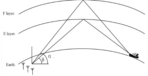
Consider a MIMO linear array radar withM transmitting elements andN receiving elements. In order to simplify the derivation, we assume that the transmitter and receiver are co-located with the same number of elements, i.e., M = N. Let X= [x₁,x2, . . . ,xM] be the group of M orthogonal signals to be transmitted, Xi ∈CK×1,i= 1, . . . , M,K be the number of transmitted signal samples. C indicates the complex number domain. The two-layer ionospheric model is composed of E layer and F layer [14], and the target is a far-field point target. According to Fig. 1, there are four modes of multipath propagation, i.e., E-E, E-F, F-E, F-F (e.g., E-F mode means that the probing signal is reflected by the E-layer, target and F-layer consecutively before reaching the receiver). For the receiving elements, there are two different DOAs (α andβ),Yα= [yα1,yα2, . . . ,yαN] andYβ = [y

β

1,y

β

2, . . . ,y

β

N] represent received

echoes from the angles of α and β respectively,yα_i,yβ_i ∈CK×1,i= 1,2, . . . , N. Θα = [θ1α,θα2, . . . ,θαN] and Θβ = [θ₁β,θβ2, . . . ,θ

β

N] represent the noise matrices from α and β respectively, θαi,θβi ∈ C

K×1

, i= 1,2. . . , N.

In detail,Yα consists of two components: one of them is obtained by transmitting a signal through the route formed by E-F mode. The other is obtained through the route formed by F-F mode. Similarly,

Yβ consists of two components: one of them is obtained by transmitting a signal through the route formed by F-E mode and the other is obtained through E-E mode.

(3)

Figure 1. MIMO-OTHR geometric model based on the two-layer ionospheric model.

as ν = [ν1, ν2, . . . , νN]T [12]. For DOA α and β, we have two receiving steering vectors as ν(α) = [ν1(α), ν2(α), . . . , νN(α)]T,ν(β) = [ν1(β), ν2(β), . . . , νN(β)]T, and ν =ν(α) +ν(β). For each yαi,

it consists of two components: the ﬁrst one denotes the signal reﬂected by the E-layer before reaching the target and can be expressed as

S1 =

M

i=1

δi1Eφ1iEμixi(t−τi1E) +θ1E, (1)

where δi1E is the E-layer reﬂecting response factor of the probing signal transmitted by the ith

transmitting element before reaching the target, φ1E

i the channel response factor of the probing

signal transmitted by the ith transmitting element before reaching the target, τi1E the time delay

of the probing signal transmitted by the ith transmitting element before reaching the target, θ1E =

θ11E, θ21E, . . . , θ1NE

T

the channel noise matrix before reaching the target.

S1 is then backscattered by the target as follows,

S2=

M

i=1

εiδ1iEφ1iEμixi(t−τi1E) +θ1E, (2)

whereεi is the backscattering coeﬃcient of sea clutter.

After being reﬂected by the F-layer and received by thejth receiving element, j= 1,2, . . . , N, we can obtain

S3 =

ε1δ11Eφ11Eμ1x1(t−τ11E −τ12F)νj(α)δ21Fφ21F+δ12Fφ12Fνj(α)θ1E+θ2F

+ε2δ21Eφ12Eμ2x2(t−τ21E−τ22F)νj(α)δ22Fφ22F+δ22Fφ22Fνj(α)θ1E +θ2F

+. . .+εMδ1MEφ1MEμMxM(t−τM1E −τM2F)νj(α)δ2MFφ2MF+δM2FφM2Fνj(α)θ1E+θ2F

=

M

i=1

εiδ1iEφ1iEδi2Fφ2iFνj(α)μi

hcomp_i,j 1

xi(t−τi1E−τi2F)

+νj(α)δ12Fφ21F +δ22Fφ22F +. . .+δM2Fφ2MF

θ1E₊_M_θ2F

θcompj 1

, (3)

where δi2F is the F-layer reﬂecting response factor of the probing signal transmitted by the ith

transmitting element after being scattered by the target,φ2F

i the channel response factor of the probing

signal transmitted by the ith transmitting element after being scattered by the target, τi2F the time

delay of the probing signal transmitted by the ith transmitting element after being scattered by the target, θ2F =θ12F, θ22F, . . . , θN2F

T

(4)

Notice that S3 only contributes one component for the echo yαi. Let S3=ycomp 1

j , hcompi,j 1 =

εiδ1iEφ1iEδ2iFφi2Fνj(α)μi,θjcomp1 =νj(α)δ21Fφ21F +δ22Fφ22F +. . .+δ2MFφ2MF

θ1E₊_M_θ2F _and _τcomp1

i =

τi1E +τi2F, we can get

ycomp_j 1 =

M

i=1

hcompi,j 1xi

t−τicomp1

+θcomp_j 1. (4)

Similarly, we can obtain the other component of the echo which is reﬂected by the F-layer, target, then F-layer at thejth receiving element,

ycomp_j 2 =

M

i=1

hcompi,j 2xi

t−τicomp2

+θcomp_j 2, (5)

The initial transmitted waveform is the linear frequency modulation continuous wave (LFMCW) which is usually utilized by traditional OTHRs,τicomp1,τicomp2 T, soxi(t−τicomp1) andxi(t−τicomp2)

can be approximated bye−j2πf0τicomp1_x_i₍_t_{) and}_e−j2πf0τicomp2_x_i₍_t_{) respectively.} _f₀_{is the carrier frequency}

and q the frequency modulation slope. The detailed derivation is given in Appendix A. The total received echo at thejth receiving element can be expressed as

yj =yjcomp1+ycompj 2= M

i=1

hcompi,j 1e−j2πf0τ

comp1

i ₊_hcomp2

i,j e−j2πf0τ

comp2

i

xi+

θcomp1

j +θjcomp2

. (6)

Lethi,j =hcompi,j 1e−j2πf0τ

comp1

i ₊_hcomp2

i,j e−j2πf0τ

comp2

i _,θj ₌θcomp1

j +θcompj 2, we get

yj = M

i=1

hi,jxi+θj. (7)

Since all the derivation above is for the echo coming from the DOAα, Eq. (7) can be rewritten as

y_jα=

M

i=1

hαi,jxi+θαj, (8)

where hαi,j ∈ C1×1,(i = 1,2, . . . , M, j = 1,2, . . . , N) represents the target response between the ith

transmitting element andjth receiving element if the DOA is α.

LetHα=

⎡ ⎢ ⎣

hα1,1 . . . hα1,N ..

. . .. ... hαM,1 . . . hαM,N

⎤ ⎥

⎦,Yα=[yα1,y2α, . . . ,yαN], Θα= [θ

α

1,θ2α, . . . ,θNα], we obtain

Yα=XHα+Θα. (9)

In a similar way, the echo from the DOAβ can be expressed as

Yβ=XHβ+Θβ, (10)

where Hβ =

⎡ ⎢ ⎣

hβ1,1 . . . h

β

1,N ..

. . .. ... hβ_M,₁ . . . hβ_M,N

⎤ ⎥

⎦, hβi,j ∈ C1×1, (i = 1,2, . . . , M, j = 1,2, . . . , N) represents the

target response between the ith transmitting element and jth receiving element if the DOA isβ. Since the ionosphere changes all the time, its movement and instability can cause the echo’s Doppler spectrum to shift and become more broad. Furthermore, when the OTHR probes a target on the sea, the impact of sea clutter can’t be signiﬁcant. Therefore, we improve the model under investigation by adding the following features:

(1) The backscattering coeﬃcient of sea clutter εi is generated by the high frequency (HF)

(5)

(2) Focus on slow moving target on the sea, and the product of the reﬂecting response factor δi

and channel response factorφi is generated by the K-distribution model [18].

(3) Hα,Hβ,Θα,Θβ are the product of several random variables. According to the central limit

theorem, when the samples are suﬃcient, Hα,Hβ,Θα,Θβ follow the multivariate normal distributions

with assumed zero means. Then we can easily ﬁnd that Eqs. (9) and (10) are Gaussian distributed with zero means and covariance matricesXR_HαXH+RΘα,XRHβXH+RΘβ.

Based on Eqs. (9) and (10), the following terms will be used in the next section:

R_Yα = E

YαYH_α=XR_HαXH+RΘα, (11)

R_Yβ = E

YβY_βH=XR_HβXH+RΘβ, (12)

R_Yα,Yβ = E

YαYHβ

=XR_Hα,HβXH+Rθα,θβ, (13)

R_Hα = E

HαHHα, (14)

R_Hβ = E

HβHHβ, (15)

R_Hα,Hβ = E

HαHHβ

, (16)

R_Θα = E

ΘαΘHα, (17)

R_Θ_β = EΘβΘHβ, (18)

R_Θα,Θβ = E

ΘαΘH_β . (19)

3. TWO-STEP WAVEFORM OPTIMIZATION ALGORITHM

This section introduces the two-step waveform optimization algorithm. The detection performance of MIMO-OTHR depends on the echo’s Doppler frequency and received signal-to-clutter ratio (SCR) but does not depend on speciﬁc waveforms. When considering the orthogonality of the transmitted waveforms and the inﬂuence of ionosphere to echoes, it is important to design optimized waveforms that are suitable for the multi-layer ionospheric propagation circumstance, which should also be able to reduce the impact of clutter, interference and noise.

Based on the groundwork from [15, 16, 19, 20], which applied mutual information theory to design of MIMO radar waveform in order to improve target detection performance, we propose a novel two-step waveform optimization algorithm (named Max-Min algorithm) for MIMO-OTHR.

The ﬁrst step of the algorithm is to maximize the mutual information between the echo (Yα or

Yβ) and target response matrix (Hα orHβ) at the same DOA (αorβ), in order to degrade the impact

of noise (Θα or Θβ). The second step is to minimize the mutual information between Yα and Yβ,

so as to make sure that the echoes from diﬀerent DOAs are uncorrelated and can suppress the strong clutter and interference by utilizing multi-path echoes. We introduce a feedback loop to enhance the algorithm, which adjusts the waveforms of the transmitter based on the receiver information, for time varying environment.

3.1. Step 1: Maximize Mutual Information Between the Echo and Target Response Matrix at the Same DOA

According to the classical deﬁnition of mutual information [15], we get

I(Y_α;Hα|X) = h(Yα|X)−h(Yα|H_α,X) =h(Yα|X)−h(Θα), (20)

I(Y_β;Hβ|X) = h(Yβ|X)−h

Yβ|Hβ,X

=h(Yβ|X)−h(Θβ), (21)

(6)

multi-dimensional random variables. According to the central limit theorem, Yα and Yβ follow the multivariate normal distribution. So we get

p(Yα|X) = exp

−trXR_HαXH+RΘα

₋1

YαY_αH

πNKdetN(XR_HαXH+RΘα)

, (22)

p(Yβ|X) =

exp

−trXR_H_βXH+R_Θ_β−1YβYβH

πNKdetNXR_H_βXH+R_Θ_β , (23)

where p(Yα|X) and p(Yβ|X) are the conditional probability density functions (PDF) of Yα and Yβ

given X. tr(·) is the trace of a matrix and det(·) the determinant of a matrix. The entropies of the received echoes Yα and Yβ are expressed as

h(Yα|X) =−

p(Yα|X) ln [p(Yα|X)]dYα=N Kln (π)+N K+NlndetXR_HαXH+RΘα

,(24)

h(Yβ|X) =−

p(Yβ|X) ln [p(Yβ|X)]dYβ=N Kln (π)+N K+NlndetXRHβXH+RΘβ

. (25)

In a similar way, we obtain the entropies of the noise matrices Θα andΘβ as

h(Θα) = −

p(Θα) ln [p(Θα)]dΘα =N Kln (π) +N K+Nln [det (RΘα)], (26)

h(Θβ) = −

p(Θβ) ln [p(Θβ)]dΘβ =N Kln (π) +N K+NlndetRΘβ

. (27)

Using (24)–(27) to solve (20) and (21), we have

I(Y_α;H_α|X) = NlndetXR_HαXH+RΘα

−Nln [det (R_Θα)], (28)

I(Y_β;H_β|X) = NlndetXR_H_βXH+R_Θ_β−NlndetR_Θ_β. (29) Maximizing I(Y_α;H_α|X) in Eq. (28) orI(Y_β;H_β|X) in Eq. (29) under the condition of the same total transmission power budgetP0 yields a set of optimal waveforms ensembles Sx.

3.2. Step 2: Minimize Mutual Information between the Echoes from Diﬀerent DOAs

Refer to [20], the joint entropy of (Yα,Yβ) can be derived as

h(Yα,Yβ|X) = −

p(Yα,Yβ|X) lnpYα,Y_β|XdYαdYβ

= 2N Kln (π) + 2N K+NlndetXR_HαXH+RΘα

+NlndetXR_H_βXH+R_Θ_β+Nln

det

IM×M −[Dα,β]2

, (30)

where IM×M is the identity matrix with dimension M ×M; Dα,β =

⎡

⎣ d1 _{. . .}

dM

⎤

⎦ is the diagonal

matrix obtained by the singular value decomposition (SVD) of the covariance matrix R_Yα,Yβ; the

diagonal elementsd1≥d2 ≥. . .≥dM. YαandYβare the whitening matrix ofYαandYβ, respectively,

and

R_Y_α_,_Y_β=E

YαYβH

=

R−1_Y_αR_Yα,Yβ

R−1_Y_β

H

. (31)

According to Eqs. (24), (25) and (30), the mutual information betweenYα andYβ can be derived as

I(Yα,Yβ) = h(Yα|X) +h(Yβ|X)−h(Yα,Yβ|X)

= −Nln

det

IM_×M −[Dα,β]2

=−N

M

m=1

ln1−d2m

(7)

We can thus minimize Eq. (32) with the constraint of total overall transmission power P0 to ﬁnd the optimal waveformX from the set of optimal waveform ensembles S_x.

3.3. Algorithm Implementation

By employing the MVDR adaptive beam-former for transmitting and receiving and based on the array signal processing theory, the proposed Max-Min algorithm is summarized as follows:

(1) At timet, use the MVDR adaptive beam-former to process the received echoes and obtain Yα and

Yβ. At the initial time t= 0, LFMCW is transmitted.

(2) Maximize Eq. (28) or (29) under the constraint of total transmission power P0 to ﬁnd a set of optimal waveforms ensemblesS_x.

Taking Eq. (28) as an example, we have

max

Sx Nln

detXR_HαXH+RΘα

−Nln [det (R_Θα)]

s.t. trXXH≤P0 .

(33)

For Eq. (29), similarly,

max

Sx Nln

detXR_H_βXH+R_Θ_β−NlndetR_Θ_β

s.t. trXXH≤P0 .

(34)

The choice of Eq. (33) or (34) depends on the practical scenario: if the SCR is low, maximize (34) as the E-layer is more stable than F-layer; otherwise, Eq. (33) will be selected.

(3) Minimize Eq. (32) under the constraint of total transmission powerP0to ﬁnd the optimal waveform

Xfrom S_x. This step is simpliﬁed as

min

X

−N

M

m=1

ln1−d2m

s.t. trXHX≤P0,

(35)

where R_Hα, RHβ, RΘα and RΘβ can be obtained by using Eqs. (14), (15), (17), (18). At the initial

timet= 0,R_H_α_|_t₌₀,R_H_β_|_t₌₀,R_Θ_α_|_t₌₀ and R_Θ_β_|_t₌₀ can be obtained by ionosphere detection devices. (4) At the timet+ 1, transmit the optimal waveform Xobtained at the time t.

(5) Repeat step (1)–(4) iteratively.

4. SIMULATION RESULTS

In this section, numerical experiments are conducted to evaluate performance of the waveforms obtained by the proposed algorithm. We choose the E-layer and F-layer with height of 100 km and 220 km respectively. Each propagation channel is generated following the Watterson model [17], and the clutter model is based on K-distribution [18] with the shape parameter ν = 1. The initial waveform of each antenna element is LFMCW. We set the repetition time as 0.25 s, the bandwidth as 20 kHz and the carrier frequency as 3 MHz. A point target on the sea surface is set to be about 1000 km away from the radar, with a velocity of 15 m/s. The co-located receiving and transmitting antenna array have the same number of elements, i.e., M = N, and are arranged as minimum redundancy linear array. The reason to choose the minimum redundancy linear array scheme is that its main lobe is narrower than the uniform linear array schemes with the same number of elements. Such narrow main lobe is particularly eﬀective for MIMO-OTHR to distinguish and identify the multipath echoes that come at very similar angles. The clutter-to-noise ratio (CNR) and received signal-to-clutter ratio (SCR) are calculated by CNR (dB) =10 log₁₀

Pclutter

Pnoise

and SCR (dB) =10 log₁₀

_P

signal

Pclutter

, where Psignal is the

(8)

(a) (b)

(c) (d)

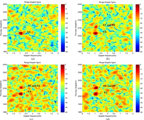
Figure 2. Range-Doppler maps for diﬀerent iteration numbers of the Max-Min algorithm (a) t = 0, (b)t= 10, (c)t= 20, and (d) t= 50 for M = 12, CNR = 20 dB, SCR = 10 dB.

The ﬁrst experiment investigates the range-Doppler improvement with diﬀerent SCR condition when the clutter is strong (CNR = 20 dB), and the results are shown in Fig. 2 and Fig. 3. The 12 array elements are arranged as minimum redundancy linear array with unit spacing{1,2,3,7,7,7,7,7,4,4,1}, spanning 50 units where a unit is half a wavelength [21].

Figures 2(a)–2(d) are the range-Doppler maps of the echoes with diﬀerent time length (denoted by the number of iterations), with other parameters M = 12, CNR = 20 dB, SCR = 10 dB. The vertical-axis represents the total transmission range from transmitter to receiver (two-way range), the horizontal-axis represents the Doppler frequency and the colorbar represents normalized intensity (dB) of the echo strength. Without proper processing, echoes of E-F and F-E modes overlap on the range-Doppler map because they have the same transmission range and similar channel response. In Fig. 2(a), only the echo of E-E mode is clearly shown on the map at the initial time. In Figs. 2(b)–2(d), as the algorithm iterations increases, echoes of E-F and F-E modes gradually appear on the range-Doppler map, but the signal of F-F mode is still overwhelmed by clutter and noise.

(9)

(a) (b)

(c) (d)

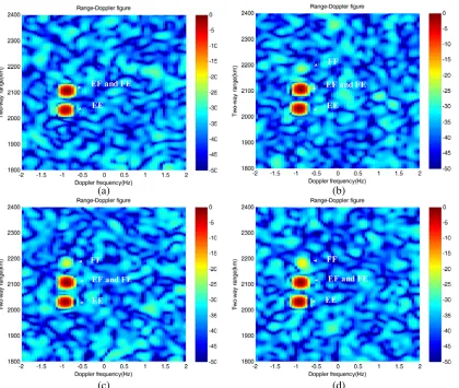
Figure 3. Range-Doppler maps for diﬀerent iteration numbers of the Max-Min algorithm (a) t = 0, (b)t= 10, (c)t= 20, and (d) t= 50 for M = 12, CNR = 20 dB, SCR = 15 dB.

algorithm iterations increases, the echo of F-F mode gradually appears on the map. Because this mode is not interfered by other propagations, it can better exhibit the target characteristics and has superior detection performance. Furthermore, the target location is more precise and the range resolution has been improved based on the geometric model shown in Fig. 1 given the ionospheric heights.

The next group of experiments investigate the range resolution performance of the proposed algorithm and the condition of diﬀerent CNRs. Fig. 4 and Fig. 5 show the results.

Figure 4 gives the range resolution curve when M = 12, CNR = 20 dB, and SCR = 15 dB. The vertical-axis represents the range resolutions (km) and the horizontal-axis represents the number of iterations. The range resolution is about 30 km before the application of the Max-Min algorithm. The Maximization step (Step 1) does not result significant range resolution improvements, because this step only focuses on noise suppression, and CNR = 20 dB means that the ionosphere and sea clutter are much stronger than noise. Under this condition, the application of the Minimization algorithm may provide more benefits (about 9 km improvement of range resolution after 60 iterations) since it focuses on minimizing correlation of the echoes from different DOAs and suppressing clutter and interference by utilizing two different propagation echoes.

(10)

Max-5 10 15 20 25 30 35 40 45 50 55 60 18 20 22 24 26 28 30 32 Iteration Range r e s o lu ti o n (k m ) Max-Min optimization Min optimization only Max optimization only Non-optimization

Figure 4. Range resolution optimization for M = 12, CNR = 20 dB, SCR = 15 dB.

5 10 15 20 25 30 35 40 45 50 55 60 18 20 22 24 26 28 30 32 Iteration Range r e s o lu ti o n (k m ) Max-Min optimization Min optimization only Max optimization only Non-optimization

Figure 5. Range resolution optimization for M = 12, CNR = 0 dB, SCR = 15 dB.

-10 -5 0 5 10 15 20

0 0.1 0.2 0.3 0.4 0.5 0.6 0.7 0.8 0.9 1 SCR(dB) P d (P robabi li ty o f d e te c ti o n ) a1 a2 b1 b2 c1 c2 d1 d2 e1 e2 f1 f2 g

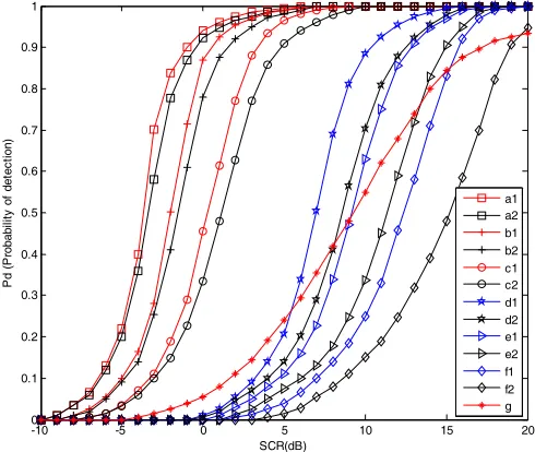
Figure 6. Probability of detection versus SCR: a1: optimized curve for M = 12 and CNR = 0 dB (square solid line), a2: non-optimized curve for M = 12 and CNR = 0 dB (square dotted line), b1: optimized curve for M = 8 and CNR = 0 dB (plus solid line), b2: non-optimized curve for M = 8 and CNR = 0 dB (plus dotted line), c1: optimized curve for M = 4 and CNR = 0 dB (circle solid line), c2: non-optimized curve for M = 4 and CNR = 0 dB (circle dotted line), d1: optimized curve for M = 12 and CNR = 20 dB (pentacle solid line), d2: non-optimized curve for M = 12 and CNR = 20 dB (pentacle dotted line), e1: optimized curve for M = 8 and CNR = 20 dB (triangle solid line), e2: non-optimized curve for M = 8 and CNR = 20 dB (triangle dotted line), f1: non-optimized curve for M = 4 and CNR = 20 dB (diamond solid line), f2: non-optimized curve for M = 4 and CNR = 20 dB (diamond dotted line), g: SISO curve for M = 1 and CNR = 0 dB (asterisk solid line).

Min algorithm has the best performance and achieves a 9 km improvement of range resolution after 60 iterations.

(11)

The false alarm probability is set to 10−4. Fig. 6 compares the performance of 6 groups of experiment results (a1, a2; b1, b2; c1, c2; d1, d2; e1, e2; f1, f2), each denoting a diﬀerent set of the number of antennas and CNRs condition. We can have the following observations from Fig. 6:

(1) Detection probability is signiﬁcantly improved after the application of the proposed algorithm when SCR is constant.

(2) Detection probability of the proposed algorithm increases when the number of antennas grows, if other conditions are constant.

(3) Detection probability of the proposed algorithm increases when CNR rises, if other conditions are constant.

Practical OTHR may receive much stronger clutter and interference than noise, i.e., CNR can be as high as 20–40 dB (or 40–60 dB if Bragg scatter and transient interference are included). The proposed Max-Min optimization algorithm is directly targeting this over-the-horizon circumstance, and is thus particularly useful in OTHRs.

Another interesting scenario is obtained whenM = 1 and CNR = 0 dB, which means that there is only one antenna element and thus a single-input and single-output (SISO) system is under investigation. As shown in Fig. 6, its performance is obviously worse than MIMO-OTHR.

5. CONCLUSION

This paper considers a multi-layer ionospheric model for OTHR radars and suggests the application of MIMO radar technique to enhance the detection performance of such type of radars. A two-step waveform optimization algorithm called Max-Min algorithm is proposed, where the first step is to maximize the mutual information between the echo and transmission response from the same DOA, and the second step is to minimize the mutual information between echoes from different DOAs. Simulation results verify that the proposed algorithm can improve the performance of MIMO-OTHR in terms of the detection probability and range-Doppler resolution. Simulation results further indicate that when CNR approaches −∞, the performance of MIMO-OTHRs becomes similar to horizon MIMO radars, since the Max algorithm (Step 1) plays a major role in waveform optimization; when CNR increases, the Min algorithm (Step 2) contributes more in the waveform optimization. However, the two-layer ionospheric model is still a very simplified representation of the real world. More accurate models can better characterize the ionosphere.

APPENDIX A. TIME DELAY APPROXIMATION OF LFMCW

The initial LFMCW of ith transmitting element can be expressed as

xi(t) =a0ej2πf0t

M−1

m=0

p(t−mT),

p(t) =

ejπqt2 0≤t < T

0 others .

(A1)

where a0 is the signal amplitude, f0 the carrier frequency, q the frequency modulation slope, T the repetition time, and M the number of the pulses in each repetition time. The time delay τicomp1, τicomp2 T, thus

xi

t−τicomp1

=a0ej2πf0(t−τ

comp1

i )

M−1

m=0 p

t−τicomp1−mT

≈a0ej2πf0te−j2πf0τ

comp1

i

M−1

m=0

p(t−mT) =e−j2πf0τicomp1_xi₍_t₎

(A2)

In a similar way, we can obtain

xi(t−τicomp2)≈e−j2πf0τ

comp2

(12)

REFERENCES

1. Skolnik, M. L., Radar Handbook, 3rd edition, 807–876, New York, McGraw-Hill, 2008.

2. Headrick, J. M. and J. F. Thomason, “Applications of high frequency radar,”Radio Science, 1045– 1054, 1998.

3. Howland, P. E. and D. C. Copper, “Use of the Wigner-Ville distribution to compensate for ionospheric layer movement in high-frequency sky-wave radar system,” Radar and Signal Processing, IEE Proceedings F, Vol. 140, No. 1, 29–36, Feb. 1993.

4. Olkin, J. A., W. C. Nowlin, and J. R. Bamum, “Detection of ships using OTH radar with short integration times,” Proceedings of the 1997 IEEE National Radar Conference, 1–6, May 1997. 5. Krolik, J., V. Mecca, O. Kazanci, and I. Bilik, “Multipath spread-Doppler clutter mitigation for

over-the-horizon radar,”Proceedings of the 2008 IEEE Radar Conference, 1–5, 2008.

6. Ravan, M., R. S. Adve, and R. J. Riddolls, “MIMO fast fully adaptive processing in Over-the-Horizon radar,” Proceedings of the 2011 IEEE Radar Conference, 538–542, May 2011.

7. Frazer, G. J., Y. I. Abramovich, and B. A. Johnson, “Multiple-input multiple-output over-thehorizon radar: Experimental results,”IET Radar, Sonar & Navigation, 290–303, Aug. 2009. 8. Frazer, G. J., Y. I. Abramovich, and B. A. Johnson, “HF skywave MIMO radar: The HILOW

experimental program,” Proceedings of the 42nd Asilomar Conference on Signals, Systems and Computers, 639–643, Oct. 2008.

9. Riddolls, R. J., M. Ravan, and R. S. Adve, “Canadian HF over-the-Horizon Radar experiments using MIMO techniques to control auroral clutter,” Proceedings of the 2010 IEEE Radar Conference, 718–723, May 2010.

10. Olkin, J. A., W. C. Nowlin, and J. Barnum, “Detection of ships using OTH radar with short integration times,” Proc. IEEE Nat. Radar Conf., 1–6, Syracuse, NY, May 1997.

11. Abramovich, Y. I., G. J. Frazer, and B. A. Johnson, “Iterative adaptive Kronecker MIMO radar beamformer: Description and convergence analysis,” IEEE Transactions on Signal Processing, Vol. 58, No. 7, 3681–3691, Mar. 2010.

12. Abramovich, Y. I., G. J. Frazer, and B. A. Johnson, “Principles of mode-selective MIMO OTHR,”

IEEE Transactions on Aerospace and Electronic Systems, Vol. 49, No. 3, 1839–1868, Jul. 2013. 13. Luo, Y. and Z. Zhao, “Trajectory optimisation method by using independent component analysis

for MIMO-OTHR target tracking,” Electronics Letters, Vol. 51, No. 13, 1020–1021, 2015.

14. Pulford, G. W. and R. J. Evans, “A multipath data association tracker for over-the-horizon radar,”

IEEE Transactions on Aerospace and Electronic Systems, Vol. 34, No. 4, 1165–1183, Oct. 1998. 15. Yang, Y. and R. S. Blum, “MIMO radar waveform design based on mutual information and

minimum mean-square error estimation,”IEEE Transactions on Aerospace and Electronic Systems, Vol. 43, No. 1, 330–343, Jan. 2007.

16. Tang, B., J. Tang, and Y. Peng, “MIMO radar waveform design in colored noise based on information theory,”IEEE Transactions on Signal Processing, Vol. 58, No. 9, 4684–4697, Sep. 2010. 17. Perl, J. M. and D. Kagan, “Real-time HF channel parameter estimation,” IEEE Transactions on

Communications, Vol. 34, No. 1, 54–58, Jan. 1986.

18. Watts, S., “Modeling and simulation of coherent sea clutter,” IEEE Transactions on Aerospace and Electronic Systems, Vol. 48, No. 4, 3303–3317, Oct. 2012.

19. Sen, S. and A. Nehorai, “OFDM MIMO radar with mutual-information waveform design for low-grazing angle tracking,” IEEE Transactions on Signal Processing, Vol. 58, No. 6, 3152–3162, Mar. 2010.

20. Chen, Y., Y. Nijsure, C. Yuen, Y. H. Chew, Z. Ding, and S. Boussakta, “Adaptive distributed MIMO radar waveform optimization based on mutual information,” IEEE Transactions on Aerospace and Electronic Systems, Vol. 49, No. 2, 1374–1385, Apr. 2013.