3-D Imaging of High-Speed Moving Space Target via Joint
Parametric Sparse Representation
Yuxue Sun1, *, Meng Jiang5, Ying Luo1, 2, 3, Qun Zhang1, 2, 4, and Chunhui Chen1
Abstract—The high-speed moving of space targets introduces distortion and migration to range profile, which will have a negative effect on three-dimensional (3-D) imaging of targets. In this paper, based on joint parametric sparse representation, a 3-D imaging method for high-speed moving space target is proposed. First, the impact of high speed on range profile of target is analyzed. Then, based on an L-shaped three-antenna interferometric system, a dynamic joint parametric sparse representation model of echoes from three antennas is established. The dictionary matrix is refined by iterative estimation of velocity. Moreover, an improved orthogonal matching pursuit (OMP) algorithm is proposed to recover interferometric phase information. Finally, with the phase information, interferometric processing is conducted to obtain the 3-D image of target scatterers. The simulation results verify the effectiveness of the proposed method.
1. INTRODUCTION
With the increasing number of space targets, such as space debris, satellites, and ballistic missiles, the space environment is becoming more and more complex. Thus it is of great significance to conduct tracking, measuring, categorization and recognition of space targets to ensure space security and stimulate the development of space technology.
Three-dimensional (3-D) imaging technique is capable of providing abundant features of target outline, size, micro-motional parameters, etc. Thus the 3-D imaging technique for space targets has been a hot researching spot in radar imaging field [1]. The existing 3-D imaging methods of space targets mainly include monostatic-radar-based imaging methods [2, 3] and multistatic-radar-based imaging methods [4, 5]. Moreover, a novel interferometric 3-D imaging method of space target based on an L-shaped three-antenna configuration has been proposed in the authors’ previous work [6]. On the condition of multiple antennas, only micro-motional characteristic in the radial direction of radar can be extracted from the echo of each antenna. In addition, the extracted micro-motional characteristics from all antennas are approximately the same, since there is not much difference between their observation angles. However, the different locations of antennas produce delicate differences among the ranges from target to each antenna, which will introduce corresponding phase difference (i.e., interferometric phase) among the received echoes of each antenna. The interferometric phase in reverse reflects the position of target. Ref. [6] makes use of different micro-motional characteristics of multiple target scatterers to separate the echo of each scatterer on range-slow-time plane. Then interferometric processing is conducted to obtain interferometric phase, and a 3-D image of target is thus reconstructed through a geometrical transform between the interferometric phase and target position. Compared with
Received 14 April 2017, Accepted 24 June 2017, Scheduled 10 July 2017 * Corresponding author: Yuxue Sun ([email protected]).
monostatic-radar-based imaging method, the interferometric imaging method provides a real target 3-D size for more reliable target recognition; meanwhile, it avoids complex synchronization and joint processing of echoes from different radars compared with multistatic-radar-based imaging methods. Besides, the interferometric imaging method of space target realizes a time-varying imaging during radar irradiation time with obtaining an illustration of target motion trajectory, thus providing a new direction for 3-D imaging and characteristic extraction of space target.
However, space target is usually with a high-speed moving velocity, which will introduce distortion and migration to range profile [7]. Interferometric 3-D imaging is conducted on range-slow-time plane, thereby the distortion and migration of range profile will bring many adverse effects to 3-D imaging, which mainly include: (i) the distortion of range profile will affect the extraction of trajectory on range-slow-time profile, resulting in difficulty of separating echoes of multiple target scatterers; (ii) interferometric phase is hard to be extracted from distorted range profile; (iii) impulse migration changes the phase of target echo thus resulting in reconstructed target position obtained by interferometric processing deviating from real value; (iv) the migration of range profile affects the range position reconstruction of target scatterer, since the range position is directly obtained by range-slow-time profile. Thus, compensating for distortion and migration of range profile is an important step in the procedure of 3-D interferometric imaging of space targets.
This paper introduces parametric sparse representation into interferometric 3-D imaging of space targets with high-speed motion. According to the characteristic of target echo, a sensing matrix is first constructed, which contains unknown motion velocity of the target. And a joint sparse representation model of the echoes from three antennas is accordingly set up. Then, the optimal velocity is obtained by iteratively refining the estimated velocity and sensing matrix. Based on the estimated optimal velocity, an improved orthogonal matching pursuit (OMP) algorithm is adopted to obtain the range position of target and phase information on range-slow-time profile. Finally, via interferometric processing on the obtained phase information, the 3-D image of target is reconstructed. Simulation results verify that the proposed method is capable of compensating the effect of high-speed motion while preserving the interferometric phase for 3-D imaging of space targets.
2. SIGNAL MODEL
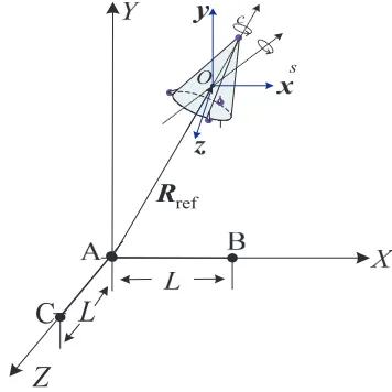
The interferometric 3-D imaging system adopts three L-shaped antennas as shown in Fig. 1. Orthogonal antennasA,Band antennasA,Care composed of interferometric antenna pairs onXOY plane andYOZ plane, respectively. The length of antenna baseline isL. Radar coordinateXYZ is originated at antenna
A, and target coordinate xyz is originated at a pointOon the target. The axes of target coordinate are parallel with those of radar coordinate, respectively. Antenna A transmits linear frequency modulated (LFM) signal. The received signal of antenna Ais
sA
ˆ
t, tm
=
K
k=1
σkrect
ˆt
−2rAk(ˆt, tm)/c
Tp
·exp
j 2πfc
ˆ
t−2rAk(ˆt, tm)
c
+jπμ
ˆ
t−2rAk(ˆt, tm)
c
2
(1)
where
rect
ˆt
Tp
= 1, −Tp/2≤ˆt≤Tp/2
0, others (2)
In Eq. (1), rAk(ˆt, tm) is the range from the kth scatterer to antenna A, c the wave velocity, fc the carrier frequency, Tp the pulse width, μ the modulation rate, ˆt = t−tm the fast time, tm = mT,
m = 0,1,2, . . . , M −1 the slow time, M the pulse number, T the pulse repetition duration, and σk
the scattering coefficient of the kth scatterer. The range from point O to antenna A is chosen as the reference range, which is Rref(tm) = RAO(tm). Since the target moves with a high speed, it yields
rAk(ˆt, tm) = rAk(tm) +vrtˆ, where rAk(tm) is the range from the kth scatterer to antenna A at each
slow-time sampling point, and vr is the radial velocity relative to radar. After “dechirp”, Eq. (1)
becomes
sAdt, tˆ m=
K
k=1
σ
Akrect
ˆt
−2rAk(ˆt, tm)/c
Tp
·expjφ1+φ2ˆt+φ3tˆ2
where
σAk = σk·exp
−j4π
c fcRΔAk(tm)
(4)
φ1(tm) =
4πμ
c2
r2
Ak(tm)−R2ref(tm)
φ2(tm) = −
4π
c μRΔAk(tm)−
4π
c fcvr+
8πμ
c2 rAk(tm)vr (5)
φ3 = −
4π
c μvr+
4πμ
c2 v
2
r
and RΔAk(tm) = rAk(tm) − Rref(tm). σAk is the range profile of the kth scatterer obtained by
antennaA, of which the phase term is the essence of interferometric imaging. Since there is almost no difference between view angles of all antennas, the amplitudes of range profiles of them should remain a constant [8, 9]. Thus the range profiles of antenna B and antenna C can be represented as
σBk = σk·exp
−j2π
c fc(RΔAk(tm) +RΔBk(tm))
(6)
σ
Ck = σk·exp
−j2π
c fc(RΔAk(tm) +RΔCk(tm))
(7)
where RΔBk(tm) =rBk(tm)−Rref(tm) and RΔCk(tm) = rCk(tm)−Rref(tm). rBk(tm) and rCk(tm) are
range from the kth scatterer to antenna B and C, respectively. φ1 is relatively small and generally
can be ignored. In φ2, the first term −4πμRΔAk(tm)/c is the initial range position of scatterer and
the next two terms will introduce range migration. φ3 will introduce distortion to range profile. The
migration and distortion of range profile will both affect the interferometric 3-D imaging in the later processing, thus they must be compensated before conducting interferometric processing. It can be seen from Eq. (5) that the migration and distortion terms are both decided by velocity of target, thus estimating and compensating the velocity is the essence of eliminating migration and distortion of range profile.
O s
c
ref R
Z
C
L
Figure 1. Geometry of 3-D imaging system and space target.
3. PARAMETRIC SPARSE REPRESENTATION BASED 3-D IMAGING OF HIGH-SPEED SPACE MOVING TARGET
3.1. The Model of Joint Parametric Sparse Representation
which can be represented as
RΔ= [rΔ1, . . . , rΔi, . . . , rΔN] i= 1, . . . , N (8)
whererΔi =ri−Rref andri is the range from theith range bin to radar. During the imaging time, the
mth pulse received by antenna A is
sAdmˆt=
K
k=1
σAmk ϕ (9)
where
ϕ= rect
ˆt
−2rAk/c
Tp
·expjφ1+φ2ˆt+φ3ˆt2
(10)
Andϕrepresents the kernel function. After being discretized, Eq. (9) can be rewritten as
sAdm=Φ(vr)σAm+Em (11) where
Φ(vr) = [ϕ1, . . . ,ϕi, . . . ,ϕN] (12)
ϕi =
⎡ ⎢ ⎢ ⎢ ⎢ ⎢ ⎢ ⎣
exp(j (φ1(rΔi) +φ2(rΔi) ˆt1+φ3(rΔi) ˆt21))
.. .
exp(j (φ1(rΔi) +φ2(rΔi) ˆtj+φ3(rΔi) ˆt2j))
.. .
exp(j (φ1(rΔi) +φ2(rΔi) ˆtN +φ3(rΔi) ˆt2N))
⎤ ⎥ ⎥ ⎥ ⎥ ⎥ ⎥ ⎦ (13) ⎧ ⎪ ⎪ ⎪ ⎪ ⎪ ⎪ ⎨ ⎪ ⎪ ⎪ ⎪ ⎪ ⎪ ⎩
φ1(rΔi) =
4πμrΔi
c2 (rΔi+ 2Rref)
φ2(rΔi) =−
4π
c
vr
fc−2μ(rΔi+Rref)
c
+μrΔi
φ3(rΔi) =−
4π
c
μvr−μvr2
c
(14)
σ
Am =
σAm1exp
−j4π
c fcrΔ1
, . . . , σAmiexp
−j4π
c fcrΔi
, . . . , σAmNexp
−j4π
c fcrΔN
T
(15)
σAmi is the scattering coefficient of the ith range bin in interested area, T = [ˆt1, . . . ,tˆj, . . . ,ˆtN] the
sampling time sequence, N the number of sampling data, and Em the noise vector.
Through solving Eq. (11), the range profile σAm can be obtained. The sensing matrix Φ(vr)
is indeterminate since the velocity is unknown. Different velocities correspond to different sensing matrixes. Thus vr should be estimated at first. With a well estimated vr, the sensing matrix will match with echo signal. Thereby a focused range profile could be obtained. In this paper, an iterative optimization algorithm is applied to estimatevr. The velocity and sensing matrix are updated iteratively until the optimal solution is obtained. Then the range profile σAm can be solved by the following optimizing model:
minσAm0 s.t. sAdm−Φ(vr)σAm2≤ε (16) whereεis noise level.
In an interferometric imaging system, the phase information of echo should be as accurate as possible to ensure the imaging precision [10]. Thus a joint sparse representation model is established for ensuring the coherence of the reconstructed phase information from three antennas. Eq. (16) can be rewritten as
minσm2,1 s.t. sm−Φ(vr)σm2 ≤ε (17)
where σm2,1 =
|σ
Am|2+|σBm|2+|σCm|2 is mixed norm, sm = [sAdmsBdmsCdm] and σm =
3.2. 3-D Imaging Based on Improved Orthogonal Matching Pursuit Algorithm
The amplitudes of range profiles from the three antennas keep consistent, as mentioned before, thus the joint range profiles can be represented as
σ
m=Amp·ψ (18)
where Amp = diag(σ), σ = [σAm1, . . . , σAmi, . . . , σAmN] and ψ=[exp(jψA),exp(jψB),exp(jψC)]
is the phase vector of RΔ. ψA = [ψA1, . . . ψAi, . . . ψAN]T, ψB = [ψB1, . . . ψBi, . . . ψBN]T, ψC =
[ψC1, . . . ψCi, . . . ψCN]T. An improved OMP algorithm is developed to solve Eq. (17). The detail is
as follows:
Step 1 Initializing: The residual is r0 = sm. Iterative times are n = 1 and p = 1. The position
vector is Pos=∅. Matching vector set isAt=∅. Sparseness is Sp, and initial velocity is vrn.
Step 2 Seek for the matching vector and position: Search for the position of max (|ΦHn(vrn)r0|) and
denote its row number and column number as row and col, respectively. Update Pos = [Pos, row], At= [At, ϕrow].
Step 3 Estimate the amplitude:
amp=AtHAt−1AtHscol (19)
wherescol is thecolth column ofsm. Denote Val= diag(amp).
Step 4 Estimate the phase:
pha=ValH·AtHAt·Val−1ValH·AtH·scol (20) Step 5 Update the residual:
r0 =sm−At·Val·pha (21)
Step 6 Iterate to get the solution: p=p+ 1 and Φn(ϕrow) =0. RepeatStep 2 to Step 5 until p=Sp.
Step 7 Estimate the velocity: n=n+ 1 and set the termination thresholdη. Construct σm(n−1) by obtained amp and pha, then expand the sensing matrix using Taylor series expansion, that is
Φn−1
vr(n−1)≈Φn−1
vr(n−1)+ ∂Φn−1(vr)
∂vr
vr=vr(n−1)
·Δvr (22)
where Δvr is the increment of velocity. Substitute Eq. (22) into the object function vr = arg minsm−Φn−1(vr(n−1))·σm(n−1)2, then it yields minΔvrsm−Φn−1(vr(n−1))·σm(n−1)−Tn−1
Δvr2, where
Tn−1 =
∂Φn−1(vr)
∂vr
vr=vr(n−1)
·σm(n−1) (23)
Obtain the solution as
Δvr=
THT−1TH
sm−Φn−1
vr(n−1)·σ
m(n−1)
(24)
The velocity is computed asvrn =vr(n−1)+ Δvr. Substitute the newvrninto (22) and repeat the above
processing until |Δvr| ≤η.
Step 8 Obtain the range profile: construct Φn(vrn) using vrn and repeat Step 2 to Step 6. A
focused range profile is finally obtained.
The obtained position vector Pos contains the positions of scatterers in the range direction. Correspond these positions toRΔand thus they-axis positions of scatterers are obtained. phacontains
the phase information for interferometric processing andpha= [phaA,phaB,phaC]T, where phaA, phaB and phaC are the phases of range profiles from antenna A, B and C, respectively. Use the phase information, combining with Eqs. (4), (6) and (7), to conduct interferometric processing. The interferometric phases are
ψABk = angle(phaA∗k·phaBk) = 2π(RΔAk−RΔBk)/λ (25)
where “∗” represents conjugating operation; phaAk, phaBk and phaCk are the kth elements in corresponding phase vectors; λ is wave length. According to the geometrical relationship in Fig. 1, it yields
RΔAk−RΔBk= (rAk−Rref)−(rBk−Rref) =
2L(Xc+xk)−L2
rAk+rBk (27)
In far field, it yieldsrAk+rBk≈rAk+rCk≈2×(yk+Yc), whereykis the reconstructedy-axis position of the kth scatterer. Thus, reconstructed x-axis and z-axis position of the kth scatterer are
xk = ψABλ·(yk+Yc)
2πL +
L
2 −Xc (28)
zk = ψACλ·(yk+Yc)
2πL +
L
2 −Zc (29)
On the basis of the reconstructed 3-D positions [xk, yk, zk], k= 1,2, . . . , K of target scatterers, the 3-D image is thus obtained. During imaging time, repeat the 3-D imaging processing for each echo pulse, time-varying 3-D images are reconstructed.
4. SIMULATIONS AND ANALYSIS 4.1. Simulation Results
The antenna configuration in Fig. 1 is adopted. Suppose that the carrier frequency of transmitted signal is 20 GHz, bandwidth 750 MHz, pulse width 200µs, pulse repetition frequency 800 Hz, imaging time 1 s, range resolution 0.2 m and length of antenna baseline L = 100 m. The velocity of target is (4000, 0, 4000) m/s, and the radial velocity is vr = 5656.9 m/s. The target center is at (0, 500, 0) km at initial
time. Suppose that there are three scatterers. Considering the complex micro-motion of space targets, rotation and precession are simulated here. One of the three scatterers is rotating with rotation velocity
ωc= (5.45,0,30.94) rad/s. The other two are undergoing precessional motion, which contains the same
rotation with the first scatter and coning of velocityωs = (0,0,18.85) rad/s. The rotation period is 0.2 s
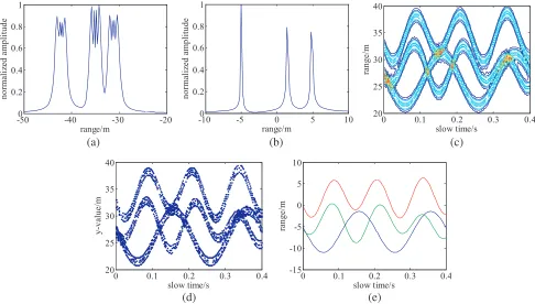
and the coning period is the 0.33 s. Under Nyquist sampling, range profile at each time slice will be affected by high speed motion. For an instance, the range profile at tm = 0.6 s is shown in Fig. 2(a). Fig. 2(b) shows the range profile when the velocity of target is 0 m/s attm = 0.6 s. It can be seen that range profile under high speed is seriously migrated and distorted. The range-slow-time profile is shown in Fig. 2(c). To better illustrate the figures, time span [0, 0.4 s] in figures is taken out. The migrated and distorted range-slow-time profile will affect both the abstracting the y-axis position of scatterer and interferometric phase. Fig. 2(d) shows y-axis positions abstracted by range-slow-time profile in Fig. 2(c). Fig. 2(e) shows the theoretical y-axis positions. As shown, abstracted y-axis positions are also migrated and distorted with many redundant points.
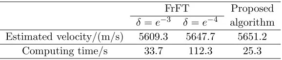
The initial velocity of target is set as 5500 m/s, and the estimated velocity is 5651.2 m/s. The compressing ratio is 0.8. In order to illustrate the performance of the velocity estimation in the proposed method, Fractional Fourier transform (FrFT) based velocity estimation algorithm in [11] is compared with the proposed algorithm. The FrFT based velocity estimation algorithm makes use of a priori information that the echo of high-speed moving target is multicomponent chirp signal and searches for the optimal order p to obtain velocity. While choosing different order-searching accuracy classes δ, different velocity accuracies are obtained. Table 1 shows the simulation results of the proposed algorithm and FrFT based algorithm with different order-searching accuracy classes. Each result is a mean of 50
Table 1. Comparison of two velocity-estimated algorithms.
FrFT Proposed
δ=e−3 δ =e−4 algorithm Estimated velocity/(m/s) 5609.3 5647.7 5651.2
-500 -40 -30 -20 0.2 0.4 0.6 0.8 1 range/m n o rm aliz ed a m p lit ud e
-100 -5 0 5 10
0.2 0.4 0.6 0.8 1 range/m n o rm aliz ed a m p lit ud e slow time/s ran g e/ m
0 0.1 0.2 0.3 0.4
20 25 30 35 40
0 0.1 0.2 0.3 0.4
20 25 30 35 40 slow time/s y-va lu e/ m
0 0.1 0.2 0.3 0.4
-15 -10 -5 0 5 10 slow time/s ran g e/ m
(a) (b) (c)
(d) (e)
Figure 2. Initial processing result of echo. (a) Range profile whenvr= 5656.9 m/s. (b) Range profile when vr = 0 m/s. (c) Range-slow-time profile. (d) Abstracted y-axis position. (e) Theoretical y-axis position.
Monte Carlo experiments. It can be seen that the FrFT based algorithm spends much longer time when order-searching accuracy class is increased, while the proposed algorithm can obtain a relatively accurate velocity in a short period of time.
The sensing matrix is then constructed with the estimated velocity, after the y-axis position and phase information are reconstructed using the improved OMP algorithm. Reconstructedy-axis position is shown in Fig. 3(a). It can be seen that migration and distortion are well compensated. Finally, interferometric processing is conducted to obtain x-axis and z-axis positions. The results are shown in Fig. 3(b) and Fig. 3(c), respectively. With the reconstructed 3-D positions, a 3-D time-varying image of target is obtained as Fig. 3(d). The results show that the proposed method can effectively compensate the distortion and migration introduced by high-speed motion and can recover the phase information to conduct 3-D imaging of space target.
0 0.1 0.2 0.3 0.4
-15 -10 -5 0 5 10 slow time/s x-va lue /m (a) (b)
0 0.1 0.2 0.3 0.4
0 0.1 0.2 0.3 0.4 -20 -10 0 10 slow time/s z-v al u e/ m -10 0 10 -10 -5 0 5 -10 0 10 y-axis/m x-axis/m z-ax is/m theoretical trajectory reconstructed trajectory (c) (d)
Figure 3. The reconstructed positions and 3-D image. (a) Reconstructed y-axis position. (b) Reconstructed x-axis position. (c) Reconstructedz-axis position. (d) Reconstructed 3-D trajectory.
4.2. Robustness Analysis
In order to analyze the robustness of the proposed method, Gaussian white noise is added to the signal of 4.1. When signal to noise ratio (SNR) is 10 dB, the reconstructed y-axis, x-axis and z-axis positions are shown in Figs. 4(a)–4(c), respectively. It can be seen that reconstructedy-axis position is
0 0.1 0.2 0.3 0.4
-10 -5 0 5 10 slow time/s y -v alue/ m theoretical result reconstructed result
0 0.1 0.2 0.3 0.4
-15 -10 -5 0 5 10 15 slow time/s x-va lu e/ m theoretical result reconstructed result
0 0.1 0.2 0.3 0.4
-20 -10 0 10 slow time/s z-v al u e/ m theoretical result reconstructed result
(a) (b) (c)
Figure 4. The reconstructed positions. (a) Reconstructed y-axis position. (b) Reconstructed x-axis position. (c) Reconstructed z-axis position.
-5 0 5 10
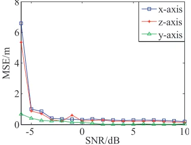
0 2 4 6 8 SNR/dB MSE /m x-axis z-axis y-axis
Figure 5. MSEs under different SNRs.
0.20 0.4 0.6 0.8 0.9 2 4 6 8 10 compressing ratio MSE /m SNR=-6dB SNR=-5dB SNR=0dB SNR=5dB SNR=10dB
little affected by noise, while reconstructedx-axis andz-axis positions are distributed randomly around theoretical values. In order to refine the reconstructed results, curve fitting operation can be applied to the reconstructed positions of each scatterer. After curve fitting operation, the reconstructed position of each scatterer will be a smooth curve. Through independent trials under different SNR values, the mean square errors (MSEs) of reconstructed positions after curve fitting operation compared with theoretical values are shown in Fig. 5. It can be seen that reconstructed x-axis and z-axis positions obtained by interferometric processing are more easily affected by noise than reconstructed y-axis position. When SNR is below −3 dB, the reconstructed positions seriously deviate from theoretical values. Fig. 6 illustrates the relationship of data compressing ratio and MSE of 3-D position with different SNR values. It can be seen that MSE increases with the increasing of compressing ratio. And when compressing ratio is below 0.8, the reconstructed result is relatively accurate.
5. CONCLUSIONS
This paper proposes a 3-D imaging method for high-speed moving space target. Through solving a joint sparsity model with velocity to be estimated, the estimation of velocity is accomplished, and the complex range profile is obtained. No extra velocity compensation is needed. Compared with FrFT based velocity estimation algorithm, the proposed algorithm adopts a sparse sampling mode, thus taking up fewer resources. Meanwhile, the proposed algorithm has a higher accuracy and faster calculation speed. Moreover, the construction of the joint sparse parametric model guarantees the phase coherence of three antennas, which then makes sure that the interferometric 3-D imaging achieve a good result. In general, the proposed 3-D imaging method can compensate the effect of high-speed motion and realize time-varying 3-D imaging of space target, which provides a support for measurement, categorization and recognition of space targets.
ACKNOWLEDGMENT
This work was supported by the National Natural Science Foundation of China under Grant 61571457 and 61631019, the Youth Science and Technology New Star Project of Shaanxi Province under Grant 2016KJXX-49 and the Natural Science Foundation Research Program of Shaanxi Province under Grant 2015JM6306.
REFERENCES
1. Zhang, L., M. D. Xing, C. W. Qiu, and Z. Bao, “Two-dimensional spectrum matched filter banks for high-speed spinning-target three-dimensional IASR imaging,”IEEE Geosci. Remote Sens. Lett., Vol. 6, No. 3, 368–372, 2009.
2. Wang, Q., M. D. Xing, L. G. Yue, and Z. Bao, “High-resolution three-dimensional radar imaging for rapidly spinning targets,” IEEE Trans. Geosci. Remote Sens., Vol. 46, No. 1, 22–30, 2008. 3. Bai, X. R., M. D. Xing, F. Zhou, and Z. Bao, “High-resolution three-dimensional imaging of
spinning space debris,”IEEE Trans. on Geosci. Remote Sens., Vol. 47, No. 4, 2352–2362, 2009. 4. Ai, X. F., Y. Huang, F. Zhao, J. H. Yang, Y. Z. Li, and S. P. Xiao, “Imaging of spinning targets via
narrow-band T/R-R bistatic radars,” IEEE Geosci. Remote Sens. Lett., Vol. 10, No. 2, 362–366, 2013.
5. Luo, Y., Q. Zhang, N. Yuan, F. Zhu, and F. F. Gu, “Three-dimensional precession feature extraction of space targets,” IEEE Trans. Aerosp. Electron. Syst., Vol. 50, No. 2, 1313–1329, 2014.
6. Sun, Y. X., C. Z. Ma, Y. Luo, Y. A. Chen, and Q. Zhang, “An interferometric-processing based three-dimensional imaging method for space rotating targets,” IET 2016 International Radar Conference, 398–402, Guangzhou, China, October 2016.
8. Pang, C. S., T. Shan, T. Ran, and N. Zhang, “Detection of high-speed and accelerated target based on the linear frequency modulation radar,” IET Radar Sonar Navig., Vol. 8, No. 1, 37–47, 2014. 9. Chen, Q. Q., G. Xu, L. Zhang, M. D. Xing, and Z. Bao, “Three-dimensional interferometric inverse
synthetic aperture radar imaging with limited pulses by exploiting joint sparsity,”IET Radar Sonar Navig., Vol. 9, No. 6, 692–701, 2015.
10. Liu, Y. B., N. Li, R. Wang, and Y. K. Deng, “Achieving high-quality three-dimensional InISAR imageries of maneuvering target via super-resolution ISAR imaging by exploiting sparseness,”IEEE Geosci. Remote Sens. Lett., Vol. 11, No. 4, 828–832, 2014.