1141
Volume 66 113 Number 5, 2018
ESTIMATING CROP YIELDS
AT THE FIELD LEVEL USING
LANDSAT AND MODIS PRODUCTS
František Jurečka
1,2, Vojtěch Lukas
1,2, Petr Hlavinka
1,
Daniela Semerádová
1,2, Zdeněk Žalud
1,2, Miroslav Trnka
11 Global Change Research Institute, Academy of Sciences of the Czech Republic, v.v.i, Bělidla 986/4a, 603 00 Brno, Czech Republic
2Department of Agrosystems and Bioclimatology, Mendel University in Brno, Brno, Czech Republic
To cite this article: JUREČKA FRANTIŠEK, LUKAS VOJTĚCH, HLAVINKA PETR, SEMERÁDOVÁ DANIELA, ŽALUD ZDENĚK, TRNKA MIROSLAV. 2018. Estimating Crop Yields at the Field Level Using Landsat and MODIS Products . Acta Universitatis Agriculturae et Silviculturae Mendelianae Brunensis, 66(5): 1141 – 1150.
To link to this article: https://doi.org/10.11118/actaun201866051141
Abstract
Remote sensing can be used for yield estimation prior to harvest at the field level to provide helpful information for agricultural decision making. This study was undertaken in Polkovice, located at low elevations in the Czech Republic. From 2014 – 2016, two datasets of satellite imagery were used: the Moderate Resolution Imaging Spectroradiometer (MODIS) and Landsat 8 datasets. Satellite data were compared with yields and other observations at the level of land blocks. Winter oilseed rape, winter wheat and spring barley yield data, representing the crops planted over the analyzed period, were used for comparison. In 2016, a more detailed analysis was conducted. We tested a relationship between remote sensing data and the spatial yield variability measured by a yield monitor from a combine harvester. Correlations varied from approximately r = 0.4 to r = 0.7 with the highest correlation (r = 0.74) between yield and the Green Normalized Difference Vegetation Index collected from a drone. Vegetation indices from both Landsat 8 and the MODIS showed a positive relationship with yields for the compared period. The highest correlation was between yield and the Enhanced Vegetation Index (r = 0.8) while the lowest was between yield and the Normalized Difference Vegetation Index from MODIS (r = 0.1).
Keywords: crop yield, vegetation indices, remote sensing, satellites, unmanned aerial vehicles, yield estimation
INTRODUCTION
Remote sensing indicators are used in agriculture for monitoring crop conditions and forecasting yield (Wardlow et al., 2012). Indicators widely used in agriculture include vegetation indices (VIs) such as the Normalized Difference Vegetation Index (NDVI) or the Enhanced Vegetation Index (EVI), which track crop progress and evolution in green biomass
of evapotranspiration (ET), which can estimate plant water use (Anderson et al., 2007).
Different spectral bands are used together to derive a dimensionless proxy of plant vitality and standing biomass in the form of VIs. One VI that has been widely used to monitor vegetation conditions, from regional to global scales, is the NDVI (Tucker et al., 1985). Healthy vegetation absorbs most of the visible light that hits it and reflects a huge amount of the near infrared (NIR) light. Unhealthy or sparse vegetation reflects more visible and less NIR bands of the electromagnetic spectrum (Weier and Herring). NDVI is calculated from the visible red (RED) and NIR spectral bands and is expressed by the following formula described by Rouse et al. (1974):
NDVI NIR RED NIR RED
(1)
Calculations of NDVI for a given pixel always result in a number in the range from minus one (–1) to plus one (+1). However, no green leaves give a value close to zero. A value of zero means no vegetation, and a value close to +1 (0.8 – 0.9) indicates the highest possible density of green leaves (Weier and Herring).
A slight modification of NDVI is the Green NDVI (GNDVI). Gitelson and Merzlyak (1998) described in their study that GNDVI was much more sensitive to the changes in chlorophyll concentration than NDVI. It thus allowed the precise assessment of pigment concentration in different chlorophyll variations. Instead of reflectance in the red band, green band (GREEN) is involved in the calculation (Gitelson and Merzlyak, 1998):
GNDVI NIR GREEN NIR GREEN
(2)
Another vegetation index derived from NDVI is the Soil‑adjusted Vegetation Index (SAVI). The SAVI was designed to minimize soil influences on vegetation by introducing a soil‑adjustment factor (L). In the case of SAVI, an adjustment factor is a constant L = 0.5:
SAVI
SAVII NIR RED NIR RED L L
(1 ) (3)
Later, the Modified Soil‑adjusted vegetation index (MSAVI) and its second version (MSAVI2) was developed by Qi et al. (1994) to replace the constant L in the SAVI formula. In the MSAVI formula, the constant L is replaced with a self‑adjusting L. In the case of MSAVI2, an iterative function of L was used in the index derivation:
MSAVI2 2 NIR 1 2 NIR 1 8 NIR RED
2 2
( ( ) ) (4)
Both versions of MSAVI showed good results relating to the vegetation sensitivity and soil noise reduction (Qi et al., 1994).
The EVI was developed as a standard product for the Moderate Resolution Imaging Spectroradiometer (MODIS) sensor on board the polar orbiting Terra and Aqua satellites. EVI provides improved sensitivity in areas with large amounts of biomass (Jiang et al., 2008). The EVI corrects for some distortions in the reflected radiation caused by the particles in the air and the ground cover below the vegetation. The EVI range of values does not become saturated as easily as the NDVI one when rainforests and other areas with large amounts of chlorophyll are observed (Huete et al., 2006). EVI was found to be more linearly correlated with green LAI in crop fields than NDVI (Boegh et al., 2002).
EVI implements the blue band (BLUE) into its calculation in addition to the red and NIR spectral bands (Huete et al., 2002):
EVI x NIR RED NIR xRED xBLUE
2 5
6 7 5 1
. ( )
. (5)
The disadvantage of EVI is its limitation to sensor systems designed with a blue band. The blue band also requires more difficult and varying atmospheric correction schemes that might cause problematic consistency of EVI values (Fensholt et al., 2006).
Therefore, the two‑band EVI (EVI2) was developed by Jiang et al. (2008). EVI2 is calculated only from red and NIR bands without the implementation of a blue band. The idea behind the research activities done by Jiang et al. (2008) was to keep the best similarity with the 3‑band (original) EVI. In this way, EVI2 can be used for sensors without a blue band and at the same time serve as an acceptable substitute of EVI. EVI2 was formulated by Jiang et al. (2008):
EVI2 NIR2 5x NIR REDxRED
2 4 1
. ( )
. (6)
Remote sensing data come from various sources. Many studies have acquired their data from polar orbiting satellites because they are currently freely available. Satellite images often come from the Operational Land Imager (OLI) onboard the Landsat 8 satellite or the MODIS sensor onboard the Aqua and Terra satellites. In 1999, the National Aeronautics and Space Administration (NASA) launched the Terra satellite. In 2002, the Aqua satellite was launched. Aboard both Terra and Aqua sits the MODIS sensor that provides data at spatial resolutions ranging from 1 km to 250 m. Both Terra and Aqua instruments observe the entire Earth’s surface every 1 to 2 days, obtaining data in 36 spectral bands (Johnson, 2014). Landsat 8 was launched in 2013 and provides images of the entire Earth every 16 days. Landsat 8 has 11 spectral bands altogether. Most of the spectral bands are at a spatial resolution of 30 m, while thermal infrared bands are at 100 m and the panchromatic band is at a 15 m resolution (Irons et al., 2012).
In addition to data from polar orbiting satellites, other sources of VIs and other remote sensing indicators can be used, such as airborne imaging and the unmanned aerial vehicle (UAV) surveys by Remotely Piloted Aircraft Systems. UAV platforms are a good alternative to the traditional remote sensing techniques because of their low cost of operation, high spatial and temporal resolution and high flexibility in image acquisition (Zhang and Kovacs, 2012). The main sensing technology in agriculture is based on multispectral cameras, which provide single bands for calculating broadband vegetation indices (Candiago et al., 2015; Gómez‑Candón et al., 2014; Sankaran et al., 2015). The combination of a simple RGB survey with spatial surface models and extracted information of the height of crop biomass resulted in improved crop yield prediction, as shown in the case of the mapping of maize yield by Geipel et al. (2014) and in the estimation of spring barley biomass by Bendig et al. (2014).
There have been studies investigating correlations between various satellite indices and crop yields (Anderson et al., 2016). Conclusions from these studies showed that no single indicator works in all locations at all times because performance depends on many factors such as climate, soil, management, crop type, growing season or the limitations of a given device or sensor (Johnson, 2014).
Our paper provides a comparison of remote and ground‑sensed VIs with yields of three different crops planted in the experimental site – winter wheat (Triticum aestivum L.), spring barley (Hordeum vulgare) and winter oilseed rape (Brassica napus). Altogether, these crops cover the highest planted area of field crops in the Czech Republic (https:// www.czso. cz). They represent crops with different timings of growing seasons (winter vs. spring crop), which cause different levels of moisture sensitivity (Hlavinka et al., 2009; Trnka et al., 2012).
The goal of this paper is to test various indices from different sources to identify suitable remote sensing tools for yield estimation prior to harvest at the field level. The paper also describes the ability of remote sensing products to reproduce the spatial variability of crop yields within the field.
MATERIALS AND METHODS
Experimental site
The experimental site in Polkovice (49°23′50.05″N, 17°14′52.25″E) is located at low elevations (approximately 200 m a.s.l.) with intensive crop production. Polkovice is a village located in the Olomoucký region in the eastern part of the Czech Republic. The site is divided into two land blocks – Niva (26.08 ha) and Trávník (24.38 ha). The soil type at the Polkovice site is chernozem. The experimental site is surrounded by a mosaic of agricultural crop fields dominated mainly by spring barley, winter wheat, winter oilseed rape, sugar beet and maize fields.
The overall climate of the area of the experimental site is influenced by the penetration and mingling of ocean and continental effects. The experimental site is characterized by prevailing westerly and northwesterly winds with rather low precipitation rates. Mean annual temperature for the period 1961 – 1990 is 8.7 °C and mean annual sum of precipitation is 555 mm. In the year 2014, the mean annual temperature was 11 °C and the annual precipitation reached 539 mm. In 2015, the mean annual temperature was 10.7 °C and the annual precipitation was 397 mm. In 2016, the mean annual temperature reached the value of 10.1 °C while the annual precipitation was 461 mm. Weather data come from the weather station situated within the experimantal site.
This data shows that all three years were warmer and drier than the long‑term mean over the period 1961 – 1990. Comparison with long‑term mean shows that especially the year 2015 was very dry with its 397 mm per year. There was relatively low rainfall during July and no rain at all for the middle of August. A heavy rain came on 17th of August
and lasted for three days (17th – 19th of August)
determining the beginning of period with more frequent rains (Pozníková, 2016).
Crop characteristics and yield data
levels. In this study, we focused on yield estimation at the field level. Such a detailed analysis is not commonly available and used in the Czech Republic.
For the period from 2014 – 2016, yield data were available for two land blocks – Niva and Trávník. Data were obtained by grain weighing directly after harvesting by the combine harvester. Standard water content of grains was considered (i.e. 14 % for cereals and 6 % for winter oilseed rape). For the year 2016, harvest was carried out with the combine harvester Claas Lexion 770equipped with a yield monitor and GPS that enabled it to acquire grain flow and moisture records in a 1 s interval. Yield data were filtered in the GIS for erroneous values and processed by ordinary spatial interpolation via kriging into raster format with a spatial resolution of 5 m per pixel.
There were different crops planted in Polkovice over the study period: in 2014, the cultivated crop was winter oilseed rape (Brassica napus); in 2015, it was winter wheat (Triticum aestivum L.); and in 2016, it was spring barley (Hordeum vulgare). Yields were originally reported in tons per hectare, but for the index‑yield comparison for 2014 – 2016, yield data were converted into cereal units.
Remote sensing by satellite data
For 2014 – 2016, remote sensing data were collected from the Moderate Resolution Imaging Spectroradiometer (MODIS) at a spatial resolution of 250 m and from Landsat 8 at a resolution of 30 m. Time series of two indices were used and compared: NDVI and EVI. Index time series were compared over the part of the growing season when changes in vegetation development are most significant and satellite datasets were available (from April to July, except for Landsat 8 in 2014, where the period was from April to the beginning of August). This period was chosen because various studies (e.g., Johnson, 2016) demonstrated that correlations between cereal crop yields and NDVI values peak one or two months prior to harvest. Winter wheat and spring barley were harvested at the beginning of August (6th of August and 8th – 9th of August,
respectively), while oilseed rape was harvested at the end of July and the beginning of August (most of the area was harvested from the 26th of July to
the 2nd of August).
For the MODIS dataset, 16‑day composites from the Terra satellite were used. Composite products help to overcome the impact of cloud cover that can appear on a given day on the quality of satellite imagery. Composites use the data of the best quality over a given period. The 16‑day compositing period was chosen to ensure that pixels were free of noise. Due to this fact, the number of MODIS composites was higher than the available cloudless Landsat scenes. The number of composites varied for every year of the analysis – 10 composites for 2014, 9 for 2015 and 8 for 2016. MODIS composite product MOD13Q1v006 was retrieved from https: / / lpdaac. usgs.gov, maintained by
the NASA EOSDIS Land Processes Distributed Active Archive Center at the USGS / Earth Resources Observation and Science Center, Sioux Falls, South Dakota.
Due to the coarser MODIS resolution, the index value of one representative pixel within each land block was chosen for the index‑yield comparison. This chosen pixel represented typical field conditions and was not influenced by other landscape features, such as roads or forest. Another important criterion was that the chosen pixel did not overlap the land block boundaries. For the Landsat 8 data, the index values obtained depended on data availability that, in turn, depended on the cloudiness of Landsat scenes. Only scenes that did not contain any clouds over the Polkovice site were used. The number of scenes was the same for every year of the analysis – 6 scenes were used per given year. Landsat data from the OLI sensor were downloaded from the Earth Resources Observation and Science (EROS) Center Science Processing Architecture (ESPA) on‑demand interface (https: / / landsat. usgs.gov / espa) run by the U.S. Geological Survey (USGS). Land Surface Reflectance products were downloaded in the form of calculated VIs. The Landsat scenes covering the eastern part of the Czech Republic that included the Polkovice site were used for the extraction of VI values. For the index‑yield comparison, the spatial averages of index values over the land blocks were used.
Unmanned survey and proximal sensing
In 2016, one unmanned survey campaign was carried out over the experimental field with spring barley. The survey occurred on the 7th of June, or
day of year (DOY) 159. For this purpose, the fixed wing Sensefly eBee system was used to collect images via the multispectral sensor MultiSPEC 4C (AIRINOV, France). MultiSPEC 4C consists of a 4‑band optical sensor (green 530 – 570 nm, red 640 – 680 nm, red‑edge 730 – 740 nm and NIR 770 – 810 nm) and a sensor for incoming radiation to normalize light conditions during the flight mission (Haghighattalab et al., 2016). Acquired images were processed in the Pix4D software package (Pix4D SA, Lausanne, Switzerland) to create the final orthomosaic image with a spatial resolution of 0.15 m per pixel.
In addition to the UAV survey, NDVI was measured at 20 points in the field (Fig. 1) with a GreenSeeker handheld crop sensor (Trimble, USA). The amount and location of points was chosen to represent heterogeneity of soil conditions and variability of crop vegetation at the beginning of the growing season in 2016.
as recommended by the producer (www.trimble. com / agriculture). Measurement by the GreenSeeker crop sensor was done four times during the growing season, from May to July. The extraction of all remotely sensed data was done at 20 measurement points in the field where NDVI was measured by the GreenSeeker crop sensor.
Altogether, 9 indices were computed from the UAV survey and the GreenSeeker crop sensor, including NDVI, EVI2, SAVI, MSAVI2, GNDVI and others (Tab. I).
Index‑yield comparison
The ArcGIS (ESRI, USA) and ENVI (Harris, USA) software packages were used for the calculation of indices and the extraction of average values over the Polkovice site. STATISTICA (TIBCO Software, USA) software was used to provide index‑yield correlations for 2016.
First, NDVI and EVI were compared with the average yield data for 2014 – 2016. This was done for both land blocks for the period from the 16th of April to the 30th of June (DOY 106 – 181,
107 – 182 for 2016). This period represents a part of the growing season when changes in vegetation development are most significant. NDVI and EVI sums through the defined period of each year from both satellites were compared with crop yields via regression analyses. Because different crops were planted at the Polkovice site throughout 2014 – 2016, yield data were converted into cereal units (Brankatschk and Finkbeiner, 2014). This conversion allows for the comparison of yields of different crops (e.g., cereals with winter oilseed rape). To achieve a cereal unit from oil seed rape, it is necessary to adjust by a factor of 2 (for winter wheat and spring barley, the factor is 1).
Next, we calculated the detailed VI‑yield correlations for 2016. Dependencies between remote and ground‑sensed data and crop yield were assessed using the Pearson correlation coefficient. Altogether, 10 different indices derived from the UAV, Landsat 8 and the GreenSeeker crop sensor were correlated with spring barley yield in this year (Tab. I).
I: Range of remote sensing data for the study area in Polkovice for the period from 2014 – 2016.
Index Full name of the index Source of data
Landsat 8 MODIS UAV GreenSeeker
EVI Enhanced Vegetation Index 2014 − 2016 2014 − 2016
EVI2 Two‑band Enhanced Vegetation Index 2016
NDVI Normalized Difference Vegetation Index 2014 − 2016 2014 − 2016 2016 2016
NRERI Normalized Red Edge‑Red Index 2016
SRI Soil Reflectance Index 2016
SAVI Soil‑adjusted Vegetation Index 2016
RENDVI Red Edge Normalized Difference Vegetation Index 2016
NDRE Normalized Difference Red Edge Index 2016
MSAVI2 Modified Soil‑adjusted Vegetation Index 2016
GNDVI Green Normalized Difference Vegetation Index 2016
1: Yield map showing the crop variability and measurement points within the experimental site for the year 2016.
RESULTS AND DISCUSSION
The index‑yield comparison for the period from 2014 – 2016 showed a tight relationship between indices and yield data. Fig. 2 shows NDVI and EVI performance during the period from DOY 80 – 220 for individual years of the compared period. VIs from Landsat 8 and MODIS showed different performances, caused by different availability of scenes or composites. VIs from MODIS demonstrated more detailed performance because of the higher frequency of composites, ensuring cloudless imagery within the compositing period.
For Landsat 8, winter wheat and spring barley (years 2015 and 2016, respectively) showed similar relationships and patterns from spring to harvest, with the highest NDVI and EVI values occurring around DOY 140. For the NDVI and EVI values from MODIS, the highest values appeared not only around DOY 140 but also later in the year (around DOY 160 for 2015 and DOY 180 for 2016). For 2014, when oilseed rape was planted at the Polkovice site, the highest index values appeared around or after DOY 160. The NDVI values from MODIS showed one more peak around DOY 100, while index values declined between DOY 100 and 160.
For a better understanding of the relationship between remote sensing data and yields, the yield map was used (Fig. 1). The map is an output of the yield monitor from the combine harvester showing the yield variability within the experimental site. It displays the amount of crop harvested in the particular location in the field in tons per hectare. The map represents the first time that this method has been used at the Polkovice site. Fig. 1 demonstrates that there were higher yields in the Trávník land block than in Niva. Lower values on the left edges of both land blocks may be caused by the shade effect of trees growing along the land block borders.
The NDVI and EVI from both Landsat 8 and MODIS showed a positive relationship with yields for the compared period, even though the index‑yield comparison of indices from MODIS did not show a significant relationship. The Pearson correlation coefficient of the NDVI from MODIS versus yields gave an r = 0.13 for all years, while it gave an r = 0.99 for years 2015 – 2016 (winter wheat and spring barley yields). The correlation of the EVI from MODIS versus yields gave an r = 0.23 for all years and an r = 0.69 for years 2015 – 2016. For the NDVI and EVI from Landsat 8, the differences between the whole period and years 2015 – 2016 were less significant. The correlation showed NDVI performing well, with an r = 0.75 for the whole period and an r = 0.87 for years 2015 – 2016. Furthermore, a correlation of EVI yielded an r = 0.83 for the whole period and an r = 0.99 for years 2015 – 2016.
Linear regressions of scatter plots for the period 2014 – 2016 and the years 2015 and 2016 (Fig. 3)
provide deeper insight into the index‑yield relationships and illustrate the influence of particular crop yields in the overall comparison.
Weak relationships between yields and the indices from MODIS are caused by two factors. First, MODIS has a coarser resolution: 250 m compared to the 30 m of Landsat 8. This resolution is not high enough to provide the proper analysis at such a detailed level (field) and should instead be used for larger areas or larger field blocks. A larger area will better fit the MODIS resolution of 250 m and will probably provide more reasonable results. In this study, only one representative MODIS pixel within each land block was used to attain index values, but more pixels should be chosen to obtain more precise results. Land blocks at the Polkovice site were not large enough to contain more MODIS pixels that would not be influenced by other landscape features (e.g., roads, forest stands, and windbreaks) and simultaneously represent the typical field conditions.
The second factor influencing the performance of both MODIS and Landsat 8 VIs was a seasonal pattern of oilseed rape (planted at the Polkovice site in 2014) that differs from cereals. This factor influenced the performance of VIs from Landsat 8 significantly less than VIs from MODIS. This can be caused by lower amount of available Landsat scenes compared to MODIS composites. The seasonal pattern differs mainly by the earlier flowering date and yellow flowers of oilseed rape. This phenomenon is described in more detail by Johnson (2016), who showed that NDVI values for oilseed rape (from MODIS on Terra and Aqua) achieved the highest values later in the season than the NDVI values for spring barley and winter wheat. The study also showed that the correlation between NDVI and oilseed rape yield peaked much later in the season compared to spring barley and winter wheat. Spring barley and winter wheat obtained their highest correlations in May and at the beginning of June, while oilseed rape correlation values were negative during this period (until the beginning of July). Correlations between oilseed rape yield and NDVI values achieved their highest values in the end of July and in August.
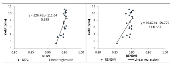
For the year 2016, the correlations between observed spatial variability of spring barley yield and remote and ground‑sensed reflectance data varied mostly from r = 0.4 to r = 0.7 (Tab. II). The correlations between yield and the indices from the UAV were generally high, with the highest correlation (r = 0.74) obtained between yield and GNDVI. High correlations were also found between yield and other indices, such as SRI (r = 0.70) and NDVI (r = 0.69). The relationships between yield data and the VIs (NDVI and RENDVI) from the UAV imagery are shown in scatter plots in Fig. 4. The second highest correlation was found between yield and NDVI, as measured by the GreenSeeker sensor from the 4th of July, 2016
2: NDVI and EVI time series obtained from Landsat 8 and MODIS through part of the growing season for two land blocks over the period from 2014 – 2016.
3: Scatter plots of yield vs. NDVI and EVI obtained from Landsat 8 and MODIS from the 16th of April to the 30th of June (DOY 106 – 181, 107 – 182 for 2016). Correlations of NDVI
and EVI variants to yield are provided for two periods: 2014 – 2016 and 2015 – 2016.
II: Pearson correlation coefficients and coefficients of determination of indices (from the UAV, Landsat 8 and the GreenSeeker sensor) and yield for 2016. Bold values of correlation coefficients are statistically significant at the 0.05 level (p < 0.05).
UAV 7‑Jun‑2016 Landsat 8 GreenSeeker crop sensor
Index r R2 Index Date r R2 Index Date r R2
EVI2 0.403 0.162 EVI 16‑Apr‑2016 –0.102 0.010 NDVI 19‑May‑2016 0.620 0.385
NDVI 0.693 0.481 EVI 9‑May‑2016 0.583 0.340 NDVI 31‑May‑2016 0.497 0.247
NRERI 0.668 0.446 EVI 25‑May‑2016 0.692 0.479 NDVI 23‑Jun‑2016 0.567 0.322
SRI 0.701 0.491 NDVI 16‑Apr‑2016 0.401 0.161 NDVI 4‑Jul‑2016 0.734 0.539
SAVI 0.411 0.169 NDVI 9‑May‑2016 0.676 0.456
RENDVI 0.557 0.310 NDVI 25‑May‑2016 0.638 0.407
NDRE 0.681 0.464
MSAVI2 0.501 0.251
Landsat 8 data was found between yield and the EVI from the 25th of May, 2016 (r = 0.69). The highest
correlation between yield and the NDVI from Landsat 8 was from the 9th of May, 2016 (r = 0.68).
Our paper represents an initial analysis, and further research is needed to better understand the relationships between crop yields and remote sensing products at the field level. Future investigations will include a wider range of remote sensing indices and indicators. One of these will be the two‑band EVI2 to see how EVI and EVI2 perform in comparison with crop yields. It might be useful to see if the utilization of the blue band plays a role. Fensholt et al. (2006) demonstrated that the EVI values might be more problematic due to more difficult and varying atmospheric correction schemes of the blue band. Another remote sensing index that will be included in future studies is the Evaporative Stress Index (ESI), a product of the Atmosphere‑land Exchange Inverse model (ALEXI) (Anderson et al., 2011). ESI is an indicator of agricultural drought expressed as standardized anomalies in the ratio of actual‑to‑potential ET (Anderson et al., 2011, 2013, 2015). The ESI global product is currently at the 5 km resolution, which is too broad for index‑yield comparisons at the field level, as done in this study. A new prototype of the ESI global product with a higher spatial resolution will be available in the near future due to use of the Visible Infrared Imaging Radiometer Suite (VIIRS) sensor on the Suomi NPP satellite (Hain and Anderson, 2017). In addition to classical remote sensing indices, the utilization of LAI can lead to
deeper insights into the index‑yield relationship. A freely available product (MOD15A2H) from the MODIS sensor on Terra combines FPAR and LAI and provides data in an 8‑day compositing period at a spatial resolution of 500 m (https://lpdaac.usgs. gov/dataset_discovery/modis / modis_products_ table / mod15a2h_v006).
In this study, the images from the MODIS on the Terra satellite and Landsat 8 were analyzed for year‑to‑year comparisons of yield data. There are currently more freely available high‑resolution satellite data, such as Sentinels 2A and 2B operated by the European Space Agency since May 2015 (2A). Sentinel multispectral data have great potential, as they are taken at a high spatial resolution of 10 m that better fits with the average size of land blocks in the Czech Republic; the satellite also features a shorter revisit time (3 days for the 2A / B tandem) in comparison to Landsat 8 (16 days).
Another challenge for future investigation is how to analyze the already extracted values of various remote sensing indicators. In this study, NDVI and EVI sums (based on daily VI values derived from linear interpolation between observations) were used to conduct regression analyses. Another option is to utilize polynomial fits of different degrees to imitate the temporal changes in vegetation development (instead of direct lines between observations). In this way, the interpolated values can then be averaged by an arithmetic or weighted (individually for a specific part of the season) procedure over the specified period and compared to crop yields.
4: Scatter plots of yield data and indices obtained from a UAV image from the 7th of June, 2016.
CONCLUSION
In this study, VIs from Landsat 8 and MODIS were compared with yields from two land blocks over the period 2014 – 2016. Correlations of VIs versus yields showed NDVI and EVI from Landsat performing well, while the same indices from MODIS did not show a significant relationship. This was caused by different frequency of Landsat scenes or MODIS composites and different spatial resolution. The 250 m resolution of MODIS compared to the 30 m of Landsat 8 appeared not to be detailed enough to provide reasonable information about yields at a such detailed level. Results of the study showed that the year 2014 was quite problematic due to a seasonal pattern of oilseed rape that is different from cereals. This phenomenon affected more the performance of VIs from MODIS than VIs from Landsat.
approach with the high spatial and temporal resolution useful for site specific crop management. UAV surveys can amend satellite data in yield estimation at such a detailed scale (field) while satellite data can be used for periodic monitoring of crops, even though with low spatial resolution.
Utilization of remote sensing products can be useful for both the field as a whole and for its parts that can by visually assessed as homogenous, and some deviations or stress occurrence could be delimited using VIs from remote sensing. As a non‑destructive method, remote sensing can be utilized several times during the growing season. It can provide crucial information about crop development and be used for real‑time agronomic decision making.
Further investigation is needed for a better understanding of the index‑yield relationships at such a detailed scale. This will include the use of a wider range of remote sensing indicators from different sources at various frequencies and spatial resolutions.
Acknowledgement
FJ, PH and MT were supported by the project SustES – Adaptation strategies for sustainable ecosystem services and food security under adverse environmental conditions (CZ.02.1.01 / 0.0 / 0.0 / 16_019 / 0000797). This work was also conducted at Mendel University in Brno as a part of the project IGA AF MENDELU no. IP 14 / 2016 with the support of the Specific University Research Grant, provided by the Ministry of Education, Youth and Sports of the Czech Republic in 2016.
REFERENCES
ANDERSON, M. C., NORMAN, J. M., MECIKALSKI, J. R., OTKIN, J. A. and KUSTAS, W. P. 2007. A climatological study of evapotranspiration and moisture stress across the continental United States based on thermal remote sensing: 2. Surface moisture climatology. Journal of Geophysical Research, 112(D11): D11112 ANDERSON, M. C., HAIN, C., WARDLOW, B., PIMSTEIN, A., MECIKALSKI, J. R. and KUSTAS, W. P. 2011.
Evaluation of drought indices based on Thermal remote sensing of evapotranspiration over the continental United States. Journal of Climate, 24(8): 2025–2044.
ANDERSON, M. C., HAIN, C., OTKIN, J., ZHAN, X., MO, K., SVOBODA, M. et al. 2013. An Intercomparison of Drought Indicators Based on Thermal Remote Sensing and NLDAS‑2 Simulations with U. S. Drought Monitor Classifications. Journal of Hydrometeorology, 14(4): 1035–1056.
ANDERSON, M. C., ZOLIN, C. A., HAIN, C. R., SEMMENS, K., TUGRUL YILMAZ, M. and GAO, F. 2015. Comparison of satellite‑derived LAI and precipitation anomalies over Brazil with a thermal infrared‑based Evaporative Stress Index for 2003‑2013. Journal of Hydrology, 526: 287–302.
ANDERSON, M., HAIN, C., JURECKA, F., TRNKA, M., HLAVINKA, P., DULANEY, W. et al. 2016. Relationships between the evaporative stress index and winter wheat and spring barley yield anomalies in the Czech Republic. Climate Research, 70(2): 215–230.
BECKER‑RESHEF, I., VERMOTE, E., LINDEMAN, M. and JUSTICE, C. 2010. A generalized regression‑ based model for forecasting winter wheat yields in Kansas and Ukraine using MODIS data. Remote Sensing of Environment, 114(6): 1312–1323.
BENDIG, J., BOLTEN, A., BENNERTZ, S., BROSCHEIT, J., EICHFUSS, S. and BARETH, G. 2014. Estimating Biomass of Barley Using Crop Surface Models (CSMs) Derived from UAV‑Based RGB Imaging. Remote Sensing, 6(11): 10395–10412.
BOEGH, E., SOEGAARD, H., BROGE, N., SCHELDE, K., THOMSEN, A., HASAGER, C. and JENSEN, N. 2002. Airborne multispectral data for quantifying leaf area index, nitrogen concentration, and photosynthetic efficiency in agriculture. Remote Sensing of Environment, 81(2‑3): 179–193.
BRANKATSCHK, G. and FINKBEINER, M. 2014. Application of the Cereal Unit in a new allocation procedure for agricultural life cycle assessments. Journal of Cleaner Production, 73: 72–79.
CANDIAGO, S., REMONDINO, F., DE GIGLIO, M., DUBBINI, M. and GATTELLI, M. 2015. Evaluating Multispectral Images and Vegetation Indices for Precision Farming Applications from UAV Images. Remote Sensing, 7(4): 4026–4047.
DORAISWAMY, P. C., SINCLAIR, T. R., HOLLINGER, S., AKHMEDOV, B., STERN, A. and PRUEGER, J. 2005. Application of MODIS derived parameters for regional crop yield assessment. Remote Sensing of Environment, 97(2): 192–202.
ESQUERDO, J. C. D. M., ZULLO JÚNIOR, J. and ANTUNES, J. F. G. 2011. Use of NDVI/AVHRR time‑series profiles for soybean crop monitoring in Brazil. International Journal of Remote Sensing, 32(13): 3711–3727. FANG, H. L. and LIANG, S. L. 2003. Retrieving leaf area index with a neural network method: Simulation
and validation. IEEE Transactions on Geoscience and Remote Sensing, 41(9): 2052–2062.
GEIPEL, J., LINK, J. and CLAUPEIN, W. 2014. Combined Spectral and Spatial Modeling of Corn Yield Based on Aerial Images and Crop Surface Models Acquired with an Unmanned Aircraft System. Remote Sensing, 6(11): 10335–10355.
GITELSON, A. A. and MERZLYAK, M. N. 1998. Remote sensing of chlorophyll concentration in higher plant leaves. Advances in Space Research, 22(5): 689–692.
GÓMEZ‑CANDÓN, D., DE CASTRO, A. I. and LÓPEZ‑GRANADOS, F. 2014. Assessing the accuracy of mosaics from unmanned aerial vehicle (UAV) imagery for precision agriculture purposes in wheat. Precision Agriculture, 15(1): 44–56.
HAGHIGHATTALAB, A., GONZÁLEZ PÉREZ, L., MONDAL, S., SINGH, D., SCHINSTOCK, D., RUTKOSKI, J. et al. 2016. Application of unmanned aerial systems for high throughput phenotyping of large wheat breeding nurseries. Plant Methods, 12(1): 35.
HAIN, C. R. and ANDERSON, M. C. 2017. Estimating morning change in land surface temperature from MODIS day/night observations: Applications for surface energy balance modeling. Geophysical Research Letters, 44(19): 9723–9733.
HLAVINKA, P., TRNKA, M., SEMERÁDOVÁ, D., DUBROVSKÝ, M., ŽALUD, Z. and MOŽNÝ, M. 2009. Effect of drought on yield variability of key crops in Czech Republic. Agricultural and Forest Meteorology, 149(3–4): 431–442.
HUETE, A., DIDAN, K., MIURA, H., RODRIGUEZ, E. P., GAO, X. and FERREIRA, L. F. 2002. Overview of the radiometric and biopyhsical performance of the MODIS vegetation indices. Remote Sensing of Environment, 83: 195–213.
HUETE, A. R., DIDAN, K., SHIMABUKURO, Y. E., RATANA, P., SALESKA, S. R., HUTYRA, L. R. et al. 2006. Amazon rainforests green‑up with sunlight in dry season. Geophysical Research Letters, 33(6): 2–5.
IRONS, J. R., DWYER, J. L. and BARSI, J. A. 2012. The next Landsat satellite: The Landsat Data Continuity Mission. Remote Sensing of Environment, 122: 11–21.
JIANG, Z., HUETE, A. R., DIDAN, K. and MIURA, T. 2008. Development of a two‑band enhanced vegetation index without a blue band. Remote Sensing of Environment, 112(10): 3833–3845.
JOHNSON, D. M. 2014. An assessment of pre‑ and within‑season remotely sensed variables for forecasting corn and soybean yields in the United States. Remote Sensing of Environment, 141: 116–128.
JOHNSON, D. M. 2016. A comprehensive assessment of the correlations between field crop yields and commonly used MODIS products. International Journal of Applied Earth Observation and Geoinformation, 52: 65–81.
QI, J., CHEHBOUNI, A., HUETE, A. R., KERR, Y. H. and SOROOSHIAN, S. 1994. A modified soil adjusted vegetation index. Remote Sensing of Environment, 48(2): 119–126.
ROUSE, J. W., HASS, R. H., SCHELL, J. A. and DEERING, D. W. 1974. Monitoring vegetation systems in the great plains with ERTS. In: Third ERTS-1 Symposium NASA. NASA SP‑351, Washington DC, pp. 309–317. SANKARAN, S., KHOT, L. R. and CARTER, A. H. 2015. Field‑based crop phenotyping: Multispectral aerial
imaging for evaluation of winter wheat emergence and spring stand. Computers and Electronics in Agriculture, 118: 372–379.
TRNKA, M., BRÁZDIL, R., OLESEN, J. E., EITZINGER, J., ZAHRADNÍČEK, P., KOCMÁNKOVÁ, E. et al. 2012. Could the changes in regional crop yields be a pointer of climatic change? Agricultural and Forest Meteorology, 166–167: 62–71.
TUCKER, C. J., TOWNSHEND, J. R. G. and GOFF, T. E. 1985. African Land‑Cover Classification Using Satellite Data. Science, 227(4685): 369–375.
WARDLOW, B. D., ANDERSON, M. C. and VERDIN, J. P. (Eds.). 2012. Remote Sensing of Drought: Innovative Monitoring Approaches. Boca Raton, FL: CRC Press/Taylor and Francis.
WEIER, J. and HERRING, D. 2000. Measuring Vegetation (NDVI & EVI). NASA earth observatory. [Online]. Available at: https://earthobservatory.nasa.gov/Features/MeasuringVegetation [Accessed: 2018, May 1]. ZHANG, C. and KOVACS, J. M. 2012. The application of small unmanned aerial systems for precision
agriculture: a review. Precision Agriculture, 13(6), 693–712.