The development and evaluation of computer vision algorithms for the control of an autonomous horticultural vehicle

(1)

vision algorithms for the control of an

autonomous horticultural vehicle

J B Southall

A dissertation submitted in partial fulfillment

of the requirements for the degree of

Doctor of Philosophy

of the

University of London.

Department of Computer Science

University College London

(2)

ProQ uest Number: U 643391

INFORMATION TO ALL U SE R S

The quality of this reproduction is d ep en d en t upon the quality of the copy subm itted. In the unlikely even t that the author did not sen d a com plete manuscript

and there are m issing p a g e s, th e se will be noted. Also, if material had to be rem oved, a note will indicate the deletion.

uest.

ProQ uest U 643391

This work is protected against unauthorized copying under Title 17, United S ta tes C ode. Microform Edition © ProQ uest LLC.

ProQ uest LLC

789 East E isenhow er Parkway P.O. Box 1346

(3)

Economic and environmental pressures have led to a demand for reduced chemical use in crop

production. In response to precision agriculture techniques have been developed that aim to increase the efficiency of farming operations by more targeted application of chemical treat

ment. The concept of plant scale husbandry (PSH) has emerged as the logical extreme of preci

sion techniques, where crop and weed plants are treated on an individual basis. To investigate

the feasibility of PSH, an autonomous horticultural vehicle has been developed at the Silsoe Re

search Institute.

This thesis describes the development of computer vision algorithms for the experimental

vehicle which aim to aid navigation in the field and also allow differential treatment of crop

and weed. The algorithm, based upon an extended Kalman filter, exploits the semi-structured

nature of the field environment in which the vehicle operates, namely the grid pattern formed by

the crop planting. By tracking this grid pattern in the images captured by the vehicle’s camera

as it traverses the field, it is possible to extract information to aid vehicle navigation, such as

bearing and offset from the grid of plants. The grid structure can also act as a cue for crop/weed

discrimination on the basis of plant position on the ground plane. In addition to tracking the grid

pattern, the Kalman filter also estimates the mean distances between the rows of lines and plants

in the grid, to cater for variations in the planting procedure.

Experiments are described which test the localisation accuracy of the algorithms in off

line trials with data captured from the vehicle’s camera, and on-line in both a simplified test

bed environment and the field. It is found that the algorithms allow safe navigation along the

rows of crop. Further experiments demonstrate the crop/weed discrimination performance of

the algorithm, both off-line and on-line in a crop treatment experiment performed in the field

(4)

Acknowledgements

Sincere thanks must go to my two supervisors, Bernard Buxton at UCL and John Marchant at

the Silsoe Research Institute, for their advice, encouragement and enthusiasm that has made the

last three years as enjoyable as they have been educational. Danny Alexander read much of this

thesis in draft form, and I thank him for his comments and pertinent questions. Simon Arridge

and S0ren-Aksel S0rensen at UCL, and Andy Frost and Robin Tillett at Silsoe have participated

actively in the various committees set up to monitor my progress over the last three years, and

their comments have been most helpful.

This project would not have been possible without the contributions of a number of people

at the Silsoe Research Institute. Tony Hague has been responsible for the design and develop

ment of the sensing and estimation systems on the autonomous vehicle that the work in this thesis

is centred upon, and it is safe to say that without his efforts the on-line demonstrations presented

here would not have been possible. I also thank Tony for many conversations on the practical

use of Kalman filters, and much of my understanding of the subject is down to him. Ian Jeffs

and Chris Slatcher supervised the growth of the cauliflowers used in experiments throughout this

thesis, and Bob Warded took the photographs of the treated crop seen in chapter 8. His patience

in assembling the mosaics by hand is much appreciated. Simon Miles, John Butler and John

Richards provided much assistance in putting together all manner of bits and pieces of experi

mental equipment.

The members of the image analysis group at Silsoe made me particularly welcome during

my stay in the lab, and I thank them all for their friendship, advice and library code. Dickson

Chan and Robin Tillett risked eye and wrist strain to produce the HUMAN2 and HUMAN3 data

sets seen in chapter 5. Both Tony and John helped me out with field measurements, and John’s

skills as an impromptu milliner saved me from sun-stroke on more than one occasion.

Without the help of my family, my time at university would have been a great deal harder.

So, Mom, Dad and Rachel, thanks for eight years of ’phone calls and visits, and most of all for

supporting me in everything I’ve done for longer than I can remember.

(5)

LOPEX plant spectra data set. The LOPEX data set was established during an experiment con

ducted by the TDP Unit of the Space Applications Institute/Joint Research Centre of the Euro

pean Commission (Ispra). The q h u l l program from the Geometry Centre at the University of

Minnesota was used in the production of the MRROC curves in chapter 8.

(6)

I

o n - li n e ... 100

4.7 S u m m a ry ... 101

5 Off-line and test-bed navigation trials 102 5.1 Off-line ex p erim en ts... 103

5.1.1 Tracking with fixed grid parameters (A U T O )... 104

5.1.2 Tracking whilst estimating grid parameters (A U T 02)...I l l 5.2 Test-bed experim ents... 121

5.2.1 R e s u lts ...123

5.3 S u m m a ry ... 125

6 Initialisation and data association 129 6.1 The initialisation algorithm ... 130

6.2 Data association and validation... 133

6.2.1 Feature validation...135

6.2.2 Implications for filter implementation...136

6.3 S u m m a ry ... 137

7 Image segmentation 139 7.1 The image segmentation algorithm ... 140

7.1.1 Size f ilte r in g ... 140

7.1.2 Feature clustering ...142

7.1.3 Classification summary...145

(9)

7.2.1 The maximum realisable ROC curve... 146

7.2.2 Parameter selection...147

7.3 Segmentation experim ents... 150

7.3.1 Segmentation of ground truth plant matter fe a tu re s ...150

7.3.2 Segmentation of real im a g e s...152

7.4 S u m m ary ... 155

8 Field trials 158 8.1 Position estim atio n ... 158

8.1.1 Experimental r e s u lts ...161

8.2 Crop treatment ... 162

8.2.1 Experimental r e s u lts ...166

8.3 S u m m ary ... 171

9 Conclusions 172 9.1 Localisation... 173

9.2 Plant tre a tm e n t... 174

9.3 Further work ... 175

Bibliography 177

Appendices 189

A The Hough transform row tracker 189

B The matrix inversion lemma 193

(10)

List of Figures

1.1 The Silsoe autonomous horticultural v eh icle... 21

1.2 Vehicle control and navigation architecture ... 22

1.3 The crop row s tru c tu re ... 23

2.1 The grid planting pattern as captured from the vehicle camera... 28

2.2 A flexible template model of the human e y e ... 33

2.3 The grid m o d e l... 34

2.4 The camera and world co-ordinate systems... 35

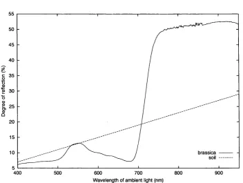
2.5 Reflectance of plant matter and so il... 39

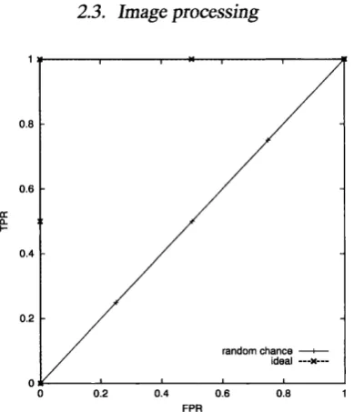
2.6 The ideal and random chance ROC c u rv e s... 42

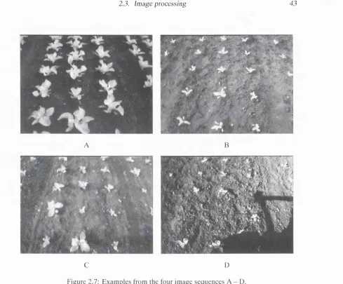
2.7 Examples from the four image s e q u e n c e s... 43

2.8 An image and its plant matter mask ... 44

2.9 The effect of border pixels on classifier performance ... 46

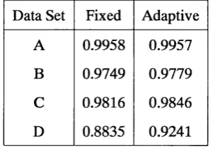
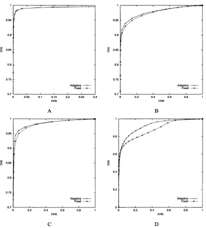
2.10 Experimental results, data sets A - D ... 47

2.11 Example segmentation for sequence A ... 50

2.12 Example segmentation for sequence B ... 51

2.13 Example segmentation for sequence C ... 51

2.14 Example segmentation for sequence D ... 51

2.15 Example segmentation for sequence D with revised cost ra tio ... 52

2.16 An example of chain-coding... 53

2.17 Large plants merge into a single f e a tu r e ... 54

2.18 A plant fractures upon thresholding ... 55

2.19 Projection errors and the virtual ground p l a n e ... 56

4.1 The grid m o d e l... 78

4.2 A comparison between a corruptible and partially incorruptible estimator . . . 92

4.3 Network topologies... 96

(11)

5.1 Trajectories of the state variables for sequence 1 ... 105

5.2 Trajectories of the state variables for sequence 2 ... 106

5.3 A scatter p l o t ... 108

5.4 The Y estimates from AUT02 and SEMI2 for sequence 1 ... 112

5.5 The Y estimates from AUTO and SEMI for sequence 1 ... 113

5.6 Estimated and measured f and / for the first sequence... 113

5.7 Estimated and measured f and

I

for the second s e q u e n c e ... 114

5.8 Estimates from AUTO and A U T 0 2 ...115

5.9 State trajectories whilst estimating the grid parameters, sequence 1 ... 118

5.10 State trajectories whilst estimating the grid parameters, sequence 2 ... 119

5.11 The vehicle in the test-bed environm ent... 122

5.12 The perpendicular offset h ... 123

5.13 Navigation trials... 127

5.14 Estimate uncertainties... 128

6.1 Sampling along a ro w ...131

6.2 A real image sample ... 131

6.3 Comparison of human and automatic assessment of row o f f s e t ...132

6.4 A validation g a t e ... 135

6.5 Order of data incorporation... 137

6.6 Parallel validation... 137

7.1 Blob size h isto g ram s... 141

7.2 The construction of the clustering region Sassoc... 143

7.3 Segmentation schematic ... 145

7.4 Two classifiers and a line in ROC s p a c e ... 146

7.5 A maximum realisable ROC c u rv e ... 147

7.6 MRROC curves for ground truth plant matter segm entations... 149

8.1 Measuring the plant and trail positions... 160

8.2 Navigation trials... 163

8.3 Spray measurement... 165

8.4 Spray treatment results, part o n e ... 168

8.5 Spray treatment results, part t w o ... 169

(12)

List o f Figures 11

8.7 Weed identification, example tw o ... 170

A .l The camera and world plane co-ordinate s y s te m s ... 189

A.2 The crop as seen by the cam era...190

(13)

2.1 Area underneath ROC curves... 46

2.2 Threshold gains a for each image s e q u e n c e ... 50

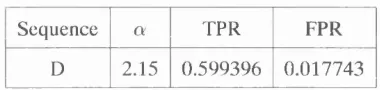
2.3 Threshold gain, TPR and FPR for sequence D ... 52

5.1 Root mean-square differences on the estimate, sequence 1 ... 109

5.2 Root-mean square differences on the Y estimate, sequence 1 ... 109

5.3 Root-mean square differences on the $ estimate, sequence 1 ... 109

5.4 Root mean-square differences on the estimate, sequence 2 ... 110

5.6 Root-mean square differences on the ^ estimate, sequence 2 ... 110

5.7 Filter estimate standard deviations for sequence 1 ... I l l 5.8 Filter estimate standard deviations for sequence 2 ... I l l 5.9 The hand-measured sequence means of f and Ï ... 114

5.10 Root mean-square differences on the tx estimate, sequence 1 ... 115

5.13 Consistency measures on estimates of f, sequence 1 ... 116

5.14 Consistency measures on estimates of /, sequence 1 ... 116

5.15 Root mean-square differences on the tx estimate, sequence 2 ... 116

5.18 Consistency measures on estimates of f, sequence 2 ... 117

5.19 Consistency measures on estimates of /, sequence 2 ... 117

5.20 Estimated standard deviations, sequence 1 ... 121

5.21 Estimated standard deviations, sequence 2 ... 121

5.22 Error measures ...124

(14)

List o f Tables 13

7.1 The area under MRROC curves ... 148

7.2 Operating points for the size filtering and clustering algorithm s... 149

7.3 TPR and FPR for the operating points selected... 150

7.4 TPR and FPR comparison ... 151

7.5 Run A segmentation results... 153

7.6 Run B segmentation results...153

7.7 Run C segmentation results...154

7.8 Run D segmentation results...154

7.9 TPR and FPR ratios for the correctly identified plant matter p i x e l s ...155

8.1 Error measures for outdoor navigation...162

8.2 Measured and estimated forward d is ta n c e ...164

(15)

Introduction

In 1731, Jethro Tull published his book The New Horse Hoeing Husbandry that contained, amongst other innovations, the designs for a device that would lead to the mechanisation of agri

culture. This device was the seed drill, that allowed more orderly and reliable planting of crop

than the traditional broadcasting technique. In broadcasting, the seeds are scattered randomly

across the surface of the soil. Seed drilling deposits the seed on the earth in a regular row and

presses it into the soil where it is more likely to be nourished and is protected from wind, rain

and wildlife. The regular spacing of the rows ensures that the crop plants have approximately

equal volumes of soil from which they can extract nutrients and sufficient access to sunlight, so

each plant grows at a similar pace to its neighbours, and all will be ready for harvest at the same

time.

In addition to its agronomic benefits, the orderly arrangement of crop ensured by the seed

drill paved the way for large scale use of agricultural machines. When seeds were sown by

broadcasting, the resulting irregular positioning of the crop plants meant that weed control had

to be performed by manual hoeing of the field around the plants. Crops planted using the seed

drill grew in rows, which meant that a hoe could be drawn by a horse in straight lines between the

crop rows. Horses were gradually replaced by tractors, and for many crops, mechanical weeding

using a hoe has been replaced by chemical treatment for weed and disease control. Currently,

approximately ^460 million are spent annually on 23,000 tonnes of agro-chemicals in the UK

alone. A rise in consumer interest in organic farming, together with recent controversy over food

crops that have been genetically modified to resist herbicides used in weed control, has led to

pressure to reduce the amount of agro-chemical used in our farms.

Precision agriculture is a concept developed in response to these pressures, where new tech

nology is exploited to achieve the most efficient use of agro-chemicals as possible. Instead of

taking an approach where all of a field is treated with a fertiliser, fungicide or herbicide, the pre

(16)

1.1. Autonomous vehicles 15

the field, according to local requirements. For instance, if a particular region of field was known

to be vulnerable to weed infestation, then more herbicide would be directed toward that region

than to other parts of the same field. The logical extreme of the precision agriculture approach is

the treatment of individual plants. This approach is known as plant scale husbandry (henceforth PSH), and its aim is to direct treatment precisely, with no waste of fertiliser on weeds or soil, or

herbicide on crop [THM96, HMT97b]. The technique may even pave the way to larger scale

organic farming, with precisely guided mechanical weed control.

For PSH to be economically feasible, the treatment systems will almost certainly require

autonomy from direct human supervision. Hague et al [HMT97a] estimate that for precise spray treatment of individual plants, a vehicle carrying the treatment system would be limited to a max

imum speed of approximately lm s~^. This limit is imposed by both real-time computational constraints and physical constraints relating to the time taken to activate a spray treatment sys

tem, and for the spray to reach the plant. Employing a farm worker to drive a vehicle at such

a low speed would be prohibitively expensive, which has prompted scientists at the Silsoe Re

search Institute^ to develop an autonomous horticultural vehicle as a test-bed for experiments in

PSH.

This thesis reports the development and testing of computer vision algorithms designed to

aid both navigation and treatment scheduling for the Silsoe vehicle. The remainder of this intro

duction reviews related work in mobile robotics and provides more detail on the Silsoe vehicle

application, before we outline the contributions presented in this thesis and preview the contents

of the next eight chapters.

1.1 Autonomous vehicles

One of the earliest applications in computer vision was that of autonomous vehicle navigation

in the SHAKEY project which ran at the Stanford Research Institute from 1966 - 1972 [Nil69].

SHAKEY was a mobile robot equipped with bump sensors, a laser triangulation range-finder

and a camera, and was used as a platform for artificial intelligence research into topics such as

object recognition, navigation and path planning in a well-structured indoor environment. Since

this early work, a great deal of research has been performed with autonomous robot vehicles,

and we review some of it below. The work has been partitioned into three categories: indoor

robots, outdoor vehicles and agricultural vehicles. In each case, we concentrate on solutions

which require little or no modification to the system’s working environment.

(17)

1.1.1 Indoor robots

Much of the research conducted into mobile robot navigation has concentrated on indoor ap

plications. The typical scenario is a well-structured indoor space such as an office [SGH"^97],

museum [DFBT99], or factory [BDWH+90]. In these situations, the challenges are localisa

tion, obstacle avoidance and path planning. In our horticultural application, only localisation

is of interest at the moment. Path planning is straightforward as the vehicle must simply fol

low the rows of crop and execute turns at the end of each row to progress to the next. Obstacle

avoidance is not of concern because any evasive action taken in the field is likely to cause dam age to the valuable crop, but obstacle detection will be important in any commercial system to bring the vehicle to a safe halt and prevent accidental damage to the horticultural vehicle (or the

obstruction), and then to alert the farmer that there is something unexpected in the field.

Localisation, the ability to determine one’s position relative to a co-ordinate frame, is vital

for the success of PSH, where the horticultural vehicle must navigate safely in the field and tar

get plant matter for treatment. Many successful mobile robot localisation systems combine both

proprioceptive, or dead-reckoning, information with external views of the world. The combina

tion of the internal and external sensing modalities helps compensate for the weaknesses in each.

The readings from dead-reckoning sensors such as wheel odometry, accelerometers and gyro

scopes are prone to drift, and position estimates from such measurements alone tend to become

increasingly biased away from the true value as the sensor drift increases with time. External

sensors such as sonar, infra-red laser ranging devices and computer vision are prone to outliers

and missing readings, so estimates based upon these alone may be unstable. The combination

of the two sensing modalities corrects for drift in the dead reckoning and allows inappropriate

external sensor readings to be filtered out of the position estimate.

Many successful robots have been constructed using this mixture of sensors. Brady

et al [BDWH+90] describe an incarnation of the Oxford AGV project, designed for moving pallets around factory floors. In their test system odometry is married with a ring of sonar rang

ing devices. The sonar sensors are used to detect range to walls and comers of a room, and these

are matched, where appropriate, to an a priori map of the factory environment [LDW91a]. Sub sequently the methods were transferred to another vehicle [HGB97], where a scanning infra-red

laser was incorporated into the estimation system to provide bearing information to a number

of bar-code targets placed in the robot’s environment from which the robot’s position can be

triangulated^. An overview of the AGV project is given in the book edited by Cameron and

(18)

Probert [CP94].

Crowley [Cro89] describes a sonar-based robot localisation algorithm that bears some sim

ilarity to that of Leonard and Durrant-Whyte [LDW91a], although the features they extract from

the sonar scans differ. Crowley fits line segments to the range readings, whilst Leonard and

Durrant-Whyte search for regions of constant depth (RCDs). RCDs occur “naturally” in sonar

scans, and are typically caused by concave comers in the environment.

The projects mentioned above use pre-determined maps of the environment and the robots

localise themselves with respect to these maps. A more difficult problem is simultaneous map-

building and localisation in unknown environments, which has been attacked using sonar by

Leonard and Durrant-Whyte [LDW91b] and Rencken [Ren93], and with computer vision by

Faugeras and co-workers [AF89, AF88, DF90], Harris [Har92a] and, lately, Davison [Dav98].

All of these approaches [HGB97, LDW91a, Har92a, AF89, Dav98], be they with a priori maps or not, have two common traits. The first is the use of what Leonard and Durrant-Whyte

call geometric beacons as reference points in the world. These beacons may be artificial targets such as the bar-codes read by the laser scanner [HGB97], or distinctive features in the sensed

data, such as RCDs in the sonar scans [LDW91a], comer features in images [Har92a], 3D points,

lines or planes [AF89] or image regions detected by an interest operator [Dav98]. In our horti

cultural application, the regular pattem formed by the crop in the ground is a natural and reliable

beacon that may be used as an aid for localisation.

The second common feature of the work presented above is the use of the Kalman filter al

gorithm to estimate vehicle position and, in the map building applications, beacon position. The

Kalman filter is a recursive estimation algorithm based upon a predict-correct cycle. A model of

the vehicle’s kinematics is used to predict the vehicle’s position after motion has occurred, and a combination of dead-reckoning and extemal measurements are used to correct the predicted position estimate. The Kalman filter algorithm is used in the Silsoe vehicle as outlined below,

and will be treated in greater depth in chapter 3.

1.1.2 Outdoor vehicles

As we have seen, there are valuable lessons to be leamt from indoor navigation schemes, but

there are several additional challenges for autonomous vehicles that operate outdoors. Inside

buildings, the floor is smooth enough that smooth planar motion with no pitch or roll and little

vibration may be assumed, artificial lighting is reasonably constant, and man-made objects typi

cally provide strong features that may be extracted relatively easily from images or sonar scans.

Outside, especially off-road, the ground plane is less reliably flat, there are fewer man-made fea-

(19)

tures, so features extracted from images may be less persistent throughout an image sequence,

and there is no control over natural lighting.

Outdoor vehicles may be separated from those that operate in man-made surroundings, such

as Durrant-Whyte’s automated port container vehicle [DW96] and the many autonomous road

vehicles developed in Germany [Dic98], the USA [TJP97] and Japan [Tsu94], and those vehicles

that operate off-road, such as the AutoNav system [BLD+98], or Camegie-Mellon University’s

various off-road vehicles [LRH94] and the NASA Mars microrover [MS97]. Agricultural vehi

cles are discussed separately in a section below.

The automated highways system (AHS) project has been the focus of much research in

the United States [TJP97, BPT98, MM97]. The AHS project aims to reduce road accidents

and increase traffic flows by placing vehicles under partial or total computer control. The

work at Camegie-Mellon has largely concentrated on problems such as road following and

lane-changing for both automatic vehicle control and driver assistance [TJP97, BPT98]. Such

an emphasis on lateral position estimation and control is typical of much research conducted

into autonomous road vehicles [THKS88, TMGM88, DM96], although McLauchlan and Malik

[MM97] describe a stereo vision system for longitudinal control. In their application, the vehi

cle is part of a “platoon”, a line of cars travelling in close proximity at high speed, and computer

control is required to prevent collision in a situation where human reaction times are too long.

The lateral position sensing in the platoon application is performed by electro magnetic “pick

ups” that sense the position of magnetic nails driven into the road surface at regular intervals. A

full, recent review of road transport automation world-wide is provided by Masaki [Mas98].

Off-road vehicles have a less straightforward sensing task. Road vehicles may take advan

tage of lane markings and road surface modifications (such as magnetic nails) to aid steering

and navigation, whereas off-road autonomous vehicles must determine safe routes for travel in

a much less constrained environment. Dead-reckoning is much more difficult off-road, where

odometry is particularly prone to inaccuracies caused by wheel-slip, and vibration of the vehicle

as it traverses rough terrain adds noise to inertial sensor readings.

Once again, Camegie-Mellon University are leaders in this field, and have developed a

number of off-road vehicles, amongst them the Navlab II vehicle [LRH94] equipped with odom

etry and inertial sensors for position estimation, and a laser range finger for obstacle detection.

Stentz and Hebert describe goal-driven navigation [SH95] where the vehicle is provided with a

map showing its start position and a goal to reach. The vehicle autonomously identifies steerable

routes, marking cells in the map as untraversable, high-cost or traversable depending on whether

(20)

It has been demonstrated at speeds of approximately 2ms~^ over distances of l.ik m .

A second off-road vehicle developed at CMU is the Nomad planetary rover, also equipped with odometry, inertial sensing and a laser range-finder [MSAW99]. In addition to these sensors

it has a differential global positioning system (D-GPS) capability which enabled it to success

fully explore large regions of the Antarctic on an autonomously derived route passing through a

number of human demanded way-points. Carrier-phase D-GPS uses a base station in conjunc

tion with the GLONASS satellite array to derive position estimates, and can be accurate within

a few millimetres, but is very expensive and can suffer from problems with satellite occlusion in

built-up areas, and if communication with the base station is lost, then the system fails, Nebot

and Durrant-Whyte also demonstrate an outdoor autonomous vehicle equipped with a D-GPS

system [NDW99],

Perhaps surprisingly, for our horticultural application we can learn more from the road ve

hicles than those designed for off-road use. The problem of following the rows of crop is closer

to road lane-following than less constrained off-road navigation. For treatment purposes, how

ever, we require precise forward distance estimates, so will be more concerned with longitudinal

direction estimation and control than the autonomous road vehicles research community have

tended to be.

1.1.3 Agricultural Vehicles

The demands of precision agriculture have lead to a number of prototype autonomous agricul

tural vehicles. Yoshida et al [Y0188] describe a vision system for a wheat harvesting vehicle that can follow the border between the stubble left by crop that has been harvested and the un

cut crop. They also detail a system for guidance of a robot in a paddy field, where the vehicle

is guided along the rows of plants by laser and detects the end of each row by locating a target

with an ultrasonic sensor. No details of the accuracy of location estimates or control are given

for either of the two systems.

Another automated harvesting machine, the Demeter automated forage harvester [OS97]

has been developed in the US. Again, they use the line between cut and uncut crop for vehicle

guidance, and are able to use vision to detect the end of the crop rows. No quantitative results

for localisation precision are given, but the harvester has been demonstrated by cutting over 60

acres of alfalfa hay at speeds of 4.5 kilometres per hour (human operators typically drive har

vesters between 3 and 6 kph). The authors intend to integrate a D-GPS receiver into the system

to increase the reliability of the system for cases where the vision algorithms may fail.

Billingsley and Schoenfisch [BS97] demonstrate an automatic guidance system that uses

(21)

Silsoe vehicle). They detect plant matter in colour perspective images of the field collected from

a camera mounted on their tractor, and use regression techniques to fit lines to the crop rows, and

determine the vanishing point of the parallel rows in the image. This information is then used to

provide steering information for the vehicle. They claim that their system is able to steer with

an accuracy of ±2cm with respect to the crop rows, although these figures are obtained from a

test where the vehicle followed a line of white tape along a dark floor.

The agricultural systems outlined above concentrate on guidance for steering control, esti

mating offset and bearing angle to a line, be that line the crop rows [BS97] or the edge of har

vested crop [OS97]. This is a vital component of an autonomous plant scale husbandry system if

it is to navigate along the field without damaging the crop, but we also require accurate longitu

dinal position estimation to allow precise direction of treatment to individual plants. Differential

global positing system receivers are becoming popular in precision agriculture systems [Sta96]

for directing spatially variable field operations^, and they can sense position with an accuracy

of a few millimetres [MF96]. McLellan and Friesen [MF96] claim that accuracy within the re

gion of 2cm will be required for some agricultural operations. However, D-GPS with such high

accuracy is still very expensive and has additional problems such as the relatively infrequent

availability of readings (1 Hz), and can be prone to problems such as satellite dropout, or loss

of communication with the local base station. It was decided not to use D-GPS for navigation

of the Silsoe vehicle, and that longitudinal position would be estimated by dead-reckoning.

1.2 The Silsoe autonomous vehicle project

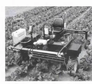
The Silsoe autonomous horticultural vehicle, pictured in a field of cauliflowers in figure 1.1, has

been under development since late 1993 as a platform for the investigation of precise crop and

weed treatment[TMH96]. The vehicle platform started life as a commercially produced manu

ally controlled lightweight agricultural tool carrier, and has been fitted with computer hardware

and sensors (a camera, wheel odometers and accelerometers) to allow autonomous operation in

the field, and a rudimentary treatment system, the spray bar labelled in figure 1.1, for PSH exper

iments. Computing power has been provided by two systems. From 1993 until 1998, processing

was performed by a network of transputers hosted by a laptop PC. In the Winter of 1998/1999,

this rather out-moded hardware was replaced with a single processor Intel Pentium-II system

mnning the Linux operating system, although some transputer hardware has been retained to

perform data collection from the dead-reckoning sensors.

(22)

1.2. The Silsoe autonomous vehicle project 21

Figure 1.1: The Silsoe autonomous horticultural vehicle.

The new work presented in this thesis, started in 1996, extends the capability of the vehi

cle’s com puter vision system, and has built on a considerable volume o f previous effort invested

in developm ent of the vehicle [HT96, MB95, Mar96, PSM97, BM96, SPMB96, RWBM96,

HMT97aJ. The remainder of this section gives details of the autonom ous vehicle and identifies

the problems that the work presented later in this thesis aim to solve.

For autonomous operation, the Silsoe vehicle requires two basic capabilities. The first is

localisation, and the second is the ability to discriminate between the crop, weed and soil. Lo

calisation with respect to some co-ordinate system is required if the vehicle is to navigate itself

in a field of crop, and discrim ination is necessary for the differential treatment of crop, weed and

soil demanded by PSH. We shall treat the two capabilities separately below.

1.2.1 Localisation

Hague and Tillett [HT96] presented the vehicle control and navigation architecture, an amended

and simplified version of which is illustrated in figure 1.2. Many authors are concerned with esti

mating vehicle position relative to an absolute cartesian frame of reference [LDW91a, SSDW95,

BDW H+90], but Hague and Tillet [HT96] argue that a more natural co-ordinate system for op

eration of the Silsoe autonomous vehicle is one that defines position relative to the rows of crop

whose treatment is the focus o f the PSH. The position estimator in figure 1.2, which is a Kalman

(23)

position of the vehicle with respect to the central row of crop plants and the bearing angle of the

vehicle with respect to the central row.

Motor drive signals

-Positional feedback demanded drive

velocities

estimated position error

odometers

accelerometers

vision data wheel velocity control

Path tracking control

Position estimation

Figure 1.2; Vehicle control and navigation architecture.

Odometers and accelerometers are used to generate dead-reckoning estimates of the ve

hicle’s position, velocity and acceleration, with periodic drift correction to the lateral offset

and bearing estimates provided by the computer vision system. The vision system designed by

Marchant and Brivot [MB95], described in detail in appendix A, uses the Hough transform tech

nique [Pra91] to fit a template of the crop row structure to the image, which yields the vehicle’s

lateral offset and bearing relative to the rows. An input image and the fitted row model are pic

tured in figure 1.3. A small number of navigation trials performed by Hague et al [HMT97a] and Hague and Tillett [HT96], both in a test-bed environment and in a field of real crop, show that

error in the estimate of lateral offset is of the order of 8 - 20 m m . Forward position estimates have not been assessed.

The localisation system described above is used only when the vehicle is navigating along

the crop row. At the end of a bed of crop, where a bed is three parallel rows as pictured in fig

ure 1.3, the vehicle must turn and start following the neighbouring bed. The end of each bed

is detected semi-automatically ; the vehicle is given the approximate length of the bed and uses

its estimate of forward motion, and the number of plant matter features detected by image pro

cessing to judge when the vehicle has reached the end of the bed. The vehicle then executes a

pre-programmed turn under dead-reckoning control so that it is in approximately the correct po

sition to travel along the next bed, the vision system starts up again and visually aided tracking

re commences [HMT97a].

1.2.2 Plant recognition

In addition to localisation, a vehicle that performs PSH requires the capability to differentiate be

(24)

1.2. The Silsoe autonomous vehicle project 23

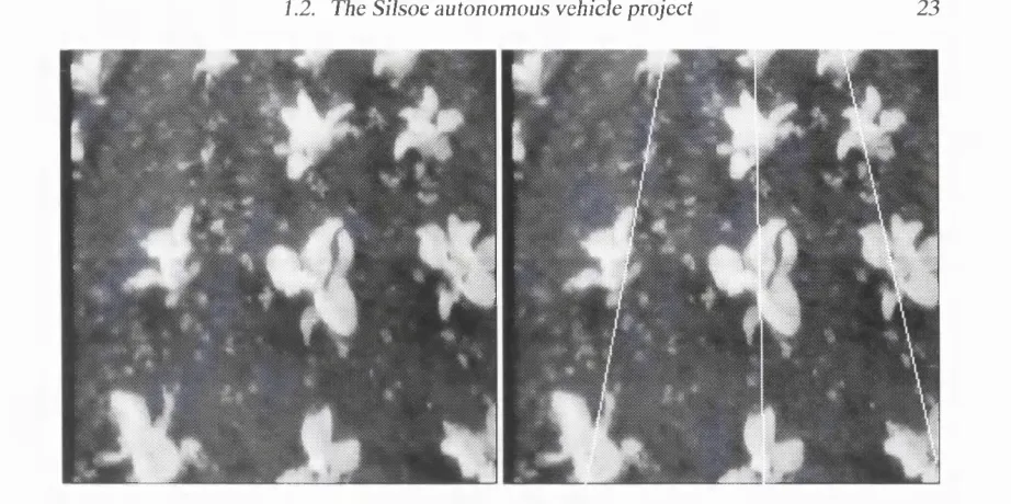
Figure 1.3: The crop row structure. Left: a view of the field from the vehicle’s camera. Right:

the crop rows as located by the Hough transform algorithm due to M archant and Brivot [MB95 ].

and Marchant [BM96] propose candidate algorithm s to separate crop, weed and soil pixels in

monochrome images such as that seen in figure 1.3. The algorithm s use a mixture of hystere

sis thresholding of the pixel grey-levels, techniques from mathematical morphology and grey-

level gradient information. Although they showed promise in off-line trials performed on a desk

top workstation with image sequences captured from the vehicle’s camera, the algorithms have

proved unstable in on-line operation, and are sensitive to changes in illum ination and also to the

size of the crop plants and weeds [ Mar99].

Sanchiz et al [SPMB96] and Reynard et at [RWBM96] present algorithm s for tracking in

dividual crop plants as the vehicle traverses the field. Both algorithm s have been demonstrated

off-line on sequences captured from the vehicle, but have not been implemented for on-line use.

Sanchiz et al model each crop plant as a cluster of “blobs” extracted from the grey-level

image by thresholding, and track the clusters to determine both the motion of the vehicle and

the position of the plants with respect to the vehicle. The algorithm assumes that only image

features that correspond to crop are given to the clustering algorithm , and relied on the method

of Brivot and Marchant [BM96] to correctly provide these features.

Reynard et al ( RWBM96] model the crop plants using contour models [CB92] and demon

strate the robustness of their tracking algorithm to temporary occlusion, as may be caused by

shadows. No method of initialising contours to track particular plants was given, so again, the

(25)

1.2.3 The aims and contributions o f this thesis

The work presented in this thesis aims to extend the capability of the autonomous horticultural

vehicle by introducing a vision algorithm that models the crop pattem as a grid of crop plants rather than a set of rows of plants. We aim to show that this seemingly small change leads to two principal advances:

1. Forward distance estimates may be obtained by a vision algorithm that tracks the crop grid

model. In the original autonomous vehicle navigation system, estimates of forward dis

tance are generated by dead-reckoning alone, and the row model used in the Hough trans

form vision algorithm does not permit estimation of forward motion. Dead-reckoning sys

tems are prone to accumulating errors that lead to biased position estimates, and problems

with wheel-slip can lead to unreliable odometer measurements in the field. It is hoped that

the addition of vision estimates of forward distance will correct for dead-reckoning bias.

2. The crop grid model may be used as an aid for discriminating between crop and weed

plants. For reasons we shall outline in chapter 2, discriminating between crop and weed

plants with image processing techniques is a much harder problem than extracting both

weed and crop features from the images. However, if we are successfully tracking the

crop grid, then image features that support the estimate of grid position may be assumed

to be crop plants, and the remainder weeds.

The contributions made toward the autonomous vehicle project by this thesis are centred

upon the development of an algorithm that tracks the crop grid model through image sequences

using an extended Kalman filter. In addition to the advantages offered by a grid model over the

row model, the use of the extended Kalman filter algorithm, described in detail in chapter 3,

allows a more natural integration of the vision system with the vehicle’s position estimator than

was achieved with Marchant and Brivot’s Hough transform algorithm. Furthermore, the Hough

transform algorithm produces quantised estimates of vehicle position, whereas the Kalman filter

tracker provides continuously valued output.

In addition to the full development of two alternative grid tracking algorithms, a method

for crop/weed discrimination is developed that clusters image features under the constraint that

they support the crop grid model. The use of this algorithm leads to the segmentation of im

ages into regions of crop, weed and soil. The classified image features may be used to guide the

application of treatment.

Each algorithm is implemented for off-line testing on a desk-top workstation, and perfor

(26)

1.3. Thesis outline 25

part of the closed loop control of the autonomous vehicle. The off-line and on-line implementa

tions differ for practical reasons, and these differences are discussed fully before both tracking

and segmentation algorithms are demonstrated in the field with real crop.

On a more theoretical note, we discuss the implications of the control theoretic concepts of

observability and controllability for systems whose state is estimated by Kalman filters. A novel

test for the observability of an extended Kalman filter is derived and the concept of “corruptibil

ity” introduced, which is analogous to controllability for systems with stochastic inputs.

1.3 Thesis outline

The development and testing of the tracking and segmentation algorithms is broken down into

seven chapters. The first of these, chapter 2, introduces the crop grid model and discusses the

perspective imaging of the crop through the vehicle’s camera. Two thresholding algorithms are

proposed for extracting plant matter features fi’om the image data, and their performance com

pared across a set of test images using receiver operating characteristic analysis, which also aids

the selection of an operating point for the preferred thresholding algorithm.

The recursive Kalman filter estimation algorithm, and the related extended Kalman filter,

are discussed in chapter 3. We define and discuss the issues of controllability and observability

and their implications for Kalman filtering. Corruptibility is defined, and a novel test for the

observability of extended Kalman filters derived.

The details of the extended Kalman filters implemented in this thesis are given in chapter 4.

The process and observation models for the off-line implementations are given, and the transfer

to the on-line system discussed. The filters are analysed in terms of their corruptibility and ob

servability. The off-line tracking algorithms are demonstrated in chapter 5, together with initial

navigation trials of the on-line system in a simplified indoor test-bed environment.

In chapter 6, we address two practicalities that are important when using extended Kalman

filters: initialisation and data association. The extended Kalman filter is a recursive algorithm

where the latest estimate of the state of a process is a combination of the previous estimate and

some measurements of the process of interest. The purpose of filter initialisation is to ‘boot

strap’ the recursion with an initial estimate of the vehicle’s location relative to the crop grid that

will subsequently allow successful tracking. Data association techniques are required to extract

appropriate features from the image data to use in estimating the crop grid position. Feature

validation is also discussed.

Whilst chapters 4 and 5 concentrated on the use of the crop grid model as a cue for naviga

(27)

rithm is tested on image sequences captured from the vehicle at different stages of crop growth

and in differing weather conditions.

Two final experiments are presented in chapter 8, where the navigation and crop/weed dis

crimination algorithms are tested on a bed of real crop. Quantitative analysis of the on-line sys

tem’s navigation performance and spray treatment precision is given, and a qualitative analysis

of crop/weed discrimination.

We close with chapter 9, which reviews the results of our experiments and discusses their

(28)

Chapter 2 Image processing in the field environment

In chapter 1, we introduced the Silsoe autonomous vehicle project as a test-bed for experiments

in plant scale husbandry. The vehicle is equipped with a computer vision algorithm that uses

a model of the rows of crop plants [MB95], in conjunction with a dead-reckoning estimator, to

provide localisation information that allows the vehicle to navigate along the rows of crop plants

in the field. In this thesis, we propose that using a crop grid model allows additional localisation

information to be derived from the images (in the form of forward distance estimates) and also

aids crop/weed discrimination.

In this chapter, we review modelling techniques in computer vision to help us specify a

model of the crop grid structure. The crop is viewed through a camera mounted on the front of

the vehicle, and the perspective imaging of the scene is discussed, and formulae are presented

which relate the ground plane position of the crop grid to the locations of crop plants in the image.

We also discuss the processing of the images captured by the camera. To locate the crop grid

model, it is necessary to extract the crop plant features from the image. In plant scale husbandry,

we aim to treat weeds as well as (but in a different manner to) crop, so it is necessary to extract

all plant matter from the image. Two grey-level thresholding algorithms are proposed for this

purpose, and their performance on images collected from the vehicle is analysed using receiver

operating characteristic curves. This method allows both overall performance comparison and

a solution to the problem of operating point selection.

2.1 The semi-structured field environment

As noted in chapter 1, the field environment in which the autonomous vehicle operates contains

a natural “beacon” to navigate by in the form of the crop grid planting pattern. For agronomic

reasons the crop, which in the examples given throughout this thesis is cauliflower, is planted in

a grid structure which allows each individual plant space to grow and access to a region of soil

(29)

transplant them into the soil at a later date. This planting process is performed mechanically by

a transplanter, which places the seedlings on an approximately regular grid, a perspective view

of which can be seen in figure 2.1. This approximate structure, imposed on the world by the crop

planting can serve as a cue for the two aims of vehicle control:

Navigation: the structure provided by the crop grid pattern may be used as a beacon to

localise the vehicle relative to the crop. This localisation serves as an aid to the dead-

reckoning system for vehicle navigation.

Treatment: the knowledge that crop plants are arranged in this grid structure may be used

to discriminate between crop and weeds. Crop plants should lie within the grid structure

where they were planted, whilst weeds will usually grow elsewhere, both because they

tend to grow at random and because they will not thrive if germinating close to a well

established seedling.

Figure 2.1: The grid planting pattern as captured from the vehicle camera.

The image in figure 2.1 has been taken from a sequence captured from the camera mounted on the

vehicle. By using models of the grid structure and the motion o f the vehicle, this grid structure

will be tracked as the vehicle traverses the field. The following sections discuss object m odelling

in machine vision, whilst the problem of tracking receives attention in chapter 3.

2.1.1 Model based tracking in machine vision

Model based tracking is a powerful method of reducing the computational load on an image-

processing system. Rather than analysing all of a static image and categorising each object in it

separately, a model-based tracker aims to ‘lock o n ’ to a specific object or objects in an image se

(30)

2.1. The semi-structured üeld environment 29

object(s) to track it (them) throughout the sequence. Several different types of model have been

proposed [Har92b, CTCG92, YCH89, Low90, BCZ93] with varying degrees of flexibility and

rigidity, and it is important that an appropriate one is chosen, in order to capture the variability

within the class of shapes modelled without introducing extraneous degrees of freedom. Sub

sequent sections review different modelling schemes that are popular in machine vision whilst

bearing in mind that the task at hand is to model the grid structure of the crop planting pattern.

2.1.2 Active contour models

A popular technique used in many tracking applications in machine vision is based upon the ac

tive contour model (ACM). Originally proposed by Kass et al [KWT87], the ACM, or “snake”, is a string of control points, coupled by an elastic material having tension and stiffness properties,

which performs a local search in an image for features such as edges. In its original formulation,

the snake is said to have converged when the “forces” caused by the internal stiffness and tension

balance those derived from the edge features in the image. A drawback of the snake algorithm

is that it requires a good initial configuration close to the required edge, otherwise it will simply

relax to a straight line. The original tracking mechanism for the snake relied on small inter-frame

motion. The predicted position of the snake in the next image of a sequence was simply the posi

tion at which the snake had converged in the current image. Later, more sophisticated predictive

motion models were incorporated into the tracking mechanism [TS92, Bau96].

The idea of joining the ends of the contour to form a closed loop, or “balloon” with an added

pressure force was then proposed [SWHB90, Coh91]. The pressure force makes the balloon

expand until it meets a strong edge, so the initial position is no longer so critical. Also, owing to

the internal smoothing forces, the balloon will ignore weak edges that may be caused by image

noise. A further development of the balloon model is the statistical snake. This is an active

region model (ARM) [IP94], which allows adaptive control of the pressure force to encourage

the snake expand or contract in order to surround regions of an image conforming to a statistical

model. This particular technique has been successfully applied to segmentation and tracking

of road and track regions using statistical colour models [Ale98] and also to colour and texture

segmentation [ZLY95].

The ACM incorporates a very simple shape model where the object of interest is a smoothly

bounded region of the image enclosed by a perimeter of edge features. Such a model is sensi

tive to clutter in the image. A more robust tracker that is less sensitive to clutter could be re-

ahsed if the shape of the contour were further constrained to be specific to a particular class of

objects. Curwen and Blake [CB92] describe such a method, where a B-spline ACM^ (or “dy-

(31)

namic contour”) is coupled to a template such that, in the absence of image forces, the contour’s

shape is that of the template. This biases the contour to lock on to shapes in the image that are

similar to the template. The models are permitted to deform under affine transformations, and a

Kalman filter (see chapter 3) is used to track the contour position over time (similar motion mod

els and tracking schemes have been proposed by Baumberg for more regular ACMs [Bau96]).

This method was demonstrated to run in real-time on a small network of transputers. Since

publication of the original work [BCZ93], the method has been developed extensively to in

corporate features such as learning the dynamics of the object from training sequences [BIR94],

and also differentiating between changes in object shape in the image that are caused by actual

change of the object shape and apparent changes owing to object motion and change of view

point [RWBM96]. A further development is the C O N DENSA TIO N algorithm [IB96] used as the

estimation mechanism in place of the Kalman filter. The strength of the c o n d e n s a t i o n algo

rithm is that, unlike the Kalman filter which is restricted to the uni-modal Gaussian, it has the

ability to handle multi-modal probability densities, thus enabling multiple hypotheses to be prop

agated through the tracking process. In particular, the capacity to maintain multiple hypotheses

increases the robustness of the tracking process. For example, if the tracker becomes distracted

by clutter in an image, a uni-modal tracker can fatally lose track because its single hypothesis al

lows only one object position to be represented. A multi-modal model, however, allows both the

clutter positions and true object position to be represented, and when the clutter is found not to

satisfy the dynamics of the model, then the true object mode will re-assert itself via propagation

of the distribution through the state evolution model.

Although active contour models have been used for tracking individual plants [RWBM96],

and despite their success in many practical vision systems, active contour models and active re

gion models are not natural candidates for the application at hand, which is tracking the position

of the structure formed by a group of plants. When used to track the outline of an object, the

ACM fits its control points to features (typically edge segments) and presents an interpolated

outline of the object. The ACM method is not well suited to the crop grid tracking application

of interest to this thesis, because the structure to be tracked is not a region or object enclosed by

a boundary, but rather a set of individual crop plant positions.

2.1.3 Point distribution models

The point distribution model (PDM) [CTCG92] represents an object by the position of a set of,

say n, landmark points derived from distinguishing features on its boundary or interior. The model is trained on several images, where landmarks have been specified by hand, which aim

(32)

2.1. The semi-structured ûeld environment 31

to represent typical variations in the object’s appearance. This is usually performed by aligning

the training images using a Procrustes procedure [CTCG92] and carrying out a principal com

ponents analysis on the distribution of the aligned landmark points obtained from the training

images. This determines the mean shape of the object together with vectors describing its statis

tically independent principal models of variation. Only the most significant modes are retained

in the model and those accounting for little variation are ignored in order to limit the number of

model parameters, thereby increasing efficiency and avoiding over-fitting problems.

When coupled with an image feature search strategy, the FDM is known as an Active Shape

Model (ASM). The feature search strategy is a method for fitting the model to a new instance of

the object in an image. In fact, the original ASM paper [CT92] was subtitled “Smart Snakes”,

highlighting the similarities between the ASM and ACMs discussed above, as both can be re

garded as a collection of landmark or control points on an object whose positions are influenced

by various “forces”. In an ACM, the control points are connected by elastic forces and there is

no shape specificity. In the ASM formulation, the landmark point positions are coupled by the

statistics underlying the FDM, which permits only certain modes of shape deformation. Since

it allows the object shape to vary and since the variability may be learnt from example training

data, active shape models have been used in the tracking of many types of biological objects,

such as hands [Hea95], pigs [TOM97], fish [MT97] and flocks of ducks [SBT97]. With its abil

ity to cope with deformations, the FDM/ASM is especially well suited to modelling the changes

of shape caused by object flexibility, but it has also found application in fitting a generic model

of an object to particular types. For example. Ferryman et al [FWSB95] construct a generic car model with basic features such as bonnet and boot of variable size and shape, and then train it

on several different models of car, and use the resulting FDM in a system to lock on to and track

any type of car present in the scene.

Another option would be to use the FDM for the crop grid tracking problem with land

mark points taken as the plant positions, but some care must be taken with the model construc

tion. The Frocrustes alignment procedure described by Cootes et al [CTCG92] uses a similarity ransform (planar translation and rotation) to align the training shapes before the principal com

ponents analysis is performed. In our application, where we image the crop in perspective, a

different transformation is required. Chatteijee and Buxton [CB98] use an affine transformation

in the Frocrustes alignment of examples of the outlines of drivable regions that have been ex

tracted from images of unsurfaced country lanes. Although such an approach has not been taken

in this thesis, it might be possible to use the perspective projection in an alignment scheme prior

(33)

variation in the usual manner. Chatteijee and Buxton also make the observation that the affine

transformations between road surface and camera are not entirely random, because they are de

termined, by driver action, to keep the vehicle on the road. To capture this systematic variation

they also performed PCA on the transformations [CB98].

2.1.4 Rigid models

The planting pattern is an example of man-made structure imposed on the world. The tracking of man-made objects has been the focus of much attention [Ste89, Low90, Har92b]. Such ob jects are often rigid or have simple mechanical internal degrees of freedom and may usually be

represented by CAD-like models. Stephens [Ste89] used a Hough transform method to track an

object grasped by a robot arm. A full 3D model of the object was constructed, together with

a look-up table to indicate which features (points on the object’s edges) should be seen from

particular viewpoints. Although the pose estimates generated by the algorithm were noisy, the

system was quite successful in dealing with occlusions and cluttered backgrounds. It should be

noted that by its nature the resolution of any Hough transform pose estimator is limited by the

quantisation of the Hough accumulator, and also that Stephens’ system had no means of cap

turing the dynamics of the model. The assumption was that there was little inter-frame motion

and that the edge positions could be found in successive frames by local search from their previ

ous locations. Lowe [Low90] extracted edge segments from the whole image and a non-linear

minimisation procedure was used to fit a 3D model onto the image. In this case, both rigid ob

jects and articulated objects with rigid subcomponents were modelled, although no quantitative

analysis of the results was given.

The RAPiD algorithm [Har92b] uses similar models to those of Stephens [Ste89] (points on

object edges, with view graphs to predict occlusions for certain poses) to track aircraft and other

objects. The tracking method employed here is the Kalman filter, and the algorithm produces

high quality pose estimates in image sequences of both real and model objects. The Kalman

filter yields continuous (i.e. unquantised) pose estimates, and also a measure of uncertainty on

the estimate.

Both the RAPiD algorithm and Stephens’ Hough transform method are designed for rigid

objects of ideal shape. The crop grid pattern may be regarded as a rigid structure, because once

the crop is planted it is fixed in position. However, the feature points (i.e. the crop plants) should

be allowed to occupy non-ideal positions owing to the variability in the planting process. Any

model of the grid structure should allow for this uncertainty on individual plant positions, which

(34)

2.2. Modelling and viewing the grid structure 33

2.1.5 Flexible templates

The flexible template [YCH89] is a relatively simple idea. A parameterised model of the object

of interest is constructed, and the parameters are varied so as to fit the model to the image. Yuille

et al [YCH89] introduced the deformable template and applied it to extracting features such as the eyes and mouth from images of human faces. Figure 2.2 illustrates their template for the

eye. All of the labelled parameters are allowed to vary in a scheme which minimises a poten

tial energy defined from the goodness of fit of the model to the image. The model of the crop

Xe

Xc

-P2

Figure 2.2: A flexible template model of the human eye (adapted from Yuille et al [YCH89]).

grid structure presented below bears similarities to both a rigid model and a flexible template,

depending on whether or not its parameters are allowed to vary.

2.2 Modelling and viewing the grid structure

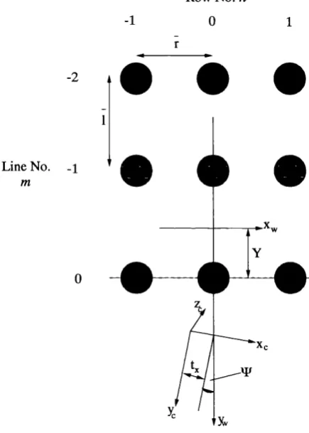
The model of the crop grid pattern is depicted in figure 2.3, where the black circles represent

the ground plane positions of the set of cauliflowers currently in the field of view of the camera.

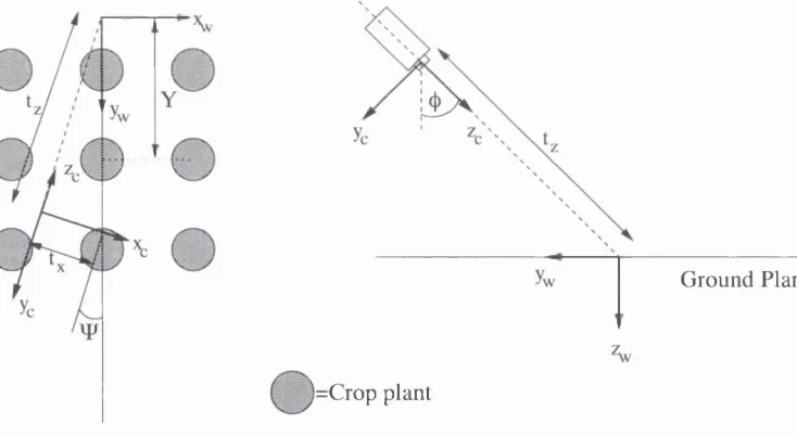
The figure also shows two sets of axes; Vw) is the world co-ordinate frame with the world z axis, z^, projecting into the page, and {xc,yc, Zc) are axes which belong to a co-ordinate system attached to the camera mounted on the vehicle, with describing the camera’s optic axis. Figure

2.4 shows an alternative view that clarifies the relationship between the two co-ordinate frames.

The crop is assumed to lie on the ground plane = 0, and the y^j axis runs through the central row of crop in the field of view. Errors arising from the assumption that the crop lies in the

ground plane are discussed in section 2.3.8 below.

It should be noted that the world co-ordinate frames are local to the vehicle co-ordinate sys

(35)

and crop treatment are carried out by the vehicle, so it is sensible to describe the locations of the

crop and weed in a co-ordinate system relative to the treatment system. As the vehicle moves

across the field, the world axis Xyj axis moves in direct proportion to the distance travelled along the crop rows. A set of co-ordinates is marked on the diagram which specifies the position of

Row No. n

- 1 0 1

r

Line No. _i

Figure 2.3: The grid model.

the vehicle relative to the crop. These co-ordinates are the offset of the optic axis from the

central row of crop, the vehicle’s bearing relative to the central row of crop, and V, which is the offset between the world axis and the bottom-most crop plant in the current image. Y is the co-ordinate which anchors the grid to the vehicle’s co-ordinate system. Two grid param

eters, the mean inter-row spacing f and inter-line spacing

I

(figure 2.3) are used in conjunction with indices m and n to generate the world co-ordinates of the individual plants, as shown in equations 2.1 and 2.2.

Xyj = n x f , (2.1)

yyj = m X I -\-Y- (2.2)

Marchant and Brivot [MB95] (appendix A) presented equation 2.1 in their work on using a

Hough transform to track the row structure. As noted in chapter 1, their algorithm modelled