Article
A Weno-Tvd Implementation for Solving Some
Problems of Hyperbolic Conservation Laws
Jhon Alberto Polo Vásquez1and Miguel Antonio Caro Candezano2
1 Universidad de la Costa; [email protected]
2 Universidad del Atlántico; [email protected]
Abstract:This work deals with a numerical implementation of a fifth order CENTRAL WENO-TVD (Weighted Essentially Non-Oscillatory-Total Variation Dimimishing) scheme [50] applied to the convective terms of some hyperbolic conservation laws problems, in a volume finite framework. The WENO-TVD scheme is used to solve the 1D advection and Burgers equations. For this case is implemented two different numerical fluxes: The Lax-Friedrichs and TVD fluxes. In the TVD fluxes the schemes applied are in flux-limiter form. The schemes implemented for this flux are: Van Albada-1 [44], van Albada-2 [22], van Leer [18] and MINMOD [19]. The WENO type schemes are characterized for their high order approximation, and do not produce spurious oscilations near discontinuities, shocks and higher gradients. A third order Runge-Kutta TVD [13] for the temporal variable is used. Qualitative and quantitative comparison are presented. The numerical solutions are computed with an in-house computer code developed in MATLAB software. In future works, it will develope a paralelization of computer code for solving systems of conservation laws, e.g. Euler equations of gas dynamics.
Keywords: Conservation laws; WENO schemes; finite volume; TVD schemes; numerical flux; flux limiters; Runge-Kutta methods; advection equation; Burgers equation.
1. Introduction
The conservation laws are mathematical expressions of a basic principle that allows to describe the temporal evolution of an amount of interest (temperature, pressure of a fluid, among others). They refer to the physical laws that postulate that during the temporal evolution of an isolated system, where certain magnitudes have a constant value, allowing to preserve the properties of a certain quantity, which can be mass, energy or moment.. Particularly, the hyperbolic laws of conservation describe several physical problems in diverse dynamic areas such as of fluids, astrophysics, shallow water equations, prediction of the climate, compressible gas dymamics, among others. In the face of the need to solve problems in these areas and in turn the lack and/or difficulty of analytical processes for its solution, the numerical methods are used in order to obtain a true approximation to the physical phenomenon.
In order to approximate the conservation laws the finite volume method is used for fluid dynamics problems, with the purpose of studying the conservation of mass u, of some chemical present in a fluid transported by a tube or pipette, withxdistance to the Length of the pipette, for a timet.The MVF subdivide the domain into very small finite parts, called cells or control volumes. This method is based on the fact that many physical laws are conservation laws, suggesting that the input flow of an interest amount, in a cell, is identical to the flow that leaves the adjacent cell. Following this idea, we proceed to formulate the ruling equations in flow conservation equations, defined in an integral way using the averages of cells [9].
To find the solution, we implement the high resolution method WENO (Weighted Essentially Non-Oscillatory) in the convective part, which is based on an interpolation of the average points of cells, standing out for its ability to achieve a high order of precision in smooth regions, it does not
produce oscillatory solutions, maintains the shape in the transition due to contact discontinuities and guarantees convergence.
The first WENO scheme was developed by Liu, Chan and Osher in 1994 [29], which was a finite volume version of third order in a single dimension. In 1996, finite difference schemes of third and fifth order in multispace dimensions were constructed by Jiang and Shu in [21], introducing smoothness indicators and non-linear weights. Then, Shu in 1997, developed [36], ENO schemes (Essentially Non-Oscillatory) and WENO for hyperbolic conservation laws, in 1997. A year later, together with Hu, they developed a scheme WENO for triangular meshes [38]. Harten in [16], introduced the notion of TVD schemes (Total Variation Disminishing) of second order. Later, Titarev and Toro, in 2005, designed [42], an ENO and WENO scheme of second order based on TVDupwind and central fluxs, which is then improved in [49], when using a third-order TVD flow, constructing a fifth-order WENO scheme, developed by Yousef Hashem Zahran in 2006.
This work is framed in the area of numerical analysis and fluid mechanics, as it is intended to undertake a study of the WENO/WENO-TVD schemes of Fifth Order, by implementing a computational code in MATLAB, for the convective part of Hyperbolic conservation laws for the one-dimensional case. For this purpose, the analytical solutions of the working equations, such as the advection and Burgers equations (non-viscous), are compared qualitatively and quantitatively with the numerical solution obtained with WENO/WENO-TVD using the Lax-Friedrichs numerical flux and TVD of third order presented in [49], as well as flow limiters like van Leer [45], van Albada 1 [44], Minmod [32] and van Albada 2 [22]. In order to achieve high-order precision in the temporal discretization, the third-order Runge-Kutta TVD method is used.
This document is organized as follows. In section 2, conservation laws and work equations are studied. In section 3, the numerical methodology of finite volumes, and the types of numerical schemes are discussed in detail. In section 4, the WENO method is explained, based on the ENO reconstruction. Additionally, in section 5 presents the numerical flux schemes, the TVD property and the flux limiter schemes. Time discretization is treated with the Runge-Kutta method in section 6. Finally, in section 7 presents the results in tables and grahps that verify the efficiency of the method.
2. Results
The finite volume method is implemented with a fifth order WENO reconstruction, for the spatial variable, while we use the third order Runge-Kutta TVD method for the time discretization of the problem.
The problems to solve are defined in a spatial domainΩ ⊂ R, considering periodic boundary conditions (PBC) in the given interval, for a determined final timeT. It denotesNas the number of partitions in the size space∆x,Mis the number of time partitions with step∆t, andc = a∆x∆t is the Courant-Friedrichs-Lewy number (CFL), withawave speed.
The schemes to be used are represented as:
WENO-5-LF: Fifth order WENO with numerical flux Lax-Friedrichs. WENO-5-TVD: Fifth order WENO with numerical flux TVD. In addition, the flux limiter is denoted by TVD-3.
2.1. Problem 1
u(x,t):[−1, 1]×[0, 10]→R, ut+ux=0,
u(x, 0) =sen(πx), x∈[−1, 1],
PBCin[−1, 1], T=10, where f(u) =au=u, consideringa=1.
In this problem, the rate of convergence is checked for long times.
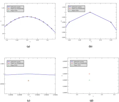
Figure 1.Numerical solution for the advection equation with WENO-5-LF and WENO-5-TVD.N =
100,T=10 andc=0.8(∆x=0.02, ∆t=0.016).
In table1 the results obtained from problem 2.1are presented. In it, it can be seen that the WENO-5-LF and WENO-5-TVD schemes reach an order of precision of the fourth order, in the standardsL1andL∞, even after a long integration time. In addition, it is noted that a higher order
is achieved with the first-order flux of Lax-Friedrichs than with the third-order TVD flux, and that better results are obtained with the normL∞. However, both schemes maintain a minimum of third order.
In the figure2it is shown how the numerical solution adjusts to the exact solution, to the point of not distinguishing itself with the naked eye, due to the small errors obtained in the numerical results. Precisely, an extension of this graph is presented in the figure2, in which the solutions are seen at the pointx≈0.5, allowing to observe that the WENO-5-LF is closer to the solution Exactly the WENO-5-TVD scheme, corroborating that the Lax-Friedrichs flux works better than the TVD flux.
Table 1.Fifth order WENO schemes.T=10,c=0.5. ut+ux=0,u(x, 0) =sen(πx)
Method N ||E||1 p1Order ||E||∞ p∞Order
20 4.2232E-3 3.4141E-3
40 2.5035E-4 4.0763 2.0329E-4 4.0699 WENO-5-LF 80 2.2986E-5 3.4451 1.8215E-5 3.4804 160 2.6109E-6 3.1382 2.0493E-6 3.1519 320 3.1815E-7 3.0368 2.4943E-7 3.0384 640 3.9511E-8 3.0093 3.0980E-8 3.0093
20 3.6529E-3 3.0820E-3
40 2.3131E-4 3.9812 1.9066E-4 4.0148 WENO-5-TVD 80 2.2397E-5 3.3685 1.7762E-5 3.4241 160 2.5925E-6 3.1109 2.0365E-6 3.1246 320 3.1757E-7 3.0292 2.4906E-7 3.0315 640 3.9494E-8 3.0074 3.0977E-8 3.0072
(a) (b)
(c) (d)
Figure 2. Numerical solution of the advection equation at the pointx ≈0.5 with WENO-5-LF and
WENO-5-TVD.N=100,T=10 yc=0.8(∆x=0.02, ∆t=0.016).
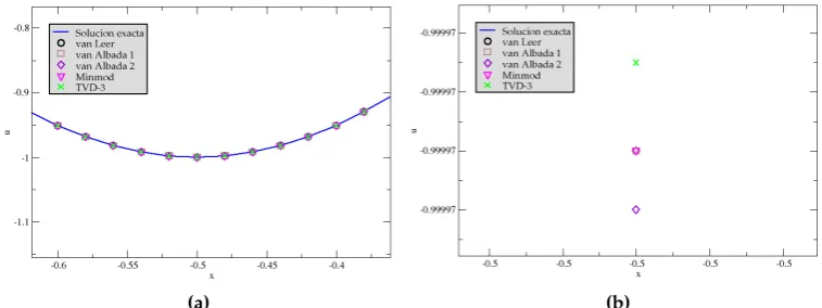
Figure 3.Numerical solution of the advection equation with WENO-5-TVD, using the flux limiter van Leer, van Albada 1, van Albada 2, Minmod and TVD-3. N =100,T = 10 andc =0.8(∆x=0.02, ∆t=0.016).
An extension of the graph3is presented in the figure4 at the pointx ≈ 0.5, in which it can be seen that the flux limiter that works best is van Albada 2, and that in addition the second order limiters present a very similar precision, but still better than the third order TVD limiter.
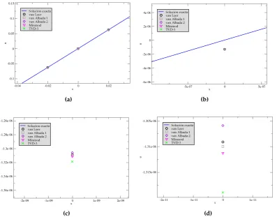
Precisely, a remarkable “difference ” between the flux limiters considered can be seen in the figure5, where the solution at the pointx ≈0 is taken as reference, noting that The best resolution flux limiter is the van Albada 2, followed by van Leer, van Albada 1, Minmod and finally the TVD-3.
(a) (b)
Figure 4. Numerical solution of the advection equation at the point x ≈ 0.5 with WENO-5-TVD,
using the flux limiters van Leer, van Albada 1, van Albada 2, Minmod and TVD-3.N=100,T=10 y
(a) (b)
(c) (d)
Figure 5.Numerical solution of the advection equation at the pointx≈0 with WENO-5-TVD, using
the flux limiters van Leer, van Albada 1, van Albada 2, Minmod and TVD-3. N = 100,T =10 and
c=0.8 (∆x=0.02, ∆t=0.016).
2.2. Problem 2
Let the advection equation (2).
u(x,t):[−1, 1]×[0, 1]→R, ut+ux=0,
u(x, 0) =sen4(πx), x ∈[−1, 1],
PBCin[−1, 1], T=1,
where f(u) =au=u, consideringa=1.
ut+ux=0,u(x, 0) =sen4(πx)
Method N ||E||1 p1order ||E||∞ p∞order
20 9.7475E-2 1.0821E-1
40 8.2671E-3 3.6878 9.1316E-3 3.6953 WENO-5-LF 80 1.0292E-3 3.0601 1.4535E-3 2.6991 160 5.5562E-5 4.2492 5.2160E-5 4.8427 320 5.0982E-6 3.4616 5.3106E-6 3.3109 640 6.1629E-7 3.0014 6.0343E-7 3.0893
20 8.7311E-2 1.0523E-1
40 7.9039E-3 3.5903 9.2198E-3 3.6391 WENO-5-TVD 80 9.3848E-4 3.1296 1.6441E-3 2.5322 160 5.1028E-5 4.2388 4.9789E-5 5.0908 320 5.0861E-6 3.3416 5.2344E-6 3.2644 640 6.1612E-7 2.9984 6.0132E-7 3.0737
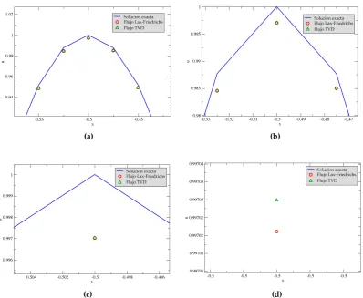
Figure 6.Numerical solution of the advection equation with WENO-5-LF and WENO-5-TVD.N=80,
T=1 andc=0.8(∆x=0.025, ∆t=0.02).
(a) (b)
(c) (d)
Figure 7. Numerical solution of the advection equation at the pointx≈ −0.5 with WENO-5-LF and
WENO-5-TVD.N=80,T=1 andc=0.8(∆x=0.025, ∆t=0.02).
As can be seen in the figure6, there is no deterioration in the accuracy of the solution despite strong oscillations due to the change in the initial condition. It is clear to see, that the numerical solution fits very well to the exact solution both in the valleys and in the crests of the wave.
For instance, at the point x ≈ −0.5, The third-order TVD scheme works better, because the approximate value is closer to the exact value, as shown in the figure7.
2.3. Problem 3
Let the advection equation (2).
u(x,t):[−1, 1]×[0, 10]→R, ut+ux=0,
u(x, 0) =u0(x), x∈[−1, 1],
PBCin[−1, 1], T=10,
u0(x) =
1
6(G(x,z−δ) +G(x,z+δ) +4G(x,z)), −0.8≤x≤ −0.6,
1, −0.4≤x≤ −0.2,
1− |10(x−0.1)|, 0≤x≤0.2,
1
6(F(x,a−δ) +F(x,a+δ) +4F(x,a)), 0.4≤x≤0.6,
0, other case,
whereG(x,z) = e−β(x−z)2,F(x,a) = {max(1−α2(x−a)2)}1/2, taking the constants asa=0.5,
z=−0.7,δ=0.005,α=10 andβ= (log 2)/36δ2.
This problem, better known as the Zalesak problem [51], is used to observe the resolution properties of the scheme, such as the control of oscillations near discontinuities [43].
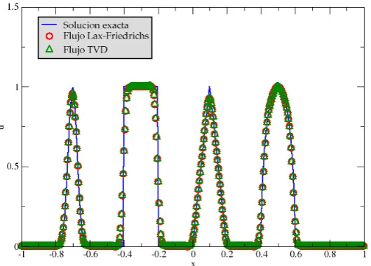
Figure 8.Numerical solution for the advection equation with WENO-5-LF and WENO-5-TVD.N =
200,T=10 andc=0.8(∆x=0.01, ∆t=0.008).
Figure 9.Numerical solution for the advection equation with WENO-5-LF and WENO-5-TVD.N =
In the figures8and9above it can be seen that the solution has no spurious oscillations, since the scheme controls oscillations near discontinuities. Even when the initial soft condition has been changed, by a function in sections, the resolution of the WENO and WENO-TVD scheme remains faithful to the exact solution of the problem, even when it is an initial condition with great variety of shape in its sections. In addition, you can see how the solution improves by takingN=400 instead ofN=200, especially in the non-smooth parts such as the “peaks ”and “”bars.
(a) (b)
Figure 10.Numerical solution for the advection equation at the pointx≈ −0.7 con WENO-5-LF and
WENO-5-TVD.N=400,T=10 andc=0.8(∆x=0.005, ∆t=0.004).
In the first “peaks”of the solution, reached inx ≈ −0.7, a better approximation with the TVD flux is achieved than with the Lax-Friedrichs flux, as can be seen in the figure10.
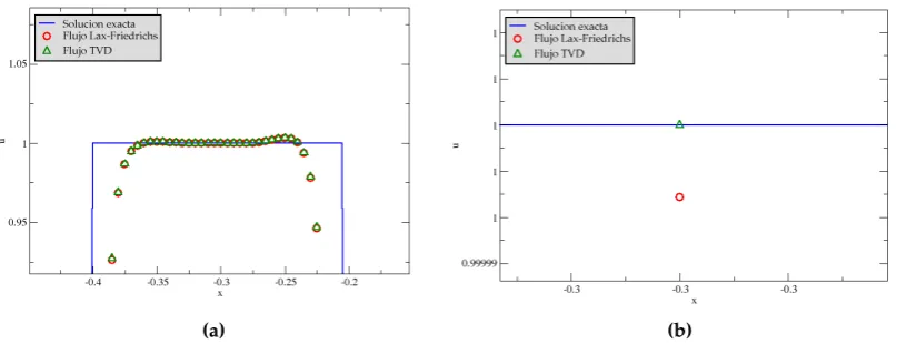
An analogous result is obtained at the pointx≈ −0.3, where a high order of precision is achieved using the TVD flux, in such a way that the numerical solution remains faithful to the exact solution considering a very small scale in the expansion of the graph in the figure9(see figure11)
(a) (b)
Figure 11.Numerical solution of the advection equation at the pointx≈ −0.3 with WENO-5-LF and
(a) (b)
Figure 12. Numerical solution of the advection equation at the pointx≈0.1 with WENO-5-LF and
WENO-5-TVD.N=400,T=10 andc=0.8(∆x=0.005, ∆t=0.004).
In the figure12, we can see once again how the WENO schema works well close to discontinuities and “peaks ”. In this case, we observe the solutions at the pointx ≈0.1, being able to conclude that the flow of Lax-Friedrichs continues to be less precise than the TVD flux, when it comes to this type of graphs.
(a) (b)
Figure 13. Numerical solution of the advection equation at the pointx≈0.5 with WENO-5-LF and
WENO-5-TVD.N=400,T=10 andc=0.8(∆x=0.005, ∆t=0.004).
Finally, when observing the final section of the graph 9 presented in the figure 13, it can be said that it is very similar to the wave crests of the figure1 of problem 1, and as in that case, the monotonous flux of Lax-Friedrichs presents better results in this region of the graph, as occurs for example at the pointx≈0.5.
2.4. Problem 4
u(x,t):[−1, 1]×[0, 1.5]→R, ut+
1 2u
2
x =0,
u(x, 0) =1+1
2sen(πx), x∈[−1, 1], PBCin[−1, 1],
T=0.33 andT=1.5, where f(u) = 12u2.
This problem is used to show the resolution capability of the schemes in the presence of a shock. Two integration times are considered,T=0.33 to show the solution before the shock andT =1.5 to illustrate the solution after the shock which occurs atT=0.5.
Figure 14.Numerical solution for the Burgers equation with WENO-5-LF and WENO-5-TVD.N=80,
T=0.33 andc=0.66(∆x=0.025,∆t=0.015).
(a) (b)
Figure 15.Numerical solution for the Burgers equation at the pointx≈ −0.5 with WENO-5-LF and
WENO-5-TVD.N=80,T=0.33 andc=0.66(∆x=0.025, ∆t=0.015).
In the figures 15 and 16 there are enlargements of the graph (14), which correspond to the solutions (exact and numerical) at the pointsx≈ −0.5 andx≈0, respectively.
(a) (b)
Figure 16. Numerical solution for the Burgers equation at the pointx ≈ 0 with WENO-5-LF and
WENO-5-TVD.N=80,T=0.33 andc=0.66(∆x=0.025, ∆t=0.015).
At both points, it is noted that the Lax-Friedrichs flux works better than the TVD flux, because its graph is closer to the exact solution.
Figure 17.Numerical solution for the Burgers equation with WENO-5-LF and WENO-5-TVD.N=80,
T=1.5 andc=0.66(∆x=0.025, ∆t=0.015).
This is the case, of the intervals[0.1, 0.5]and[0.5, 0.8]in which we can see how the WENO scheme yields better results than the WENO-TVD scheme in the smooth regions of the solution. Otherwise, in the "peaks" and non-smooth regions of the solution, where the WENO-TVD scheme shows better resolution for the nonlinear problem after the shock, as shown in the figures20.
(a) (b)
Figure 18.Numerical solution for the Burgers equation at the pointx≈ −0.3 with WENO-5-LF and
WENO-5-TVD.N=80,T=1.5 andc=0.66(∆x=0.025,∆t=0.015).
(a) (b)
Figure 19. Numerical solution for the Burgers equation in [0.1, 0.5] with WENO-5-LF and
WENO-5-TVD.N=80,T=1.5 andc=0.66 (∆x=0.025, ∆t=0.015).
(a) (b)
Figure 20. Numerical solution for the Burgers equation in [0.5, 0.8] with WENO-5-LF and
WENO-5-TVD.N=80,T=1.5 andc=0.66(∆x=0.025,∆t=0.015).
Figure 21. Numerical solution for the Burgers equation with WENO-5-TVD, using the flux limiters van Leer, van Albada 1, van Albada 2, Minmod and TVD-3. N =80,T =1.5 andc =0.66(∆x=
0.025,∆t=0.015).
(a) (b)
Figure 22.Numerical solution for the Burgers equation atx≈0.6 with WENO-5-TVD, using the flux
limiters van Leer, van Albada 1, van Albada 2, Minmod and TVD-3. N = 80,T =1.5 andc =0.66
(∆x=0.025, ∆t=0.015).
2.5. Figures, Tables and Schemes
List of Figures
1 Numerical solution for the advection equation with WENO-5-LF and WENO-5-TVD.
N=100,T=10 andc=0.8(∆x=0.02, ∆t=0.016). . . 3
2 Numerical solution of the advection equation at the pointx ≈ 0.5 with WENO-5-LF and WENO-5-TVD.N=100,T=10 yc=0.8(∆x=0.02, ∆t=0.016). . . 4
using the flux limiters van Leer, van Albada 1, van Albada 2, Minmod and TVD-3.
N=100,T=10 yc=0.8 (∆x=0.02, ∆t=0.016). . . 5
5 Numerical solution of the advection equation at the pointx ≈0 with WENO-5-TVD, using the flux limiters van Leer, van Albada 1, van Albada 2, Minmod and TVD-3.
N=100,T=10 andc=0.8 (∆x=0.02, ∆t=0.016). . . 6
6 Numerical solution of the advection equation with WENO-5-LF and WENO-5-TVD.
N=80,T=1 andc=0.8(∆x=0.025, ∆t=0.02). . . 7
7 Numerical solution of the advection equation at the pointx≈ −0.5 with WENO-5-LF and WENO-5-TVD.N=80,T=1 andc=0.8(∆x=0.025, ∆t=0.02). . . 8
8 Numerical solution for the advection equation with WENO-5-LF and WENO-5-TVD.
N=200,T=10 andc=0.8(∆x=0.01, ∆t=0.008). . . 9
9 Numerical solution for the advection equation with WENO-5-LF and WENO-5-TVD.
N=400,T=10 andc=0.8(∆x=0.005, ∆t=0.004). . . 9
10 Numerical solution for the advection equation at the pointx ≈ −0.7 con WENO-5-LF and WENO-5-TVD.N=400,T=10 andc=0.8(∆x=0.005, ∆t=0.004). . . 10
11 Numerical solution of the advection equation at the pointx≈ −0.3 with WENO-5-LF and WENO-5-TVD.N=400,T=10 andc=0.8(∆x=0.005, ∆t=0.004). . . 10
12 Numerical solution of the advection equation at the pointx ≈ 0.1 with WENO-5-LF and WENO-5-TVD.N=400,T=10 andc=0.8(∆x=0.005, ∆t=0.004). . . 11
13 Numerical solution of the advection equation at the pointx ≈ 0.5 with WENO-5-LF and WENO-5-TVD.N=400,T=10 andc=0.8(∆x=0.005, ∆t=0.004). . . 11
14 Numerical solution for the Burgers equation with WENO-5-LF and WENO-5-TVD.
N=80,T=0.33 andc=0.66(∆x =0.025, ∆t=0.015). . . 12
15 Numerical solution for the Burgers equation at the pointx ≈ −0.5 with WENO-5-LF and WENO-5-TVD.N=80,T=0.33 andc=0.66(∆x=0.025, ∆t=0.015). . . 13
16 Numerical solution for the Burgers equation at the pointx ≈0 with WENO-5-LF and WENO-5-TVD.N=80,T=0.33 andc=0.66(∆x=0.025, ∆t=0.015). . . 13
17 Numerical solution for the Burgers equation with WENO-5-LF and WENO-5-TVD.
N=80,T=1.5 andc=0.66(∆x=0.025, ∆t=0.015). . . 14
18 Numerical solution for the Burgers equation at the pointx ≈ −0.3 with WENO-5-LF and WENO-5-TVD.N=80,T=1.5 andc=0.66(∆x=0.025, ∆t=0.015). . . 14
19 Numerical solution for the Burgers equation in [0.1, 0.5] with WENO-5-LF and WENO-5-TVD.N=80,T=1.5 andc=0.66 (∆x=0.025, ∆t=0.015). . . 15
20 Numerical solution for the Burgers equation in [0.5, 0.8] with WENO-5-LF and WENO-5-TVD.N=80,T=1.5 andc=0.66(∆x=0.025, ∆t=0.015). . . 15
21 Numerical solution for the Burgers equation with WENO-5-TVD, using the flux limiters van Leer, van Albada 1, van Albada 2, Minmod and TVD-3. N= 80,T =1.5 andc=0.66(∆x =0.025, ∆t=0.015).. . . 16
22 Numerical solution for the Burgers equation atx≈0.6 with WENO-5-TVD, using the flux limiters van Leer, van Albada 1, van Albada 2, Minmod and TVD-3. N = 80,
T=1.5 andc=0.66 (∆x =0.025, ∆t=0.015). . . 16
23 Volumen finito en una dimensión. . . 19
24 Celda solución para el promedio de celdaUn
i.. . . 20
25 Bases “pequeñas" para la reconstrucción enxi+1/2usando tres celdas en cada base. . . 24
26 Flowchart of the WENO scheme to solve LCH 1D. . . 31
List of Tables
1 Fifth order WENO schemes.T =10,c=0.5. . . 4
3 The constantsCrj . . . 23
2.6. Formatting of Mathematical Components
A conservation law is the mathematical expression of a basic principle that allows describing the time evolution of a certain amount of interestu(temperature, pressure of a fluid or the concentration of a chemical, among others) [47].
According [27], a conservation law can be expressed in abbreviated differential form as:
ut+f(u)x=0, (1)
where f is a function ofuand its derivatives, and it’s called theconserved flow of the variables. This project focuses on hyperbolic PDEs and therefore on problems modeled by this type of equations, called hyperbolic problems, particularly working with Hyperbolic Conservation Laws (HCL).
2.6.1. Work equations
1. Advection linear equation
The advection or transport equation describes the advection of the scalar field u(x,t) transported by a constant velocity flowa. Examples of this type of equation are the transport of an atmospheric property, such as humidity, by the effect of wind or the variation of the concentration of a chemical species within a fluid-dynamic current [7]. The equation is given by
∂u ∂t +a
∂u
∂x =0, cona>0. (2)
whereuis the advection rate andais the wave propagation speed [23]. 2. Non-viscous Burgers equation
This equation represents the propagation of weakly non-linear waves in which we can consider one-dimensionality in the spatial variable [7]. The best simplification of the Navier-Stokes equations that preserves the characteristic of having shock waves is given by the hyperbolic EDP of non-viscous Burgers, which is given by:
∂u ∂t +u
∂u
∂x =0. (3)
In this equation the speed of propagation depends on the solution itselfu[23]. 2.7. Finite Volume Method (FVM)
The finite volume method is a numerical method developed by Patankar and Spalding (1972), which allows the resolution of conservation laws. The FVM subdivide the domain into very small finite parts, called cells or control volumes. This method is based on the fact that many physical laws are conservation laws, suggesting that the input flow of an interest amount, in a cell, is identical to the flow that leaves the adjacent cell. Following this idea, we proceed to formulate the governing equations in flow conservation equations, defined using the integral form of a conservation law using the cell averages [9].
Findu(x,t):R×[0,∞)→Rsuch that ux+f(u)x =0, x∈R, t>0, u(x, 0) =u0(x), x∈R,
(4)
Generally, FVM is summarized in the following steps [33]:
1. Discretize of problem domain.
2. Formulation of integral balance equations for each control volume. 3. Approximation of integrals by numerical integration.
4. Approximation of function values and derivatives by interpolation with nodal values. 5. Assembling and solution of discrete algebraic system.
Then, each numeral is expanded.
1. Discretize of problem domain
Let a spatial discretization step∆x > 0 and a time discretization∆t > 0, the sequences are defined
(
xi=i∆x, i∈Z, tn =n∆t, n∈N.
LetΩ⊂Rthe continuous domain of the semi-discrete problem (4).The process of discretization of the domain, consists of decomposingΩin a finite numberN(discrete) of subdomainsIi(i= 1, dots,N), calledcontrol volumes(CVs). This is,
Ω= N
[
i=1
Ii, such asIi∩Ij =∅, ∀i6=j.
For the one-dimensional case as shown in the figure 23, the CVs Ii = [xi−1
2,xi+12] are subintervals of the problem interval, where the edge points of the subintervalsxI±1
2are called
nodos.
Figure 23.Finite volume in one dimension.
In this work, uniform grid are considered, that is, grid in which the size of the cell ∆xi = (xi+1
2 −xi−12)is equal to the spatial discretization step∆x=max1≤i≤N∆xi, this is,∆xi =∆x. 2. Formulation of integral balance equations for each control volume.
For the mean value for integrals, the cell averages are approximate as follows,
Uin≈ 1 ∆x
Z xi+1/2
xi−1/2
u(x,tn)dx≡
Z
Ii
u(x,tn)dx, (5)
where∆x = xi+1/2−xi−1/2is the length of the cell, considering a uniform grid for simplicity
Figure 24.Cell solution for the cell averageUin.
3. Approximation of integrals by numerical integration.
It must be ensured that the numerical method is conservative, thus tracing the natural phenomenon [27]. Then∑ni=1Uin∆x approximates the integral (5) over the entire interval. If the conservative form is used, the flows vary at the extremes of the interval (see figure24), and so by the integral form of the conservation law [27], one has to
d dt
Z
Iiu(x,t)dx= f(u(xi−1/2))−f(u(xi+1/2)). (6) 4. Approximation of function values and derivatives by interpolation with nodal values.
Let the cell averagesUin, in a timetn, we want to approximateUin+1in the next timetn+1, for a
time step∆t=tn+1−tn. Then, integrating (6) fromtntotn+1have
Z
Iiu(x,tn+1)dx −
Z
Iiu(x,tn)dx=
Z tn+1
tn
f(u(xi−1
2,t))dt−
Z tn+1
tn
f(u(xi+1
2,t))dt. (7) Dividing between∆xand clearing we have
1 ∆x
Z
Ii
u(x,tn+1)dx=∆1
x
Z
Ii
u(x,tn)dx− 1
∆x
Z tn+1
tn
f(u(xi+1
2,t))dt−
Z tn+1
tn
f(u(xi−1 2,t))dt
. (8)
5. Assembling and solution of discrete algebraic system. Since (5), the discrete scheme conservatively remains
Uin+1=Uin− ∆t ∆x F
n
i+1/2−Fi−n1/2
(9)
where Fi±n1/2 is the approximation to the average flow in the points x = xi1/2, respectively,
with:
Fi−n 1/2=F Ui−n 1,Uin
, y
Fin+1/2=F Uin,Uin+1
, (10)
For example, the Lax-Friedrichs monotonous flux in the interval[a,b]given by
F(a,b) =1
2[f(a) +f(b)−σ(b−a)]. whereσ=maxu|f0(u)|is a constant [36].
2.7.2. WENO schemes
WENO schemes are high order schemes to approximate the convective part of hyperbolic conservation laws or other partial equations. They are based on high-order reconstruction in order to achieve high precision, not produce oscillatory solutions, preserve the transition form due to contact discontinuities and guarantee convergence [39].
Next, the WENO method is described for the one-dimensional case.
WENO 1D reconstruction procedure
Consider the one-dimensional hyperbolic equation (1) with smooth initial condition. Assuming that the grid is uniform, then solving (1) using a conservative approach to the spatial derivative, we have to
dUi(t) dt =−
1 ∆x
Fi+1 2 −Fi−12
(11)
whereFi±1
2 is the numerical flux andUi(t)are the cell averages in the points(xi,t), which are given by
Ui(t)≡ 1 ∆x
Z x
i+1
2 xi−1
2
u(ξ,t)dξ, i=1, 2, . . . ,N.
A reconstruction procedure consists of obtaining an approximation, for example of a value u(xi+1
2), by means of an interpolation. Initially, consecutive cells should be selected nearxi+12, which should includeIioIi+1. The collection of thesei-cells is called areconstruction stencil.Then, the task is
summarized in finding a single polynomialp(x), at mostk−1 degree, such as the cell average over each cellIiin the stencil, coincides with the averages of given cellsUi, in the pointsxiin the “small" stencil
Sr ={xi−r,xi−r+1, . . . ,xi+s}, (12) forr = 0, 1, . . . ,k−1 withr+s+1 = k, wherer,s ≥ 0 are the number of cells to the left and right, respectively, used in the construction ofSr.
Proposition 1([36]). Given the cell averages of a function u(x):
Ui≡ 1 ∆x
Z x
i+1
2 xi−1
2
u(ξ)dξ, i=1, 2, . . . ,N.
Then there is a unique plynomial pr(x), of degree at most k−1, for each cell Ii, such that it is a k order accurate approximation to the function u(x)inside Ii:
Particularly,
ui+1
2 = pr(xi+12), ui−12 = pr(xi−12), i=1, . . . ,N. (13) When considering the problem (4) with a smooth initial conditionu0(x) =u(x0), andUithe cell
averages of the smooth functionu(x)for each cellIi = [xi−1/2,xi+1/2]for a given order of precisionk,
the WENO reconstruction is based on the ENO interpolation process, which consists of interpolating the functionu, choosing the softer base of kbases considered as defined in (12). Then, a WENO approximation of order 2k−1 to the function u(x) in the bounded cells (u(xi±1/2)), is obtained
according to [36], following the next steps:
1. Obtain thekrebuilt valuesu(i±r)1 2
ofkorder of precision, based in the gridsSrforr=0, . . . ,k−1.
Clearly by the proposition (2.1), there exists a unique polynomial pr(x) of degree at the most k−1, which interpolates the functionu(x), this is,pr(xj) =uj, over the pointsxjin the “small" stencil Sr = {xi−r,xi−r+1, . . . ,xi+s} for r = 0, 1, . . .k−1, with r+s+1 = k. Soon, using u(i+r)1/2 = pr(xi+1/2)like a approximation to the value u(xi+1/2), y u(i−r)1/2 = pr(xi−1/2) like a
approximation to the valueu(xi−1/2), this is,u(xi+1/2) = pr(xi+1/2), yu(xi−1/2) = pr(xi−1/2),
and also because smoothness ofuonSr, we have that:
u(i+r)1/2−u(xi+1/2) =O(∆xk), y
ui−(r)1/2−u(xi−1/2) =O(∆xk).
Now, since theUj are linear in the baseSr, then they are also linear in the pointsui+1/2 and
ui−1/2, therefore there are constantsCrjand ˜Crj, dependent onronSr, such that
u(i+r)1 2
= k−1
∑
j=0
CrjUi−r+j, u(i−r)1 2
= k−1
∑
j=0
˜
CrjUi−r+j, r=0, . . . ,k−1. (14)
Proposition 2([36]). The constants Crjin(14)are given by
Crj =
k
∑
m=j+1 ∑k
l=0
l6=m ∏ k
q=0
q6=m,l
(r−q+1) ∏k
l=0
l6=m
(m−l)
, (15)
if the grid is uniform, for0≤i≤ N,−1≤r≤k−1, y0≤ j≤k−1.
k r j=0 j=1 j=2 j=3 j=4 j=5
1 -1 1
0 1
-1 3/2 -1/2
2 0 1/2 1/2
1 -1/2 3/2
-1 11/6 -7/6 1/3
3 0 1/3 5/6 -1/6
1 -1/6 5/6 1/3
2 1/3 -7/6 11/6
-1 25/12 -23/12 13/12 -1/4 0 1/4 13/12 -5/12 1/12 4 1 -1/12 7/12 7/12 -1/12 2 1/12 -5/12 13/12 1/4 3 -1/4 13/12 -23/12 25/12
-1 137/60 -163/60 137/60 -21/20 1/5 0 1/5 77/60 -43/60 17/60 -1/20 5 1 -1/20 9/20 47/60 9/20 -1/20 2 1/30 -13/60 47/60 9/20 -1/20 3 -1/20 17/60 -43/60 77/60 1/5 4 1/5 -21/20 137/60 -163/60 137/60
-1 49/20 -71/20 79/20 -163/60 31/30 -1/6 0 1/6 29/20 -21/20 37/60 -13/60 1/30 1 -1/30 11/30 19/20 -23/60 7/60 -1/60 6 2 1/60 -2/15 37/60 37/60 -2/15 1/60 3 -1/60 7/60 -23/60 19/20 11/30 -1/30 4 1/30 -13/60 37/60 -21/20 29/20 1/6 5 -1/6 31/30 -163/60 79/20 -71/20 49/20
For instance, whenk = 3, andr = 1 we have the “small" stencilS0 = {xi,xi+1,xi+2},S1 =
{xi−1,xi,xi+1}, S2 = {xi−2,xi−1,xi}, as shown in the figure 25. Then, by the proposition (1) there is a unique polynomialpr(x)such that
1 ∆xi−1
Z xi−1/2
xi−3/2
pr(x)dx=Ui−1,
1 ∆xi
Z xi+1/2
xi−1/2
pr(x)dx=Ui,
1 ∆xi+1
Z xi+3/2
xi+1/2
pr(x)dx=Ui+1.
then by taking u(i+r)1/2 = pr(x) as an approximation of u(xi+1/2), we can write such an
ui(+0)1/2=C00Ui+C01Ui+1+C02Ui+2
= 1 3Ui+
5 6Ui+1−
1 6Ui+2, ui(+1)1/2=C10Ui−1+C11Ui+C12Ui+1
=−1 6Ui−1+
5 6Ui+
1 3Ui+1, ui(+2)1/2=C20Ui−2+C21Ui−1+C23Ui
= 1 3Ui−2−
7 6Ui−1−
11 6 Ui.
These approximations are of third order of precision if the functionu(x)is smooth in the stencil Srwithr=0, 1, 2.
The WENO reconstruction procedure takes a convex combination of the low-order approximations, to achieve a high order approximation at the boundary points, based on a “big" stencil S = {xi−k+1, . . . ,xi+k−1}, which is the union of all the “small" stencils Sr
considered above. The objective is to find a unique polynomial of degree at the most 2k−2, denoted by p(x), interpolating the function u(x)in the points of the “big" stencil. Suppose ui+1/2= p(xi+1/2)as the approximation to the valueu(xi+1/2), we have to
ui+1
2 −u(xi+12) =O(∆x
2k−1), (16)
by virtue of the smoothness of the functionu(x)in the gridS.
Figure 25.“Small” stencils for the reconstruction inxi+1/2using three cells in each stencil.
2. Find the constantsdrand ˜dr, which are called thelinear weights, such that
ui+1 2 =
k−1
∑
r=0
dru(r)
i+12 =u(xi+12) +O(∆x
2k−1) y
ui−1 2 =
k−1
∑
r=0
˜ dru(i−r)1
2
=u(xi−1
2) +O(∆x 2k−1)
are true, withdr, ˜dr ≥0 y∑k−1
d0=1, k=1;
d0= 2
3, d1= 1
3, k=2; d0= 3
10, d1= 6 10 d2=
1
10, k=3; Then, fork=3, we get
ui+1/2= 3
10u (0) i+1/2+
6 10u
(1) i+1/2+
1 10u
(2) i+1/2
= 1
30Ui−2− 13 60Ui−1+
47 60Ui+
9
20Ui+1− 1 20Ui+2. which is an accuracy of 2k−1, but oscillatory [36].
Therefore, if we only want to obtain the order of precision 2k−1, simply choose the linear weightsdr >0 arbitrarily, so that we add one.
3. Then, in order that the approximation be non-oscillatory in shocks, contact discontinuities, high gradients, among others, we change the linear weights by constants omegar, to rewrite this approximation as
ui+1/2=ω0u(i+0)1/2+ω1u(i+1)1/2+ω2u
(2)
i+1/2 (17)
dondeω0,ω1yω2are called thenonlinear weights, such thatωr ≥0 and∑k−r=01ωr =1, which is required to satisfy the following properties:
• Ifu(x)is smooth in all stencilSr, the the nonlinear weights are approximate by the linear weights.
• Ifu(x)has a discontinuity in the basesSr, then the correspondingωrshould be essentially zero, to emulate the idea of ENO.
Combining all these aspects, a robust choice of the nonlinear weights given in [36] is
ωr = αr ∑k−1
s=0αs
y ω˜r= α˜r ∑k−1
s=0α˜s
(18)
withr=0, . . . ,k−1 where theαrare given by
αr= dr
(ε+βr)2 and ˜
αr = ˜ dr
(ε+βr)2 (19)
where ε ∈ [10−5, 10−7] (usually 10−6, [36]) is introduced so that the denominator is different
from zero. The betarare called the textit softness indicators of the baseSr.
4. The smooth indicators measure the degree of smoothness of the functionu(x)in the stencilSr, in such a way that the total variation of the interpolating polynomialpr(x)in Ii [36]. Ifu(x)is smooth in the stencilSr, then
βr =O(∆x2), (20)
while ifu(x)has a discontinuity in the stencilSr, then we get
A definition forβrwhich meets these requirements is given in [36] by:
βr = k−1
∑
l=1
Z x
i+1
2 xi−1
2
∆x2l−1
∂lpr(x) ∂lx
2
dx, con r=0, . . . ,k−1. (22)
For example, computing fork=3, (22) get
β0=13
12(Ui−2Ui+1+Ui+2)
2+1
4(3Ui−4Ui+1+Ui+2)
2, (23a)
β1=13
12(Ui−1−2Ui+Ui+1)
2+1
4(Ui−1−Ui+1)
2, (23b)
β2=13
12(Ui−2−2Ui−1+Ui)
2+1
4(Ui−2−4Ui−1+3Ui)
2. (23c)
5. Finally, we get the WENO reconstruction of 2k−1 order, ofu(x)in the boundary points given by:
uLi+1 2
= k−1
∑
r=0 ωru(r)
i+12, u R i−1 2 = k−1
∑
r=0
˜
ωru(i−r)1 2
, (24)
where the super-index (L)indicates that the base Sis skewed to the left, meaning that more grid points are used to the left ofxi+1
2 to the right, similarly the(R)indicates that the baseSis skewed to the right, by using more mesh points to the right ofxi−1
2 to the left.
2.7.3. Numerical flux schemes
We intend to calculate the approximations of the numerical flowFi+1/2andFi−1/2, in the border
points of the cellIi = [xi−1/2,xi+1/2], for a certain numeric fluxF. The schemes to work are:
• Lax-Friedrichs flux
It is a monotonous central flux of first order, probably the best known and used due to its simplicity. It is given by [37,49]:
FiLF+1/2= 1 2
f(ui) +f(ui+1)
− ∆t 2∆xσ
ui+1−ui
, (25)
whereσ=maxu|f0(u)|. • Third order TVD flux
It is a TVD flux of third order presented in [49], which is given for the linear scalar case by:
FiTVD+1 2
= 1
2[f(ui) +f(ui+1)]− 1
2|a|∆i+12u+|a|{A0∆i+12u+. . . · · ·+A1∆i+L+1
2u}φi+|a|A2∆i+M+12uφi+M
(26)
where
A0=
1 2−
|c|
4 , A1=− |c|
8 − c2
8, A2=− |c|
8 + c2
8, (27)
φi=
(1− |c|)θi
η(A1θi+A0θA2)
, 0≤θi≤θL
1, θL ≤θi ≤θR
1− |c|+ηA2φi+M/θi∗ η(A1θi+A0) ,
θi >θR
0, θi <0,
(28a)
with
φi+M=
η θi+M,i f 0≤θi+M<0.5 1, i f θi+M>0.5 0, i f θi=0,
(28b)
where
θL = η(A0−A2)
1− |c| −ηA1
,
θR= 1
− |c| −η(A0−A2φi+M/θ∗i) ηA1
, (28c)
θi=
∆i+L+1 2u ∆i+1
2u
(28d)
dondeθiis called the local flow parameter and
θ∗i =
∆i+L+1 2u ∆i+M+1
2u
(28e)
is called the upwind-downward flow parameter andηis defined by
η=
1− |c|, i f 0≤ |c|< 1 2
|c|, i f 1
2 ≤ |c| ≤1.
(28f)
Observation 3([49]). For the non-linear case, in the scheme (26), the velocity is a dependent function of u, that is a=a(u), and therefore Roe rates are used [36], defined by:
ai+1/2=
f(ui+1)−f(ui)
ui+1−ui
, if ui6=ui+1
f0(ui), if ui=ui+1,
(29)
and we change a by ai+1/2. In this way, the local flux parameterθiis redefined by
θi =
|ai−1/2|(ui−ui−1)
|ai+1/2|(ui+1−ui). (30)
2.7.4. Limiter flux schemes
problem, sometimes it is not enough, and it is necessary to use flux limiters, which together with an appropriate high resolution scheme, causes the solutions to decrease the total variation (see [18,19,27]).
Total Variation Disminishing property (TVD)
To measure the oscillations in a solution, we define thetotal variation TV(Un)of a functionUas
TV(Un) = N
∑
i=1
|Un
i+1−Uin|, (31)
wherei =1 andi= Nare the boundary to the left and the right of the numerical grid, respectively. [50].
Therefore, a numerical scheme is TVD (Total Variation Disminishing) if:
TV(Un+1)≤TV(Un) (32)
for allnand∆tsuch that 0≤n Deltat≤T. That is, the total variations do not grow over time, so that TV(Un), for anynis bounded byTV(U0)of the initial condition [13].
2.7.5. Flux limiter
The idea is to represent the numerical flux as an additive decomposition of a flux ofunderorder FL (usually some monotone flux) and a flux of highorder FH, such so that F is reduced toFH in smooth regions, or reduced toFLclose to discontinuities [20]. This is,
Fi+1/2=FiL+1/2−φ(θi)
FiL+1/2−FiH+1/2 Fi−1/2=Fi−L1/2−φ(θi−1)
Fi−L1/2−Fi−H1/2
where, φis the limiter flux function, dependent onlocal flux parameter θ (orr in some cases),
defined by:
θi = ∆i−1/2 u ∆i+1/2u
= ui−ui−1 ui+1−ui
, (33)
which represents the radius of the successive gradients in the given cell and measures the smoothness of the solution [15,49].
It is important to note thatφ(θi):=φi≥0. Whenφi =0 (peak gradient, opposite slopes or zero gradient), the flux is represented by low order flux. Analogously, whenφi=1 (smooth solution), the flux obtained is of high order (second order) [15].
φ (θ) =
1+|θ| van Leer, (34)
φva1(θ) = θ 2+θ
θ2+1 van Albada 1, (35)
φva2(θ) = 2θ
θ2+1 van Albada 2, (36)
φmm(θ) =max[0, min(1,r)] Minmod, (37)
donde los limitadores (34), (35) y (37) sonsimétricos, esto es, que cumplen que
φ(θ) θ =φ
1
θ
. (38)
Theorem 4 ([49]). Scheme (9) with the numerical flux (26) is TVD for|c| ≤ 1 if the limiter function is determined by (28).
2.7.6. Time discretization
In this section, time discretization is emphasized, since once the spatial part is worked for an initial time, the idea is to extend this procedure for a following time, which is implemented using a class of high Runge-Kutta methods. order [19], whose objective is to maintain the property TVD (32), when achieving a high order of precision in time [13].
This method is used to solve EDO systems in the same way
ut=L(u) (39)
whereL(u)it is an approximation to the derivative−(f(u)x)in the equation (1).
Analogous to the driscretization in space, we denote the time astn = n·∆t, so that we useUin to denote the approximation to the exact solutionu(x,t)in the mesh points(xi,tn).
The Runge-Kutta methods that comply with the TVD property for some restriction in the CFL, are called Runge-Kutta SSP methods (Strong Stability Preserving) [14], in which the method is assumed from Euler forward is strongly stable, that is,||Un
i −∆tL(Uin)|| ≤ ||Uin||, and it is considered a restriction for the CFL, so that it is satisfied that||Uin+1|| ≤ ||Un
i||(see [13,50]).
According to [13], the third-order Runge-Kutta method TVD is given by
Ui(1)=Uin+∆t L Ui(n)
Ui(2)= 3 4U
(n) i +
1 4U
(1) i +
1 4∆t L U
(1) i
Ui(n+1)= 1 3U
(n) i +
2 3U
(2) i +
2 3∆t L U
(2) i
It is important to remake that even when considering a good second-order spatial discretization TVD, if the temporal discretization is linearly stable but not TVD, then we can obtain oscillatory results (see [13]). Therefore it is suggested to use Runge-Kutta TVD/SSP methods for hyperbolic problems [14].
3. Discussion
In this work a WENO/WENO-TVD implementation was performed using the Lax-Friedrichs and TVD flux in the convective part for problems of hyperbolic conservation laws such as advection equations and Burgers (non-viscous). According to the results obtained, the following was concluded:
First, that for initial conditions or smooth regions it is suggested to use the numerical flux of Lax-Friedrichs, while for non-linear problems with initial conditions in sections or in the presence of peaks and extremes, the TVD flux has better resolution.
According to the convergence tables, it was concluded that WENO schemes achieve a fourth order of precision, both when considering long times and when the initial condition has strong oscillations.
In addition, in the problems in which there are peaks like in the Burgers equation forT = 1.5 (after the shock) and in the Zalesak problem in which there are sharp, smooth and extreme peaks, it was observed that the best performance had was WENO-5-TVD.
Regarding the flux limiters, it was observed that in vanishing regions the Van Albada 2 limiter has better resolution, while the peaks and ends have a higher accuracy than the third order TVD limiter, guaranteeing greater resolution capacity than the other flux limiters.
Start
k,Ui,∆x,c,T
∆t=c∆x
t=0
u(i+r)1 2
=∑k−1
j=0CrjUi−r+j, u(i−r)1
2
=∑k−1
j=0CrjUi˜ −r+j
dr, ˜dr≥0, such that∑k−1
r=0dr=1=∑k
−1
r=0dr˜
βr=∑kl=−11
Rxi+1 2 x
i−1 2
∆x2l−1
∂lpr(x)
∂lx 2
dx
ωr= αr ∑k−1
s=0αs, withαr = dr
(ε+βr)2, and
˜
ωr= α˜r ∑k−1
s=0˜αs, with ˜αr= ˜
dr
(ε+βr)2, whereε=10−6
uL i+1
2
=∑k−1
r=0ωru
(r) i+1
2
,
uR i−1
2
=∑k−1
r=0ω˜ru(i−r)1 2
Fi+1 2(u
L,uR),F i−1
2(u L,uR)
Un+1
i =Uni−c
Fi+1 2−Fi−12
Ui(1)=U (n) i +∆t L U
(n) i
,
Ui(2)=34U
(n) i +14U
(1)
i +14∆t L U
(1) i
,
Ui(n+1)=13U
(n) i +23U
(2)
i +23∆t L U
(2) i
t=T t=t+∆t
Un+1
i ,i=1, . . . ,N
End true
false
Figure 26.Flowchart of the WENO scheme to solve LCH 1D.
Acknowledgments: Thanks to the Center for Mathematical Modeling and Scientific Computing of the
Universidad del Atlántico for their equipment, tools, availability and interest in carrying out this work.
Author Contributions: Miguel Caro was the director of this work, making revisions of the writing of the
paper, suggesting improvements in the graphs and tables, as well as the completion of the flow diagram and collaboration with the equipment and tools.
Jhon Polo contributed to the organization, writing and writing of the work, developing the methodology of FVM and WENO-TVD, implementing the treated schemes, as well as the realization of the graphs and tables.
Conflicts of Interest:The authors declare no conflict of interests.
The following abbreviations are used in this manuscript:
PDE: Partial differential equations. HCL: Hyperbolic conservation laws FVM: Method of finite volumes CV : Control Volume
WENO: Weighted Essentially Non-Oscillatory ENO: Essentially Non-Oscillatory
TVD: Total Variation Disminishing SSP: Strong Stability Preserving
References
1. Lastname, F.; Author, T. The title of the cited article.Journal Abbreviation2008,10, 142-149.
2. Lastname, F.F.; Author, T. The title of the cited contribution. InThe Book Title; Editor, F., Meditor, A., Eds.; Publishing House: City, Country, 2007; pp. 32-58.
3. Alves M. A., Oliveira P. J. y Pinho F. T., A convergent and universally bounded interpolation scheme for the treatment of advection. Int. J. Numer. Methods Fluids. 41:47-75, 2003.
4. Arora M. y Roe P., A Well-Behaved TVD Limiter for High-Resolution Calculations of Unsteady Flow. J. Comput. Phys., 132:3-11, 1997.
5. Burgers J. M. The Nonlinear Diffusion Equation. D. Reidel, Dordrecht, 1974.
6. Caro Candezano Miguel A. Desenvolvimento de esquema upwind para equações de conservação e implementação de modelagens URANS com aplicação emescoamentos incompressíveis. ICMC-USP, São Carlos. Diciembre 2012.
7. Costa Andrea, Cap. I: Sistemas Hiperbólicos y Teoría de las Características. Apuntes de clase, Departamento de Aeronautica, Universidad Nacional de Córdoba, 2014.
8. Courant Richard, Isaacson Eugene, Rees Mina. On the solution of nonlinear hyperbolic differential equations by finite differences. Communications on pure and applied mathematics, Vol. V, 243-255 (1952). 9. Eymard Robert, Gallouët Thierry y Herbin Raphaèle, Finite Volume Methods. Enero 2003.
10. Ferreira V. G., Kurokawa F. A., Queiroz R. A. B., Kaibara M. K., Oishi C. M., Cuminato J. A., Castelo A., Tomé M. F. y McKee S., Assesment of a high-order finite difference upwind schemes for the simulation of convection-diffusion problems. Int. J. Numer. Methods Fluids, 60:1-26, 2003.
11. Gakell P. H. y Leu A. K. C., Curvature-compensated convective transport: SMART, a new boundedness-preserving transport algorithm. Int. J. Numer. Methods Fluid, 8:617-641, 1988.
12. Gómez Núñez Jersain, Modelación Numérica de Convección y Advección. Monografía de Tesis. Universidad Nacional Autónoma de México, Ciudad Universitaria, México DC, 2010.
13. Gottlieb, S., Shu, C. W., Total variation diminishing Runge-Kutta schemes. Math. Comp. 67 (1998), 73-85. 14. Gottlieb S., Shu C. W. y Tadmor Eitan. Strong Stability-Preserving High-Order Time Discretization
Methods. Revista SIAM, Vol. 43, No I. pp. 89-112.
15. Griffiths Graham W., Numerical Analysis Using R. Cambridge University Press, Abril 26, 2016.
16. Harten, A., High resolution schemes for hyperbolic conservation laws. J. Comput. Phys. 49 (1983), 357-393. 17. Harten A., Engquist B., Osher S., Chakravarthy S., Uniformly High Order Essentially Non-Oscillatory
Schemes III. Journal of Computational Physics 1987; 71:231-303.
18. Hassanzadeh Hassan, Abedi Jalal y Pooladi-Darvish Mehran. A comparative study of flux-limiting methods for numerical simulation of gas-solid reactions with Arrhenius type reaction kinetics. University of Calgary, 2500 University Drive NW, Calgary, AB, Canada, 2008.
19. Hirsch Charles, Numerical computation of internal and external flows. ELSEVIER, 30 Corporate Drive, Suite 400, Burlington, MA 01803, USA (2007).
20. Hudson J. y Sweby P. K., Formulations for numerically approximating hyperbolic systems governing sediment transport. J. Sci. Comput., 19:225-252, 2003.
Using Roe's Scheme, 4th Conference of Iranian AeroSpace Society, Amir Kabir University of Technology, Tehran, Iran, January 27-29.
23. Lefloch Philippe G., Hyperbolic Systems of Conservation Laws: The theory of classical and nonclassical shock waves. Springer Science & Business Media, 2002.
24. Leonard B. P., A stable and accurate convective modelling procedure based on quadratic upstream interpolation. Comput. Methods. Appl. Mech. Engr., 19(1):59-98, 1988.
25. Leonard B. P., Simple high -accuracy program for convective modelling of discontinuities. Int. J. Numer. Methods Fluids, 8:1291-1318, 1988.
26. Leonard B. P., Universal limiter for transient interpolation modelling of the advective transport equations: The ULTIMATE conservative difference scheme. Technical Memorandum TM-100916-88-11, NASA, 1988. 27. LeVeque Randall J., Finite-Volume Methods for Hyperbolic Problems. Cambrige university press, 2004. 28. Levy Doron, Puppo Gabriella y Russo Giovanni, Central WENO Schemes for hyperbolic systems of
conservation laws. RAIRO- Modélisation mathématique et analyse numérique, tomo 33, nº 3 (1999), p. 547-571.
29. Liu X-D, Osher S. and Chan T., Weighted essentially non-oscillatory schemes, J.Comput. Phys., v115, 1994, pp. 200-212.
30. Nessyahu H. and E. Tadmor, Non-oscillatory central diferencing for hyperbolic conservation laws, Journal of Computational Physics, v87 (1990), pp.408 - 463.
31. Rakhib Ahmed, Numerical Schemes Applied to the Burgers and Buckley-Leverett Equations. University of Reading, September 2004.
32. Roe P. L., Characteristic-based schemes for the Euler equations. Ann. Rev. Fluid. Mech., 18:337-365, 1986. 33. Shäfer Michael, Computational Engineering - Introduction to Numerical Methods. Springer, 2006, X, 321
p. 204 illus., Softcover.
34. Shi, J., y Toro, E. F., Fully discrete high resolution schemes for hyperbolic conservation laws. International Journal for Numerical Methods in fluid, Vol. 23, 241-269 (1996).
35. Shu Chi-Wang y Osher S.,Efficient implementation of essentially non-oscillatory shock-capturing schemes, J. Comput. Phys., v77, 1988, pp.439-471.
36. Shu Chi-Wang, Essentially non-oscillatory and weighted ENO for hyperbolic conservation laws. NASA/CR 97-206253, ICASE Report No. 97-65 (1997).
37. Shu Chi-Wang, Numerical Methods for Hyperbolic Conservation Laws, (AM257) Semester I, Brown, 2006. 38. Shu C. W. y Hu C., Weighted Essentially Non-Oscillatory Schemes on Triangular Meshes. NASA/CR
1998-208459, ICASE Report No. 98-32 (1998).
39. Shu C. W. High Order Weighted Essentially Non-Oscillatory Schemes for Convection Dominated Problems. Division of Applied Mathematics, Brown University, Providence, Rhode Island 02912, 2009.
40. Song B., Liu G. R., Lam K. Y. y Amano R. S., On a higher-order bounded discretization scheme. Int. J. Numer. Methods Fluids, 32:881-897, 2000.
41. Spalding, D. B. A novel finite difference formulation for differential expressions involving both first and second derivatives. Int. J. Numer. Meth. Eng., 4:551-559, 1972.
42. Titarev V.A. and Toro E.F., ENO and WENO schemes based on upwind and central TVD fluxes. J. Computers and Fluids 34 (2005), 705-720.
43. Toro E. F. A Weighted Average Flux for Hyperbolic Conservation Laws. Proceeding of the Royal Society of London, Series A, Mathematical and Physical Sciences, Vol. 423, pp 401-418, 1989.
44. van Albada, G. D., B. Van Leer and W. Roberts, A comparative study of computational methods in cosmic gas dynamics. Astron. Astrophysics (1982), 108, p.76.
45. van Leer, B. Towards the ultimate conservative difference scheme V. A second order sequel to Godunov’s method. J. Comput. Phys., 32:101-136, 1979.
46. Von Neumann, J. y Richtmyer , R. D. A method for the numerical calculation of hydrodynamic shocks. J. Appl. Phys., 21:232-237, 1950.
47. Vásquez Miguel Simón y Meddahi Salim, Leyes de Conservación. Universidad de Oviedo.
49. Zahran Yousef Hashem, A central WENO-TVD scheme for hyperbolic conservation laws. Novi Sad J. math, Vol. 36, No. 2, 25-26, 2006.
50. Zahran Yousef Hashem, Third order TVD scheme for hyperbolic conservation laws. Bulletin of the Belgian Mathematical Society-Simon Stevin, vol. 14, no 2, p. 259-275, 2007.