Accuracy Comparison of Various Techniques to Solve Machine Layout Problem

(1)

!

"

#"#

$ % %#

&

''' (

Accuracy Comparison of Various Techniques to Solve Machine Layout Problem

Jigarbhai Natavarbhai Patel

Assistant Professor, Department of Computer Science & Engineering Institute of Technology, Nirma University

Gujarat, India

[email protected], [email protected]

Abstract: This research work presents the accuracy comparison of various techniques to solve machine layout problem in cellular manufacturing. Objective is to determine the layout of machines within the cells in a way that minimizes intra-cell material handling cost and time, so substantially reduces total manufacturing costs for manufacturing industries while satisfying no overlap and no duplication of machine constraints. Good layout of machines is important to reduce the total distance travelled by all parts and to improve the productivity of the shop. Genetic Algorithm and Greedy Algorithm is proposed to solve the problem taken from literature. Accuracy of proposed Genetic Algorithm, proposed Greedy Algorithm and various other techniques taken from literature is compared. Accuracy of Genetic Algorithm is found better compared to Greedy Algorithm and various other techniques taken from literature in all cases except one. Furthermore the results show that Genetic Algorithm is capable of finding out the multiple optimum solutions. The multiple solutions generated by Genetic Algorithm have more changes to satisfy the soft constraints of the machine layout problem and thus add no extra penalty to the cost of the machine layout compared to the single solution generated by any other techniques.

Keywords:Genetic Algorithm, Greedy Algorithm, Machine Layout

I. INTRODUCTION

In Cellular Manufacturing, Increased production efficiency is achieved by using Group Technology as a manufacturing idea that uses the similarities of produced parts in order to create the factory and shop floor layout design.

Different stages of Cellular Manufacturing are given below.

[a] Cell creation – By the parts production process grouping the parts into part families and machines into cells.

[b] Intra-cell layout – Layout of machines within each cells.

[c] Inter-cell layout – Layout of cells within the shop or factory floor.

[d] Scheduling – Job-scheduling in each cells.

In cellular manufacturing, the machine layout involves the arrangement of machines within the cells such that the intra-cell movement of various parts is minimized. The cell layout involves the arrangement of cells within the floor space, such that the inter-cell movement is minimized.

Advantages in Cellular Manufacturing by optimum layout design are

[a] Reduced production lead time [b] Reduced setup time

[c] Reduced work-in-progress [d] Reduced material handling cost [e] Reduced flow distance of material [f] Improved machine utilization [g] Simplified Process planning [h] Better worker morale [i] Improved quality

II. PROBLEMDESCRIPTION

Suppose there are m machines and n parts. A machine processes various parts and it may often be used during the manufacturing of a variety of different products. The problem of interest is to determine an optimal layout scheme of all m machines, subject to no overlap and no duplication of machine constraints. Let fij = frequency of movement between machine i and j, dij = distance between machine i and j where i = 1, 2. . . m-1 and j = i+1, i+2. . . m. Consider the movement between machine i and machine j. For any i and any j, the transportation cost per unit between machine i and machine j is cij; the frequency of movement between machine i and machine j is fij and distance between machine i and machine j is dij. So the total cost of this movement is given by cij * fij * dij. Summing over all i and all j now yields the overall traveling distance of all parts. That is, objective function is:

m-1 m

Minimize cij * fij * dij i=1 j=i+1

Problem hard constraints are indentified as given below. [a] Number of machines (m) must be equal to number of

machine location zones (l). m = l

[b] No duplicate allocation of machines exits. Consider the following decision variable.

zij = 1, if machine i is allocated to machine location zone j. 0, otherwise

l

zij = 1 where i = 1, 2…m j=1

(2)

[c] No overlap constraint of any two machines is satisfied by deciding no overlapping size of machine location zones such that any machine location zone can accommodate the largest machine in the cell.

III. DIFFERENTTECHNIQUESTOSOLVEMACHINE

LAYOUTPROBLEM

A. Exhaustive Search

Step 1 Explore all possible paths (layouts of machines) in the tree by using Breadth-First Search.

Step 2 Evaluate objective functions (total distance traveled by all parts) for each possible path.

Step 3 Return the paths (layouts of machines) which have minimum objective function value.

[a] Does this method always find out all possible optimum solutions?

Answer: Yes

[b] What is time complexity of this exhaustive search? Answer: If there are m machines, then the number of different layouts among them is m ∗_(m-1)∗_(m-2)∗ ….1 or m!

[c] This approach would work in practice for very small number of machines. But it breaks down quickly as the number of machines increases.

[d] Assuming there are only 25 machines then the exhaustive search must examine 25! Layouts. 25! is just about 1.5*1025.

[e] Exhaustive search that can examine 108 layouts per second requires about 1.5*1025/ 108 = 1.5*1017 seconds to solve the problem. This is over 4.75*109 years.

[f] This phenomenon is called combinatorial explosion.

B. Branch-and-bound Technique

Step 1 Generates paths (layouts of machines) one at a time, keeping track of the best layout found so far. This objective function value of the layout is used as a bound on future candidates.

Step 2 Examines each partially completed path (layout) and compare that branch with the bound, if cost of branch is found greater than the cost of bound then it eliminates that branch including all of its possible successors.

[a] Does this technique always find out all possible optimum solutions?

Answer : Yes

[b] Is this approach efficient than previous one?

Answer: Yes because it reduces search to an exponential time.

[c] With a better bound it would examine fewer nodes, and finds out the optimal solutions more quickly. On the other hand, it would take more time at each node calculating the corresponding bound.

[d] In the worst case it may not cut any branches off the tree, so all the additional work of comparing the branches with that worst bound at each node is wasted. [e] This technique is still insufficient for solving the large

size problems.

C. Heuristic Search: Greedy Algorithm

Step 1 Randomly select a starting machine as a current machine.

Step 2 Select next machine such that the frequency of movement of parts between current machine and next machine is maximum.

Step 3 Declare new selected next machine as a current machine.

Step 4 Repeat step 2 and 3 until all machines have been selected.

[a] Does this technique always find out an optimal solution?

Answer: No because it would select locally optimum option at each step. Selecting locally optimum option at each step may sometimes find out the solution that is very far from globally optimum solution.

[b] Is this approach efficient than previous approaches? Answer: Yes because it reduces search to a polynomial time.

[c] From these discussions, Conclusion is that there is always need to design and develop an algorithm which can find out near optimum or optimum solution within a practical length of time.

[d] Meta-heuristic Genetic Algorithm satisfies these needs.

[e] Accuracy and efficiency of Genetic Algorithm is controllable.

IV. PROPOSEDGENETICALGORITHMSOLUTION

FORTHEMACHINELAYOUTPROBLEM

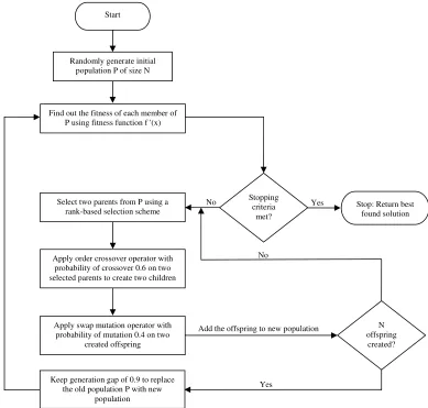
Flow chart of Genetic Algorithm for solving the machine layout problem in cellular manufacturing is shown in Fig. 1. For implementing this model, the following basic components of Genetic Algorithm are considered.

[a] Representation of chromosomes [b] Initial population

[c] Fitness function

[d] Reproduction (Selection) operator

[e] Genetic operators (crossover and mutation) [f] Stopping criteria

[g] Parameters of Genetic Algorithm

A. Representation of Chromosomes

Permutation encoding is used in representing a chromosome. In permutation encoding, each chromosome represents a possible solution such that the length of a chromosome is equal to the number of machines considered in the problem. Individual machine number is represented as a gene in the chromosome. Position of the gene in the chromosome indicates the position of the machine present at that machine location zone.

Example of the chromosome: 6 1 5 8 7 9 2 4 3

In the above example, the length of the chromosome is 9 that are equal to the number of machines considered in the problem. Integer values from 1 to 9 represent the machine number. In the machine location zone, position of machine number 5 is 3.

B. Initial Population

(3)

[image:3.612.135.524.61.432.2]

Figure 1. Flow chart of Proposed Genetic Algorithm

[a] No two or more gene value in the chromosome indicates the same machine number.

[b] The length of the chromosome that is the number of machines is equal to the number of machine location zones.

C. Fitness Function

The process of evaluating the fitness of a chromosome consists of the following two steps.

[a] Evaluate the objective function for each chromosome. [b] Convert the value of objective function of each

chromosome into fitness by using following fitness function equation.

f '(x) = 1/ (1+f(x))

In the above equation, f '(x) is the fitness function of each chromosome and f(x) is the objective function of each chromosome.

D. Reproduction Operator

Several methods exist to achieve this task. The Roulette wheel selection causes the premature convergence and Genetic Algorithm is not able to find out the global optimum solution. In this research work, to find out the global optimum solution rank-based selection is used which does

not suffer from premature convergence. The probability of the ith-selected string is

In the above equation, f ''(i) and f ''(j) is the ranked fitness of the chromosomes i and j respectively.

The algorithm for the rank-based selection process is as follows:

Input: The Population P (N).

Output: The Population after rank-based selection P '' (N). Procedure: Rank_Selection (J1,…………., JN ) :

J’ ←_{sorted population J according fitness with worst} individual at the first position.

S0 ←₀ for i ←_{1 to N}

Si ←_{Si-1 + Pi} end

for i ←_{1 to N}

r ←_{random[ 0, SN ]}

J’’i ←_{J’k such that Sk-1}≤_{r < Sk} end

return { J’’1,………,J’’N } Add the offspring to new population

Start

Randomly generate initial population P of size N

Find out the fitness of each member of P using fitness function f '(x)

Select two parents from P using a rank-based selection scheme

Apply order crossover operator with probability of crossover 0.6 on two selected parents to create two children

Apply swap mutation operator with probability of mutation 0.4 on two

created offspring

Keep generation gap of 0.9 to replace the old population P with new

population

Yes

Yes No No Stopping

criteria met?

N offspring

created? Stop: Return best

(4)

E. Crossover Operator

When Single-point crossover, two-point crossover and uniform crossover are applied to this permutation representation, they are likely to generate infeasible solutions. For example, applying the crossover operator at position 3 creates two infeasible offspring, as illustrated in Fig. 2.

Parent1 (379125486): 3 7 9 | 1 2 5 4 8 6 Parent2 (679813254): 6 7 9 | 8 1 3 2 5 4 ______________________________________________ Offspring 1: 3 7 9 8 1 3 2 5 4 Offspring 2: 6 7 9 1 2 5 4 8 6

Figure 2.Application of the one-point crossover on two parents

So order crossover is used for solving machine layout problem. Order crossover creates offspring by selecting a substring of machines from one parent. It also preserves the relative ordering of machines from the other parent. In order to create an offspring, first copy the string from the first parent between the first crossover point and second crossover point to the offspring and then fill the remaining positions of the offspring by considering the string of machines from the second parent, starting after the second crossover point.

As shown in Fig. 3, in step 1 the substring 125 from parent 1 is copied to the offspring. In step 2 the remaining positions are filled one by one after the second crossover point, by considering the corresponding string of machines from parent 2, as 254679813. Machine 2 is first considered to occupy position 7, but it is discarded because it is already present at position 5 in the offspring. Machine 5 is the next machine to be considered, and it is also discarded. Then, machine 4 is inserted at position 7, machine 6 is inserted at position 8, machine 7 is inserted at position 9, machine 9 is inserted at position 1, machine 8 is inserted at position 2, machine 1 is discarded and machine 3 is inserted at position 3.

parent 1 : 3 7 9 | 1 2 5 | 4 8 6 parent 2 : 6 7 9 | 8 1 3 | 2 5 4 ________________________________________________ offspring

[image:4.612.57.282.454.539.2]

step 1 : - - - 1 2 5 - - - step 2 : 9 8 3 1 2 5 4 6 7

Figure 3.The order crossover

F. Mutation Operator

Again Normal mutation operators generate inadmissible solutions e.g. bit-wise mutation. Let gene i have value x and changing to some other value y would mean that y occurred twice and x no longer occurred.

Swap Mutation for Permutations

[a] Randomly select two machines and swap their positions.

[b] Fig. 4 shows the swap mutation applied on the offspring at position 2 and 7 would generate new mutated offspring.

Offspring : 9 8 3 1 2 5 4 6 7 New mutated offspring : 9 4 3 1 2 5 8 6 7

Figure 4.Swap Mutation

G. Stopping Criteria

When the Genetic Algorithm converges or when it has completed the required number of generations the Genetic Algorithm terminates and displays the machine layout configuration associated with the chromosome with the highest fitness.

H. Parameters of Genetic Algorithm

Genetic Algorithm depends on some parameters like population size, maximum generation number, probability of crossover, probability of mutation and generation gap. Bigger population is better for algorithm’s convergence, because of availability of more genetic material for reproduction, crossover and mutation operators. Changes to build better chromosomes are more. On the other hand, one important issue is algorithm’s speed. Bigger population means more evaluation. Every chromosome in population has to be evaluated in terms of fitness. Usually this procedure is computationally more expensive in Genetic Algorithm. Therefore taking the problem complexity into consideration, population size is kept as 40 and maximum generation number is kept as 100. Again according to genetics, it is obvious that the probability of crossover is always greater than that of mutation. Generally, the probabilities of crossover and mutation are taken as 0.5 to 1 and 0.001 to 0.5 respectively. In this work the probabilities of crossover and mutation are taken as 0.6 and 0.4 respectively. The generation gap is taken as 0.9 which means that at each generation preserving 10% best found solution from old population and other 90% solution from old population is replaced with 90% best found solution from the new population.

V. NUMERICALEXAMPLESANDCOMPARISONOF

ACCURACY

[image:4.612.323.554.545.723.2]

To compare the accuracy of various techniques to solve machine layout problem, input data sets of machine layout problem are taken from Yaman [4]. According to the data sets, 5 parts are processed by 9 machines. Machine location zone is considered as 3X3 grid where earlier researchers have assigned the machines. The input data about the operational sequence and quantitative demands for a five period planning horizon are given in Table 1 and Table 2. The transportation cost per unit is taken as 10.

Table I. Operational sequence of five parts Types of Parts Operation sequence of parts

1 1-3-5-7-2-7-9

2 1-4-2-5-6-8-9

3 1-5-7-8-5-6-2-9

4 1-2-4-6-7-8-2-3-9

5 1-7-6-4-2-8-3-5-6-9

Table II. Quantitative demands of five parts Period

Types of Parts

Period 1 Period 2 Period 3 Period 4 Period 5

1 10 35 90 40 55

2 30 50 25 65 20

3 45 15 40 70 15

4 70 80 55 90 85

(5)

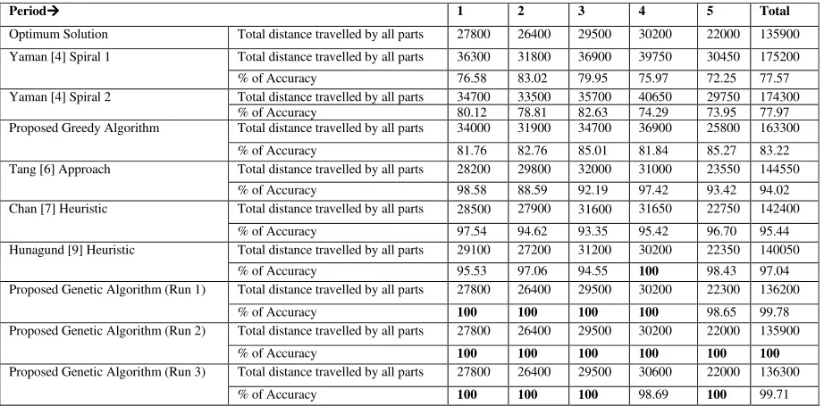
The layout of machines generated and total distance travelled by all parts (objective function value) for each period found by Greedy Algorithm is shown in Fig. 5. For period 2 Greedy algorithm finds out the two solutions with the same objective function value, first solution when 8 is considered as a starting machine and second when 1 is considered as a starting machine. Three runs of Genetic Algorithm are considered. Corresponding to Run 1, 2 and 3, the layout of machines generated and total distance travelled by all parts (objective function value) for each period found by Genetic Algorithm is shown in Fig. 6, Fig. 7 and Fig 8 respectively. From result it is clear that for each period Genetic Algorithm may find out the same solutions (Period 2) or different solutions (Period 5) during the different runs. Again for each run it may find out one solution (Run 3,

Period 3) or multiple different solutions (Run3, Period 1). Accuracy comparison of various techniques to solve machine layout problem is shown in Table 3. Accuracy of various techniques is calculated by comparing the solution generated by various techniques with the optimum solution which can be obtained by either Exhaustive search or Branch-and-bound technique. From the Table 3 it is clear that Genetic Algorithm (Run 2) is able to find out the 100% accurate solution. Also Accuracy of Genetic Algorithm is better than other techniques except for period 4 and Run3. Furthermore compared to other techniques Genetic Algorithm is able to find out the multiple optimum solutions. Multiple solutions are very useful to satisfy the soft constraints of the machine layout problem. For example, as shown in Fig. 7 in Run 2, period 3 Genetic Algorithm finds

Figure 5. Layout of machines generated and total distance travelled by all parts for each period found by Greedy Algorithm Period 2: total

distance travelled 31900 Period 1: total

distance travelled 34000 8

6 5 3

9 7 1

4 2

Period 2: total distance travelled

31900 8

6 7 1

3 5 9

4

2 1

6 7 8

3 5 9

4 2

34700 5

7 2 4

6 7

9 8

1 3

36900 6

8 2 4

1 3 9

7 5

25800 1

6 7 8

3 5 9

4 2

Figure 6. Layout of machines generated and total distance travelled by all parts for each period found by Genetic Algorithm (Run 1) Period 1: total

5 7 6

3 8 9

4 2

26400 4

2 7 8

1 5 3

9 6

29500 9

8 7 2

3 5 1

4 6

30200 6

4 2 8

1 3 9

7 5

22300 4

2 8 7

1 3 9

6 5

8 7 2

9 6 4

1 5

26400 4

2 7 8

1 5 3

9 6

29500 9

8 7 2

3 5 1

4

6 6

4 2 8

1 3 9

7 5

22000 1

2 7 8

4 6

3 9 3 5

29500 1

5 7 6

3 8 9

4 2

2 7 8

4 6 9

3 5

27800 3

8 7 2

9 6 4

1 5

26400 4

2 7 8

1 5 3

9

6 4

2 5 8

1 3 9

7 6

22000 4

6 7 5

9 8

3 3

1 2

29500 9

8 7 2

3 5 1

[image:5.612.55.557.202.734.2] [image:5.612.68.553.225.333.2]

(6)

[image:6.612.77.538.79.311.2]

Table III. Accuracy comparison of various techniques to solve machine layout problem

out the two optimum solutions first solution which assigns the machine 9 to the machine location zone 1 and the machine 1 to the machine location zone 9 while the other solution assigns the machine 1 to the machine location zone 1 and the machine 9 to the machine location zone 9. Now soft constraint may be stated as machine 1 needs to be assigned at machine location zone 1 because of special needs to electricity. Solution 1 does not satisfy the soft constraint and adds extra penalty to the cost of the layout but the solution 2 satisfy it and adds no extra penalty to the cost of the layout. Therefore the multiple solutions generated by Genetic Algorithm have more changes to satisfy the soft constraints of the machine layout problem and thus add no extra penalty to the cost of the machine layout compared to the single solution generated by any other techniques.

If number of machines increases beyond 9 then also Genetic Algorithm, Greedy Algorithm and Hunagund [9] heuristic can be able to solve the layout problem while all other techniques can be applied when the number of machines considered in the problem is less than or equal to nine [9].

VI. CONCLUSION

In this research paper, accuracy comparison of various techniques to solve the machine layout problem is presented. Result shows that Genetic Algorithm is able to find out the 100% accurate solution of the machine layout problem in a reasonable amount of computational time. Comparison shows that Genetic Algorithm outperforms all other techniques in terms of finding the more accurate solutions except for period 4 and Run 3. Genetic Algorithm is able to find out the multiple optimum solutions. Other techniques compared to Genetic Algorithm with no capability of finding out the multiples solutions of the problem have fewer changes to satisfy the soft constraints of the machine layout problem and thus add extra penalty to the cost of the machine layout.

VII. REFERENCES

[1] Tanchoco.J.M.A. and Lee.A.C, “Cellular machine layout based on the Segmented Flow Topology”, International Journal of Production Research, vol. 37(5), 1999, pp.1041–1062.

[2] Bazargan-Lari.M., “Layout designs in cellular manufacturing”, European Journal of Operational Research, vol. 112, 1999, pp. 258-272

[3] K. k. Krishnan, A. A. Jaafari, M. Abolhasanpour and H. Hojabri, “A mixed integer programming formulation for multifloor layout”, African Journal of Business Management, vol. 3(10), Oct. 2009, pp.616-620 [4] Yaman.R, Gethin.D.T. and Clarke.M.J., “An effective

sorting method for facility layout constructions”, International Journal of Production Research, vol. 31(2), 1993, pp. 413-427.

[5] S.P. Singh, “Solving Facility Layout Problem : Three-level Tabu Search Metaheuristic Approach”, International Journal of Recent Trends in Engineering, vol. 1(1), May 2009, pp. 73-77.

[6] Tang.C. and Abdel-Malek.L.L., “A frame work for hierarchical interactive generation of cellular layout”, International Journal of Production Research, vol. 34(8), 1996, pp. 2133-2162.

[7] Chan.W.M., Chan.C.Y. and Ip.W.H., “A heuristic algorithm for machine assignment in cellular layout”, Computers & industrial Engineering, vol. 44, 2002, pp. 49-73.

[8] David E. Goldberg, “Genetic Algorithms in Search, Otimization & Machine Learning”, Pearson Education, 2009.

[9] I.B. Hunagund, and M. Pillai V, “Development of a heuristic for layout formation and design of robust layout under dynamic demand”, Proceedings of the International Conference on Digital Factory, ICDF 2008, August 11-13, 2008 Organized, pp. 1398-1405. [10] Kamaldeep and P. K. Sing, “Multi-Period Planning in

Cellular Manufacturing : A Discussion”, International Journal of Engineering Studies, vol. 2(3), 2010, pp. 251-262.

Period 1 2 3 4 5 Total

Optimum Solution Total distance travelled by all parts 27800 26400 29500 30200 22000 135900

Yaman [4] Spiral 1 Total distance travelled by all parts 36300 31800 36900 39750 30450 175200

% of Accuracy 76.58 83.02 79.95 75.97 72.25 77.57

Yaman [4] Spiral 2 Total distance travelled by all parts 34700 33500 35700 40650 29750 174300

% of Accuracy 80.12 78.81 82.63 74.29 73.95 77.97

Proposed Greedy Algorithm Total distance travelled by all parts 34000 31900 34700 36900 25800 163300

% of Accuracy 81.76 82.76 85.01 81.84 85.27 83.22

Tang [6] Approach Total distance travelled by all parts 28200 29800 32000 31000 23550 144550

% of Accuracy 98.58 88.59 92.19 97.42 93.42 94.02

Chan [7] Heuristic Total distance travelled by all parts 28500 27900 31600 31650 22750 142400

% of Accuracy 97.54 94.62 93.35 95.42 96.70 95.44

Hunagund [9] Heuristic Total distance travelled by all parts 29100 27200 31200 30200 22350 140050

% of Accuracy 95.53 97.06 94.55 100 98.43 97.04

Proposed Genetic Algorithm (Run 1) Total distance travelled by all parts 27800 26400 29500 30200 22300 136200

% of Accuracy 100 100 100 100 98.65 99.78

% of Accuracy 100 100 100 100 100 100