Infective Susceptible Phase Plane Analysis in the Extended SIR Model I

Volume 3, No. 7, Nov-Dec 2012

International Journal of Advanced Research in Computer Science

RESEARCH PAPER

Available Online at www.ijarcs.info

ISSN No. 0976-5697

Infective Susceptible Phase Plane Analysis in the Extended SIR Model-I

N Suresh Rao

Department of Computer Centre / Computer Science and IT Block University of Jammu Jammu- J & K State, India

suresh_jmu@yahoo.co.in

Abstract: In the present investigation an attempt is made to understand the I-S phase plane. Trajectories, using the solutions of the second order differential equation, describing the virus growth in the extended model of SIR covering immigration studies, are presented. The value of the ratio of product of immigrant rate and birth rate of virus to square of death rate of virus, greater than or equal to value four, plays a dominant role in deciding the nature of I-S trajectories. For same values of immigration rate, birth and death rates of virus the trajectories reach asymptotically the stable equilibrium point (ratio of death and birth rate of virus, ratio of immigration and death rate of virus) which is termed as a nodal sink. Effect of low and high values of death rate, birth rate and threshold value along with different population sizes is also illustrated therein.

Keywords: Immigration, SIR model, I-S phase plane, Virus Growth, Birth and death Rates, 2nd Order Differential equations.

I. INTRODUCTION

The concept of immigrants plays an important role in the field of demographic studies. The inflow of population has a tremendous impact on the socio-economic-environmental values on the existing conditions in a given population. Similarly in the study of epidemics, immigrants play a vital role. This can be understood by transmission of virus leading to new class of diseases e.g., HIV leading to AIDS [1]. It is needless to emphasize in the field of computers also, in view of similarities between computers and biological viruses, the immigrants (the influx of computers) play an important role on the growth and spread of virus. To carry out such studies, SIR (susceptible- infected-removed) model [2] is convenient when extended to the inclusion of immigrants at a constant rate in the prevailing system of computers. Such studies have been made in [3], [4]. In these studies the attention was paid mostly for the general understanding of spread and growth of virus in computers.

The particular study of infected susceptible phase plane analysis throws lot of light on the relative removal rate, basic reproduction rate, birth and cure rates of computer virus [5].The theoretical implications of the analysis was explained in Appendix-I [6]. A simple and elegant method of solving the second order differential equation for the virus growth was given by extended model of SIR [7], where in one of the solutions leading to complex roots for the virus growth was dealt. Out of the other two solutions, where the roots are (i), real and distinct and (ii), real and equal, the situation (i) real and distinct roots is presented in this publication while the situation (ii) real and equal roots is going to appear in a forth coming publication. The subject matter is arranged as follows. In section II the methodology is described. In section III the results and discussions are presented where as in section IV, the conclusions are high lighted. Finally, references are given in section V.

II. METHODOLOGY

The basic SIR model involves three classes of systems namely susceptibles(S), infectives (I) and removed(R). Some susceptibles (immigrants) at a constant rate (k) into the system are introduced. Thus, the effect of immigrants on the spread and growth of virus was discussed in detail by [7]. The prominent equations governing the virus growth are given by:-

SI

With the condition,

kt

Where k stands for immigrant rate, β for birth rate, γ for

death rate, S0, I0 are initial values of S and I. N stands for

population size. It may be noted that all the three derivatives in “(1)” cannot vanish simultaneously. We confine our

discussion to the first two derivatives. Let SE and IE

correspond to equilibrium solution. By setting the first two derivatives in “(1)” = 0 one can obtain the steady

state/equilibrium solutions SE and IE. In general the values of

S and I can be expressed in terms of SE and IE by introducing

small departures ε and υ respectively. The values of ε and υ

are so small so that their squares, higher powers, and product terms can be neglected. On substituting in “(1)” and simplifying, one can obtain relations amongst ε, υ,

dt

dε _{, and}

dt

dυ_{. In these relations with suitable substitution and}

simplification one can eliminate ε. This exercise will result in

a second order differential equation in υ as

υ'' ₊( β γ)υ'₊( β)υ₌0

k

k (3)

This can be solved by standard method. In doing so one comes across a discriminator

ω = 1 4*(_kβ γ)2 −_kβ) ₍₄₎

The valu e of ω may b e +ve, zero or –ve according to

k respectively. Accordingly the roots are (i)

real and distinct, (ii) real and equal, (iii) complex and unequal.

A. Roots are real and distinct:

In general the solution is given by

c

,

c

₂ are arbitrary constants which can be derived from

initial conditions. Values of υ and υ’

thereby I are found as a function of time. Similarly the

expressions, ε= (1/γ)*υ,S=SE(1+ε) whereSE =γ/β, the

equilibrium value ofS, are used to determine the values of ε

and there by S as a function of time. One can also plot

I

vs

S

for different combinations ofK, β and γ preserving the

condition that

β

/

γ

2 > 4

k .

III. RESULTS AND DISCUSSIONS

In the present investigation the main interest is focused on

the I_S phase plane analysis. Thus out of the three coupled

differential equations used, the first two are sufficient for discussion. Unlike SIR model, the

dt

dS _{equation is not a}

continuously decreasing function. It has no lower bound limit.

On the contrary it has i) a term,−βSI, representing the

number of susceptibles getting converted into infectives and

ii) a term, K , representing an inflow of immigrants at a

constant rate. So depending on the initial values of

S

,

I

,β

and K , there will be a competition between the said two

terms. As a result

dt

dS will be increasing / decreasing. In the

second equation,

dt

dI _{will be +ve, 0, -ve asS>,=,<γ/β. The}

value of γ/β is termed as threshold value or effective removal

rate (

ρ

). Thus increase/decrease of

I

with time depends on

whether S >

ρ

orS < ρ . It may be noted that at

equilibrium state the two differential equations,

dt

B. Roots are real and distinct:

According to the above prescriptions of the model different

values of parameters, N , I₀, K,

γ

, β of the virus are

chosen so that conditions needed for Sec: II-A are satisfied.

Further two sets of values for (i) high

γ

,

β

and low

ρ

and

(ii) low

γ

, β and high

ρ

are considered. Obtain S and I, as

a function of time. With appropriate choice of input

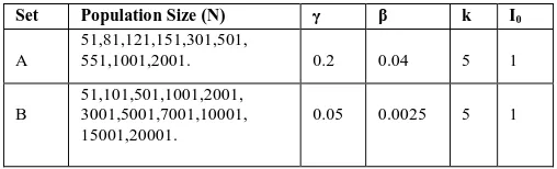
parameters the effect of different values of γ (0.2 to 0 .05) and

β (0.04 to 0.0025) or in other words different values of ρ (5 to 20) and various population sizes (N=51 to 20,001) is studied,

with respect to the virus growth and time taken to reach SE &

IE, through numerical simulations. Out of the figures drawn

and studied exhaustively, for I vs S; S vs t and I vs t, two typical sets of data (A and B) as mentioned are considered. The relevant data is shown in Table 1 and the results are described below.

Table 1: Input parameters data

Set Population Size (N) γ β k I0

While studying the, I vs S trajectories some distinct

features are noted irrespective of γ and β, accordingl y, they are

classified into three different phases.

Phase I: In this phase the values of S increase from S0 up

to a maximum value. The trajectory takes a reversal i.e. S

decreases and finally reaches the value SE asymptotically. The

value of S is > SE. Thus I will be increasing from I0 to IE

asymptotically.

Phase II: In this case S will be decreasing from the

beginning i.e. S0 and asymptotically attains the value SE .Here

again the value of S is > SE i.e. ρ. Thus I will be increasing

from I0 to IE asymptotically.

Phase III: In this phase also S will be decreasing from S0,

passes through SE and enters –ve region for a while and then

with a reversal enters +ve region and finally attains SE and

continues to remain there for all the times. It may be noted that

the value of S, till it passes the ordinate at SE, will be > SE and

later on the value will be < SE till it sinks to the value SE. For

this region S will be < ρ. Thus I will increase to a maximum value and then will decrease exponentially and asymptotically

attains the equilibrium value IE. This feature is in accordance

with the second differential equation of (1).

For clarity in resolution, the I vs S trajectories are shown in “Figs.1.1.1, 1.1.2 and 1.1.3” for N=51, 81,121; 151,301,501; 551, 1001, 2001 respectively in set A. These three diagrams represent the three phases of I vs S trajectories as explained already. Similarly I vs t is shown in “Fig 1.2” for selected values of N =81, 301, 551, 1001. The variation of S vs t for N=81,301 is shown in “Fig. 1.3.1” and for N=551, 1001 is shown in “Fig. 1.3.2”. The features exhibited in all the graphs are in accordance with the prescription of the model.

From the numerical values obtained for I and S as a

function of time, it is noted that the time taken to attain IE and

SE values is close to 50 unit time steps. Further the value of IE

is reached earlier compared to the value SE. In order to have a

feeling about the effect of low γ and β values, ρ is increased

0

-200 400 1000 1600

Susceptibles ( S )

Series1 Series2 Series3 Series4

Series 1 : N = 81 Series 2 : N = 301 Series 3 : N = 551 Series 4 : N = 1001

0

0 500 1000 1500 2000 2500

Susceptible ( S )

I

Series1 Series2 Series3 Series4 Series5

Series 1 : N = 51

0 1000 2000 3000 4000 5000 6000 7000 8000

Susceptible ( S )

0

-2000 2000 6000 10000 14000 18000

Susceptibles ( S )

Series1 Series2 Series3 Series4

Accordingly all the drawings for I vs S for N=51,101,501,1001,2001;3001,5001,7001;,10,001,15,001,20, 001, I vs t for N=501,5001,10,001,15,001 and S vs t for N=501,5001;10,001,15,001 for set B are shown in “Figs.2.1.1, 2.1.2, 2.1.3; 2.2 and 2.3.1, 2.3.2” respectively. All the features as exhibited in “Fig.1” series are noted in “Figs. 2” series also. The corresponding population sizes at the transition of phases are enhanced e.g. for set A, the value of N is less than 121 for phase-I, lies between 151 to 501 for phase-II and greater than 551 for phase-III. Where as for the set B, the corresponding values are less than 2001 for Phase-I: for Phase-II limits are 3001 to 7001 and for phase-III the value is greater than 7001. Similarly the time taken to attain the equilibrium values for I and S is also enhanced to nearly 200 unit time steps. Again it is observed, that I attains the equilibrium value prior to that of

S. Thus on comparing the results from set A to set B i.e. ρ

from lower to higher value, one comes across higher values for population sizes and also time taken to reach equilibrium values for I and S. It can be verified that when ρ is increased by a factor of 4, the saturation times also increased by a

similar factor. Thus it may be noted that higher the value of ρ

slower is the growth of virus.

IV. CONCLUSIONS

In this investigation the term

k

β

/

γ

2 plays an important

role in describing the nature of infection growth. Unlike SIR model there is no lower bound to S but it attains a stable

equilibrium value, SE = ρ, which is the th reshold valu e The

Increasing / decreasing trend of

S

depends on the relative

strengths of the terms,

−

β

SI

, k. The

I

value will not tend to

zero but attains a stable equilibrium value for

I

E

=

k

/

γ

.

Variation of I depends on whether S >ρorS ≤

ρ

. For

same values of k, γ and

β

, all trajectories in

I

_

S

phase

plane reach the stable equilibrium point at (

S

_E

,

I

_E) which is

termed as nodal sink. It is observed that as the threshold value

is increased, the time taken to reach equilibrium point (SE,IE)

also increases indicating there by the slow rate for growth of virus.

V. REFERENCES

[1]. H. J. Kim, “The continuous model for the transmission of HIV”, Research Project, Univ of Washington.2008.

[2]. N. Suresh Rao, Devanand, P.S. Avadhani.,“Propagation behavior of computer virus in the frame work of SIR model”, Journal of Comp.Sc, ICFAI, Vol .III, No 4, pp 1-11.,2009.

[3]. E. Shim, “An epidemic model with immigration of infectives and vaccination”, M.S.Thesis, Univ of British Coulombia.,2002.

[4]. T.W.Huang, “A Mathematical model for infectious diseases-an extended SIR model”, Research Project, National Univ. Kaohsiung, Taiwan-811, R.O.C. ,2008.

[5]. E.A Allaman and J.A. Rhodes., “Mathematical models in Biology: An Introduction” , Cambridge Univ Press, 2004.

[6]. J.D. Murray., “Mathematical Biology”, Springer-Verlag,3rd Edn, New York.,2002.