Data Mining Techniques for Efficient Detection of Cancerous Masses in Mammogram

Volume 3, No. 1, Jan-Feb 2012

International Journal of Advanced Research in Computer Science

RESEARCH PAPER

Available Online at www.ijarcs.info

ISSN No. 0976-5697

Data Mining Techniques for Efficient Detection of Cancerous Masses in Mammogram

S.Pitchumani Angayarkanni* M.C.A.,M.Phil(Ph.D)

Assistant Professor,Department of Computer Science, Lady Doak College,Madurai, India

[email protected]

Dr.Nadira Banu Kamal H.O.D,Department of M.C.A,

TBAK College, Kilakarai, India [email protected]

Abstract: Breast cancer is the most common form of cancer in women. Early diagnosis of cancerous masses and its size for treatment can prolong the life time of the patients. An intelligent computer-aided diagnosis system can be very helpful for radiologist in detecting and diagnosing micro calcifications patterns earlier and faster than typical screening programs. A number of quantitative models including linear discriminate analysis, logistic regression, k nearest neighbor, kernel density, recursive partitioning, and neural networks are being used in medical diagnostic support systems to assist human decision-makers in disease diagnosis. This research mainly focuses on the decision accuracy of online Back Propagation Neural network model with data mining technique for the diagnosis of cancerous masses from the non cancerous region with accuracy and speed. Conditions where a hierarchical neural network model can increase diagnos tic accuracy by partitioning the decision domain into subtasks that are easier to learn are specifically addressed in this paper through decision tree inducti on method. Self-organizing maps (SOM) are used to portray the 9 feature variables in a two dimensional plot that maintains topological ordering. The SOM identifies five inconsistent cases that are likely sources of error for the quantitative decision models; the lower bound for the diagnostic decision error based on five errors is 0.266. The traditional application of the quantitative models cited above results in diagnostic error levels substantially greater than this target level. A multilayered feed forward neural network is designed for detect. The second stage mixture-of-experts neural network learns a subtask of the automatic detection of diagnostic decision, the discrimination between benign, malignant and normal cases. The diagnostic accuracy of the multilayered feedforward neural network approaches the target performance established from the SOM with an error rate of 0.0012 and accuracy of 99.9%.

Keywords: Preprocessing, Gabor Filter, Decision Tree Induction, SOM and ANN

I. INTRODUCTION

Breast cancer is one of the major causes for the increase in mortality among women. A tumor is a mass of tissue that grows out of the normal faces that regulate growth. Early diagnosis requires accurate and reliable diagnosis procedure that allows the physicians to distinguish benign from malignant without going for surgical biopsy. The prediction must classify the patients to either benign or malignant.

Many different algorithms have been proposed for automatic detection of breast cancer in mammograms. Feature extracted from mammogram images can be used for detection of cancer. Many proposed algorithm did not analyze the texture component of the image in detail. The proposed algorithm performs classification based on the analysis of the nine texture parameters; further Knowledge Discovery Database KDD which includes Data Mining technique is incorporated to generate test cases for the two layered ANN. The logic of Decision Tree is very easy to discern. The proposed algorithm produces an accuracy of 99.99% with a minimum error rate of 0.001%.The main objective of this paper is to develop a CAD system for automatic detection of breast cancer through MRI. The proposed system can provide the valuable outlook and accuracy. Of earlier breast cancer detection. It consists of five stages .

a.Preprocessing and enhancement

b.Feature extraction, selection and classification c.Segmentation of suspicious region

d.Deriving the decision rule and formulating decision tree.

e.Automatic segmentation using two layered ANN.

II. DATABASE

The MIAS database which contains left and right breast images of 190 records. It consists of 285 images which belongs to three types as Normal, Benign and Malignant. There are 200 normal, 50 benign and 35 malignant images.

III. PREPROCESSING AND ENHANCEMENT

The preprocessing stage is used for reducing image noise, highlighting edges or displaying digital images. The enhancement stage includes resolution and contrast enhancement. They are used mainly to suppress noise and imaging of spectral parameters. It Converts the Medical image into standard image without noise, film artifacts and labels.

A. Preprocessing:

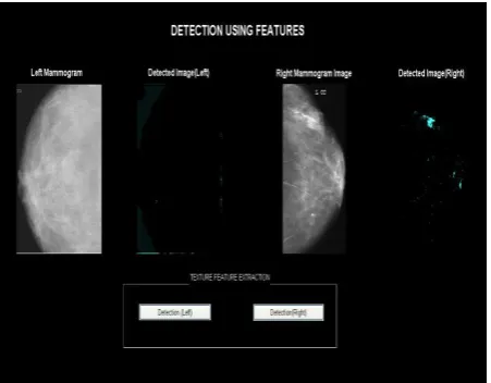
Preprocessing indicates that the same tissue type may have a different scale of signal intensities for different images. Preprocessing function involve those operations that are normally require prior to the main data analysis and extraction of information .The texture based technique with histogram equalization is applied to the left and right MRI mammogram images. This shows detections of tumor with decrease in pixel count in binary images, increase in image intensity. High numbers of high intensity pixels. Remove pectoral muscles which help in predicting the tumor more accurately.

B. Enhancement:

extracted. It extracts the edge of the tumor from surrounding normal tissue and background.

Figure 1: Preprocessing and Enhancement

IV. TEXTURE ANALYSIS

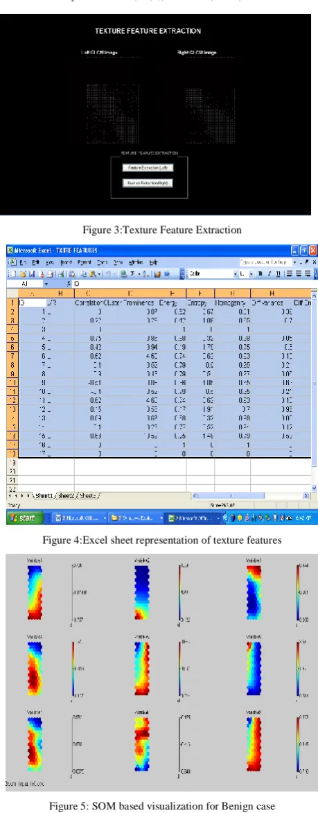
Texture based segmentation is implemented because when a person is affected by cancer the texture of the skin becomes smooth.This Segmentation method segments the calcification pattern and the other suspicious regions in the mammograms. Using GLCM (Gray level co-occurrence matrix) technique we how often different combination of brightness values occur in an image. The GLCM image is divided into 3x3 matrix and the texture features are calculated. Texture Features are: Cluster Prominence, Energy, Entropy, Homogenity, Difference variance, Difference Entropy, Information Measure, Normalized, correlation

V. TEXTURE FEATURE ANALYSIS–(SELF

ORGANIZATION MAP)

a. A self-organized map (SOM)-type of artificial neural network that is trained using unsupervised learning to produce a two-dimensional, representation of the training samples, called a map(Kohonen Map).SOM operate in two modes: Training and Mapping. Training builds the map using input samples(vector quantization). Mapping automatically classifies a new input vector.The map constitutes of neurons/node located on a regular map grid. The lattice of the grid can be either hexagonal or rectangular.

Figure 2: Training

The blue blob is the distribution of the training data, and the small white disc is the current training sample drawn from that distribution. The map constitutes of neurons/node located on a regular map grid. The lattice of the grid can be either hexagonal or rectangular.The SOM Toolbox is designed to perform the Training and Mapping functions .We find which Texture Feature is used for detecting tumor in the mammograms. By analyzing different cases of Mammograms we find that only Variable 8 (Information Measure) differs.

Figure 3:Texture Feature Extraction

Figure 4:Excel sheet representation of texture features

Figure 5: SOM based visualization for Benign case

VI. WATERSHED SEGMENTATION

a. The Detected Region can be segmented using Watershed Segmentation

b. Watershed transition form usually works well only with images of bubbles or metallographic pictures, but when combined with filter techniques, it works well. c. The detected image is superimposed with the original

Figure 6: Segmentation of LEFT Image – Benign case

VII. ASSOCIATION RULE MINING USING

APRIORI ALGORITHM:

It is mainly used to search for interesting relationships among items in a given data set.

Algorithm:

Apriori:Find frequent itemsets using an iterative level-wise approach based on candidate generation.

Input: Excel file of Texture parameters D; minimum support threshold, min_sup

Output:L, frequent itemsets in D. Method:

Pass 1

a. Generate the candidate itemsets in C1

b. Save the frequent itemsets in L1 Pass k

a. Generate the candidate itemsets in Ck from the

frequent itemsets in Lk-1

a. Join Lk-1 p with Lk-1q, as follows:

insert into Ck

select p.item1, p.item2, . . . , p.itemk-1, q.itemk-1

from Lk-1 p, Lk-1q

where p.item1 = q.item1, . . . p.itemk-2 = q.itemk-2, p.itemk-1 < q.itemk-1

b. Generate all (k-1)-subsets from the candidate itemsets in Ck

c. Prune all candidate itemsets from Ck where some

(k-1)-subset of the candidate itemset is not in the frequent itemset Lk-1

d. Scan the transaction database to determine the support for each candidate itemset in Ck

e. Save the frequent itemsets in Lk

VIII. DECISION TREE INDUCTION METHOD,

J48 ALGORITHM:

The J48 Decision tree classifier follows the following simple algorithm. In order to classify a new item, it first needs to create a decision tree based on the attribute values of the available training data. So, whenever it encounters a set of items (training set) it identifies the attribute that discriminates the various instances most clearly. This feature that is able to tell us most about the data instances so that we can classify them the best is said to have the highest information gain. Now, among the possible values of this

feature, if there is any value for which there is no ambiguity, that is, for which the data instances falling within its category have the same value for the target variable, then we terminate that branch and assign to it the target value that we have obtained.

For the other cases, we then look for another attribute that gives us the highest information gain. Hence we continue in this manner until we either get a clear decision of what combination of attributes gives us a particular target value, or we run out of attributes. In the event that we run out of attributes, or if we cannot get an unambiguous result from the available information, we assign this branch a target value that the majority of the items under this branch possess.Now that we have the decision tree, we follow the order of attribute selection as we have obtained for the tree. By checking all the respective attributes and their values with those seen in the decision tree model, we can assign or predict the target value of this new instance. The above description will be more clear and easier to understand with the help of an example. Hence, let us see an example of J48 decision tree classification.

=== Classifier model (full training set) === J48 pruned tree

--- Node7 = Value1 | Node5 = Value1

| | Node8 = Value1: Value1 (15.0/3.0) | | Node8 = Value2

| | | Node2 = Value1: Value1 (7.0/2.0) | | | Node2 = Value2: Value2 (12.0/2.0) | Node5 = Value2

| | Node8 = Value1: Value2 (15.0) | | Node8 = Value2

| | | Node4 = Value1

| | | | class = Value1: Value2 (3.0/1.0) | | | | class = Value2: Value1 (6.0/1.0) | | | Node4 = Value2: Value2 (6.0/1.0) Node7 = Value2

| Node4 = Value1 | | Node5 = Value1

| | | Node9 = Value1: Value2 (4.0) | | | Node9 = Value2: Value1 (4.0/1.0) | | Node5 = Value2

| | | class = Value1

| | | | Node2 = Value1: Value2 (2.0) | | | | Node2 = Value2: Value1 (3.0/1.0) | | | class = Value2: Value1 (11.0/1.0) | Node4 = Value2: Value1 (12.0/1.0) Number of Leaves: 13 Size of the tree: 25

Time taken to build model: 0.03 seconds Time taken to build model: 0.05 seconds Number of training instances: 100 Number of Rules: 16

Non matches covered by Majority class. Best first.

Start set: no attributes Search direction: forward

Stale search after 5 node expansions Total number of subsets evaluated: 76 Merit of best subset found: 75

Time taken to build model: 0.14 seconds

Figure 7:Dendrogram for Benign and Malignant cases

IX. NEURAL NETWORK CLASSIFICATION

Multilayered feed forward neural network is used for training in this proposed method. Reason for choosing multilayer BPN is that it involves non parametric statistical properties. Unlike the classical statistical classification methods, such as bayes classifier no knowledge of the underlying probability distribution is needed by a neural network. It can learn the free parameters (weight and bias) through training by example. This makes it suitable to deal with real problem which are nonlinear, non stationery and non Gaussian. The neural network classifier is used to generate a likelihood map of each mammogram using gabor feature as input to classifier.

The feature set extracted from 285 gabor feature set classified using the Association rule based Decision tree induction is used to classify benign, malignant and normal cases .These feature sets are given as input to the network for training. The desired output from the network is whether the classification is malignant, benign or normal tissue. Four neurons are used in hidden layer and the nine feature sets are used in input layer. During the training session of the network a pair of pattern is presented, the input pattern and target pattern (Malignant, Benign and Normal). At the output layer, the difference between the actual and target output yields an error signal. This error signal depends on the values of the weights of the neurons in each layer. This error is minimized and during these process new values for the weights obtained.

Data partition results:

190 records to Training set (68.35%) 44 records to Validation set (15.83%) 44 records to Test set (15.83%) Data anomalies:

17 numeric outliers

Architecture selected manually

[9-4-1] architecture selected for training Hidden layers activation function: Logistic Output parameters:

Normalized

Error function: Sum-of-squares Activation function: Logistic

Figure 8: Multilayered BPN

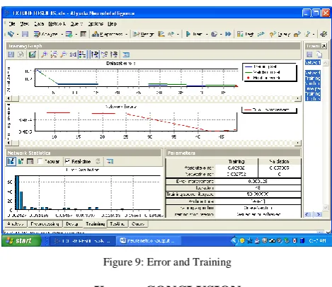
Network architecture: [9-4-1] Training algorithm: Quasi-Newton Number of iterations: 48

Time passed: 00:00:00

Training stop reason: Desired error achieved The best network was tracked and restored

Figure 9: Error and Training

X. CONCLUSION

The proposed algorithm increases the diagnosis rate of cancerous masses in mammogram with minimum error and accuracy of 99.99%. The The rule generated using decision tree induction method clearly shows that the time taken t classify benign and malignant cases in just 0.03 seconds and the accuracy was 99.9%. The specificity =t-neg/neg, sensitivity =t-pos/pos and Precision=t-pos/t-pos+f-pos and accuracy is =sensitivity (pos /(pos+neg)) +specificity (neg/(pos+neg)).

From the above algorithm the accuracy was found to be 99.9%. The proposed method yields very good accuracy in minimum period of time shows the efficiency of the algorithm.

XI. REFERENCES

[2]. Ruchaneewan Susomboon, Daniela Stan Raicu, Jacob Furst.:Pixel – Based Texture Classification of Tissues in computed Tomography.: Literature review (2007)

[3]. De Cock, M.Cornelos, C.Kerre E.E. : Fuzzy Association Rules : A Two – sided Approach In : FIP, PP 385-390(2003)

[4]. H. B. Kekre, Tanuja K. Sarode, Bhakti Raul, “Color Image Segmentation using Kekre’s Algorithm for Vector Quantization”,International Journal of Computer Science(IJCS), Vol. 3, No. 4, pp.: 287-292,Fall2008. Available:http://www.waset.org/ijcs.

[5]. H. B. Kekre, Tanuja K. Sarode, Bhakti Raul, “Color Image Segmentation using Vector Quantization Techniques Based

on Energy Ordering Concept” International Journal of Computing Science and Communication Technologies (IJCSCT) Volume 1, Issue 2, pp:164-171, January 2009.

[6]. Braz Junior, G., Silva, E. C., de Paiva, A. C., Silva, A. C., & Gattass, M. (2007). Breast Tissues Mammograms Images Classification using Moran's Index, Geary's Coefficient and SVM. In: 14th International Conference on Neural Information Processing (ICONIP 2007), 2007, Kitakyushu. Lecture Notes Computer Science--LNCS.