216
A COMPARATIVE STUDY OF DENOISING 1-D
DATA USING WAVELET TRANSFORM
Hemant Tulsani
1, Rashmi Gupta
21 2 Electronics and Communication Department
1 2 Ambedkar Institute Of Advanced Communication Technologies And Research New Delhi-110031, India
ABSTARCT:
In this paper, discrete wavelet transform (DWT) for noise removal has been studied over four different types of synthetic data. These are blocks signal, bumps signal, doppler signal and heavy sine signal. These signal sets are first corrupted with white noise and then DWT is used for noise removal. The impact of different levels of decomposition along with the type of thresholding criterion, hard or soft, over output signal to noise ratio (SNR) and mean square error is presented. The waveforms of original and reconstructed signals for all levels of decomposition is also presented in the paper. All simulations are done in MATLAB.
Keywords: Wavelets based denoising, Signal decomposition, Hard Soft Thresholding
1. INTRODUCTION
Role of signals and systems is important in all aspects of modern technologies. However, a certain amount of unwanted signal i.e., noise is always introduced in digital signals. The noise is generally introduced while acquisition and transmission of data signals.
Introduction of noise in any signal degrades the quality of signal as well as the information content of the signal is lost to some extent. Hence, it is highly necessary to remove noise from the signal so that the information can be recovered from it. This type of signal restoration which is associated with an attempt of removal of noise from a signal is known as denoising. Noise is considered to have higher frequencies compared to signal. Hence, filtering was the most popular technique applied for denoising applications. Different linear and non-linear filters are proposed by researchers. Some examples of filters are mean filter, median filter, least mean square (LMS) filter, wiener filter, etc. Research in this field has led to development of new denoising techniques such as optimal estimate methods, spectral subtraction methods, general and genetic matching pursuit methods. However, the newest approach in this field is denoising using wavelet transform method.
The traditional methods for denoising were based on the Fourier transformation and the short-time Fourier transformation [13] but the analysis effects of them were not good enough as the requirement was time frequency representation of signal. In Fourier transformation, the signal analysis is done completely in frequency domain. It can only analyze what frequency components exist in the signal. Hence, the time and frequency information could not be analyzed at the same time. The concept of short-time Fourier transformation (STFT) analysis is a bit different and comparatively better. It used the concept of windowing the signal i.e., analyzing only a small section of the signal at a time.
217
The discrete wavelet transform and it's variants is based on dyadic decomposition of a input signal into approximation and detail coefficients. Based on the methodology employed in decomposition of signals, wavelet transform may be termed as Discrete Wavelet Transform (DWT) or Discrete Wave Packet Transform (DWPT) [11] [12]. In DWT, only the approximation coefficients at each level are further decomposed. In DWPT, detail coefficients along with approximation coefficients are decomposed. Discrete wavelet transform (DWT) is a powerful tool using multi-resolution analysis (MRA) to analyze a signal. It has been used in speech recognition systems, signal and image compression and denoising.
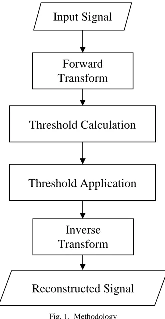
2. METHODOLOGY
The basic methodology is used in noise removal in wavelet domain is shown in Figure 1.
2.1.Forward Transform
Input signal is transformed to wavelet domain using discrete wavelet transform.
2.2.Threshold Calculation
Removal of noise from a signal using wavelets is based on thresholding technique called wavelet thresholding. It is a non-linear technique. In this, some of the wavelet decomposed coefficients particularly detail coefficients which contain noise elements which are less than a predefined or dynamically computed threshold are made zero. Hence, this process is also known as wavelet shrinking [1]. Selecting an appropriate threshold is a topic of utmost importance as the efficiency of the algorithm entirely depend on its selection [2].
Fig. 1. Methodology
Input Signal
Forward
Transform
Threshold Calculation
Threshold Application
Reconstructed Signal
Inverse
218
Global and Level dependent Threshold
The calculation of threshold may or may not depend on the decomposition levels. If a threshold value is selected for each decomposition level , then the threshold is said to be level dependent threshold. However, if a same threshold value is calculated for coefficients at all levels, then the threshold is termed as global threshold [3] [14].
Various functions have been proposed to calculate an appropriate threshold value. Most accepted of those include VisuShrink and SureShrink. These are explained below.
VisuShrink
VisuShrink was introduced by Donoho [6]. It uses a threshold value
t
that is proportional to the standard deviation of the noise. It follows the hard thresholding rule. It is defined as:2 log
t
=
σ
n
. (1)2
σ
is the noise variance present in the signal and represents the signal size or number of samples. An estimate of the noise level was defined based on the median absolute deviation given by:{
}
where
d
j−1,k corresponds to the detail coefficients in the wavelet transform.VisuShrink can be viewed as general-purpose threshold selector which provide near optimal error properties. It also ensures that the estimates are as smooth as the true underlying functions.
Major drawbacks of VisuShrink include overly smoothed reconstructed signals as it removes too many coefficients, only applicable to signal corrupted with AWGN, and following of global thresholding scheme.
SureShrink
A threshold chooser based on Stein’s Unbiased Risk Estimator (SURE) was proposed by Donoho and Johnstone [6] and is called as SureShrink. It is a combination of the universal threshold and the SURE threshold. This method specifies a threshold value for each resolution level in the wavelet transform which is referred to as level dependent thresholding. The goal of SureShrink is to minimize the mean squared error, defined as
(
)
2 length of the signal. SureShrink suppresses noise by thresholding the empirical wavelet coefficients.The SureShrink threshold
t
∗ is defined asmin( ,
2 log )
t
∗=
t
σ
n
. (4)219 2.3.Threshold Application
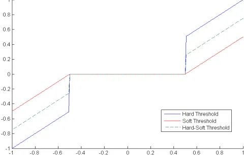
After calculating a threshold value, a thresholding function
f x
( )
is required which is applied to threshold the coefficients. This function is dependent upon the threshold valuet
. There are two general categories to threshold function. They are hard threshold and soft threshold functions [8]. The hard threshold function [7] can be expressed as:The soft threshold function [5] can be expressed as:
( )
Soft Threshold function is known to perform well in smooth regions but it over smooth sharp features. Hence the sharp characteristics of signal are lost.
Therefore, a new threshold function, hard-soft threshold was presented which unifies soft and hard threshold and may retain the chief signal features and at the same time, be possible to meet the smoothness requirements. The expression for hard-soft threshold is given below:
( )
The parameter
α
(scaling factor) defines the boundary between the hard and soft thresholding. Ifα
=
1
, the function follow soft threshold whileα
=
0
follow hard threshold. The choice of 0<α<1 tend to overcome the drawbacks of both hard and soft threshold functions.The different threshold functions are shown in Figure 2. It can be inferred that hard threshold function keeps all
the values of the signal for
x
≥
t
while completely removes all other values. Soft threshold function workssimilar to hard threshold except that it scales down the values. Hard soft threshold function provides a compromise between the other functions.
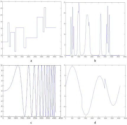
220 3. SIMULATION SETUP
Four simulated signals are used for experimentation purpose. They are corrupted with additive white noise resulting in a noisy signal. Figure 3 show the four signals used, and Figure 4 show the corresponding noisy signals obtained.
a
b
c
d
221
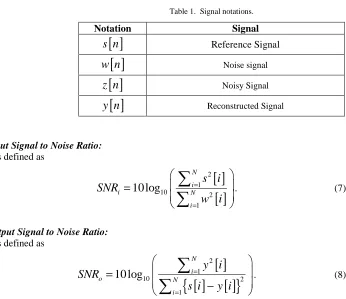
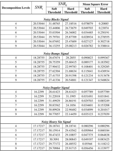
To compare the performance of proposed threshold selection algorithms and wavelet decomposition algorithms for one dimensional data, few parameters [9] [10] have to be computed for each case. The signal notations followed in this text are tabulated in Table 1.
a
b
c
d
222
Input Signal to Noise Ratio:
It is defined as
Output Signal to Noise Ratio:
It is defined as
Mean square error value should be minimum for better algorithm.
The wavelets used for evaluation purposes are haar for blocks and db8 for rest signals. The threshold selector used is universal threshold selector or VisuShrink. Different decomposition levels are also compared for performance evaluation which are 4, 5, 6, 7, 8 and 9. The results for soft and hard thresholding criterion are also compared.
4. RESULTS AND DISCUSSION
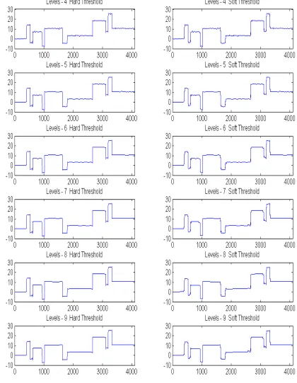
The results are compiled for each signal discussed in previous section one by one. First, the results of denoising noisy Blocks signal, Bumps signal, Doppler signal, Heavy Sine signal for all levels of decomposition are shown in figures 5, 6, 7 and 8.
223
224
225
226
227
6 20.53044 35.03504 26.36002 0.034485 0.250191
7 20.53044 35.79701 25.87709 0.028934 0.278555
8 20.53044 36.07692 25.47609 0.027127 0.302718
9 20.53044 36.13255 25.08213 0.026782 0.330014
Noisy Bumps Signal
4 18.28755 28.67674 28.2855 0.090823 0.099367
5 18.28755 28.75359 25.60415 0.089177 0.183502
6 18.28755 27.90432 22.99783 0.108401 0.329285
7 18.28755 27.62304 21.68634 0.115641 0.436934
8 18.28755 27.41755 20.91398 0.121234 0.513478
9 18.28755 27.41336 20.54881 0.121347 0.548824
Noisy Doppler Signal
4 17.17217 28.18741 28.18741 0.080296 0.080296
5 17.17217 30.15914 29.43562 0.050964 0.060184
6 17.17217 30.47433 29.10857 0.047375 0.064838
7 17.17217 30.3091 28.00843 0.049197 0.083425
8 17.17217 29.77172 26.48552 0.05566 0.118212
9 17.17217 29.70984 25.91715 0.056456 0.133977
Various conclusions can be drawn from the results. The impact of hard and soft threshold functions can be summarized as below:
(1)Soft Thresholding performs well in smooth regions.
(2)Soft Thresholding over smooths sharp features hence the sharp characteristics of signal are lost. (3)Hard thresholding retains the sharp features of the signal.
228
Also, on increasing the decomposition levels of the signal, the performance drops for soft threshold function while it rises up to a certain level and then drops a little and finally saturates for hard threshold function. MSE performance shown by the algorithm in almost all the cases is quite good which can be inferred from Table 2.
References
[1] Donoho D. L., Johnstone I. M. (1992): Minimax estimation via wavelet shrinkage. Technical Report, Department of Statistics, Stanford University, 1992.
[2] Donoho D. L., Johnstone I. M. (1994): Ideal spatial adaptation by wavelet shrinkage, Biometrika 81, 1994, pp. 425–455.
[3] Albert C.To, Jeffrey R. Moore, Steven D. Glaser (2008): Wavelet denoising techniques with applications to experimental geophysical data. Signal Processing, 2008 ELSEVIER B.V.
[4] Stephane S.G., Mallat G.(2009): A Wavelet Tour of Signal Processing. The Sparse Way, 3rd Edition 2009.
[5] Donoho D. L. (1995): De-noising by soft thresholding. IEEE Transactions on Information Theory, Vol. 41, No. 3, May 1995, pp. 613– 627.
[6] Donoho D. L., Johnstone I. M. (1995): Adapting to Unknown Smoothness via Wavelet Shrinkage. Journal of American Statistical Association, Vol. 432, No. 90, December 1995, pp. 1200-1224.
[7] Cheng Chen, Ningning Zhou (2012): A new wavelet hard threshold to process image with strong Gaussian Noise. IEEE Fifth International Conference on Advanced Computational Intelligence (ICACI), 18-20 Oct. 2012, pp.558,561,
[8] Donoho D. L., Johnstone I. M. (1994):Threshold selection for wavelet shrinkage of noisy data. Engineering in Medicine and Biology Society, 1994.
[9] Satish L., Nazneen B. (2003): Wavelet-based denoising of partial discharge signals buried in excessive noise and interference, IEEE Transactions on Dielectrics and Electrical Insulation, Vol. 10, No. 2, 2003, pp. 354-367.
[10] Vigneshwaran B., Maheswari R. V., Subburaj P. (2013): An improved threshold estimation technique for partial discharge signal denoising using Wavelet Transform. International Conference on Circuits, Power and Computing Technologies (ICCPCT), 20-21 March 2013, pp.300,305.
[11] Advanced Digital Signal Processing - Wavelets and multirate, Lectures by Prof.V.M.Gadre, Department of Electrical Engineering, IIT Bombay, http://nptel.iitm.ac.in
[12] Rao R. M., Bopardikar A. S.: Wavelet Transforms: Introduction to Theory and Applications. Rochester Institute of Tech Addison-Wesley.
[13] Oppenheim A. V., Schafer R.W. (1989): Discrete-Time Signal Processing. Englewood Cliffs, NJ: Prentice-Hall.
[14] Sarita Dangeti (2003): Denoising Techniques - A Comparison. M.S. thesis, Graduate Faculty of the Louisiana State University and Agricultural and Mechanical College
Rashmi Gupta received degree in Electronics and Communication Engineering from Institute of Electronics and Telecommunication Engineering, Delhi. M.E. in Electronics and Communication Engineering from Delhi University and is currently pursuing Ph.D. on topic “Designing a global framework for non-linear dimension reduction” from Delhi University. She worked in Calcom group of companies, Hindu Institute of Technology, Maharaja Agrasen Institute of Technology, Delhi. She is currently working as Associate Professor in Ambedkar Institute of Advanced Communication Technologies and Research, Delhi. She has authored over 18 research papers in various International/National journals and conferences. She is member of IEEE and life member of IETE.