LINKING SURFACE EVOLUTION WITH MANTLE
DYNAMIC PROCESSES USING ADJOINT MODELS
WITH DATA ASSIMILATION
Thesis by Lijun Liu
In Partial Fulfillment of the Requirements
for the degree of
Doctor of Philosophy
California Institute of Technology
Pasadena, California
2010
2010
Lijun Liu
ACKNOWLEDGEMENTS
First, I want to express my sincere gratitude to my advisor, Professor Michael Gurnis, for his patient guidance during the past five years. I thank Mike for his warm encouragement when I get frustrated on research, his careful and thorough suggestions on my scientific writing, and his incisive visions and prudent cautions on my thesis work. I cherish the days that I have learned so much from Mike and the convenience he provides for me to work on exciting projects using world-class computing facilities. I am grateful for all his help and all the rewarding collaborations we have developed.
I would like to thank several knowledgeable faculty members from whom I’ve learned a lot. Especially, I want to thank Professor Don Helmberger for all his kind help and stimulating discussions with me, which almost makes me a seismologist. I also want to thank Professors Joann Stock, Jennifer Jackson and Jason Saleeby for their generous help with my research. A special thanks goes to my academic advisor, Nadia Lapusta, who helped me a lot during the trying times. I also want to thank Hiroo Kanamori and Don Anderson, for their warm-hearted directions on spontaneous questions I came up with. I very much enjoy the academic atmosphere at the Seismological Laboratory. Meanwhile, I am also very thankful to our friendly and helpful Seismo Lab staff; without you these years would have been much more boring.
My thanks also go to the current and previous graduate students in the Seismo Lab. I’m grateful to Dr. Eh Tan and Dr. Eunseo Choi, who assisted me through the initial stage of geodynamic research with their experience and knowledge. I thank Dr. Ying Tan and Dr. Daoyuan Sun, who helped me extensively for seismological research. I also thank my fellow graduate students Sonja Spasojevic for earlier collaborations, and Dan Bower for carrying on interesting discussions. I have really enjoyed the times chatting and socializing with Shengji, Zhongwen, Dongzhou, and many other students, and I thank you all for your friendship.
ABSTRACT
Quantifying the relationship between subsolidus mantle convection and surface evolution is a fundamental goal of geophysics. Toward this goal progress has been slow due to incomplete knowledge of the earth’s internal structure and properties. While seismic tomography reveals details on internal 3D structure of the present mantle, evolution of the subsolidus mantle during the geological past remains elusive. This thesis attempts to solve the time inversion of mantle convection using the adjoint method based on present-day seismic images and geological and geophysical observations dictating the past evolution of solid earth.
The adjoint method, widely used in meteorological and oceanographic predictions, can be applied to mantle convection for the recovery of unknown initial conditions through the assimilation of present-day mantle seismic structure. We propose that an optimal first guess to the initial condition can be obtained through a simple backward integration (SBI) of the governing equations thus lessening the computational expense. By incorporating time-dependent surface dynamic topography in addition to present-day mantle structure, the adjoint method is improved so as to constrain uncertain mantle dynamic properties and initial condition simultaneously. The theory is derived from the governing equations of mantle convection and validated by synthetic experiments for a single- and two-layer viscosity mantle within regionally bounded spherical shells. For both cases, we show that the theory can constrain mantle properties with errors arising through the adjoint recovery of the initial condition. For the two-layer model, there is a trade-off between the temperature scaling and lower mantle viscosity.
geological reconstructions. The models predict an extensive zone of shallow-dipping subduction extending beyond the flat-lying slab farther east and north, while the limited region of subducting flat slab resembles an oceanic plateau. In order to test the hypothesis of oceanic plateau subduction and its relationship to the Laramide orogeny, we compare the inverse convection model with plate reconstructions. Two prominent seismic anomalies on the Farallon plate recovered from inverse models coincide with paleogeographically-restored positions of conjugates to the Shatsky and Hess plateaus when they subducted beneath North America. The distributed shortening of the Laramide orogeny closely tracked the passage of the Shatsky conjugate beneath North America, while the effects of Hess conjugate subduction were restricted to the northern Mexico foreland belt. We find that Laramide uplifts were consequences of the removal, rather than the emplacement, of the Shatsky conjugate, and we predict that these subducted plateaus should be detectable by the USArray seismic experiment.
CONTENTS
Acknowledgements
... iiiAbstract
...ivChapter 1: Introduction
...1Chapter 2: Adjoint Method in Mantle Convection
...52.1 Theoretical Basis of the Adjoint Method ...5
2.2 Numerical Implementation of the Adjoint Method...11
2.2.1 Solving 1D Linear Problems ...11
2.2.2 Solving 3D Nonlinear Problems...13
2.2.2.1 Models within a single layer ...14
2.2.2.2 Models with thermal boundary layers and depth- and temperature-dependent mantle viscosities ...20
2.2.3 Discussion...25
Chapter 3: Constraining Uncertain Mantle Dynamic Properties with
Time Dependent Observations
...283.1 Need for Assimilation of Time-Dependent Data in Real Problems ...28
3.2 Dynamic Topography Constrains Uncertain Mantle Properties...30
3.2.1 One-Layer Mantle ...30
3.2.2 Two-Layer Mantle...38
Chapter 4: Reconstructing the Farallon Plate Subduction beneath North
America back to the Late Cretaceous
...534.1 Tectonics and Geology Background ...53
4.2 Data Constraints and Model Setup...56
4.3 Constraining Uncertain Mantle Properties...65
4.3.1 Effective Slab Temperature Anomaly...73
4.3.2 Lower Mantle Viscosity ...75
4.3.3 Upper Mantle Viscosity ...77
4.3.4 Discussion...80
4.4 Flat Subduction of Farallon Plate during the Late Cretaceous ...83
Chapter 5: Farallon Subduction Affecting North American Tectonics
....935.1 The Enigmatic Laramide Orogeny ...93
5.2 The Role of Oceanic Plateau Subduction in the Laramide Orogeny...96
5.2.1 Detection of Oceanic Plateaus with Plate Reconstruction...96
5.2.2 Mechanisms for the Laramide Orogeny ...99
5.2.3 Present-day Position of the Subducted Plateaus ...106
5.3 Dynamic Subsidence and Uplift of the Colorado Plateau (CP) ...111
5.3.1 Background...111
5.3.2 Subsidence and Uplift of CP due to Farallon Subduction ...112
5.3.3 Plateau Uplift since the Oligocene due to Active Mantle Upwelling...119
5.3.4 Tilting of the Plateau during Uplift ...121
5.4 Implications for the Evolution of the Western Interior Basins...127
5.4.1 Migrating Depocenter within theWIS Subsidence ...127
5.4.2 Implication for Oceanic Plateau Subduction...130
5.5 Subsidence of the U.S. East Coast since the Eocene ...135
Chapter 6: Broader Implications and Discussions
...1396.1 Subduction Evolution beyond North America...139
6.2 Limitations of the Current Adjoint Models ...146
6.2.1 Poorly Resolved Thermal Boundary Layers...146
6.2.2 Uncertain Interpretation of Seismic Tomography ...147
6.2.3 Simplification in Physical Assumptions ...150
6.2.4 Limited Applications with Forced Convection...152
6.3 Some Thoughts on Future Model Development ...154
6.3.1 Tomography: Push the Limit of Resolution...154
6.3.2 Constraints: Multiple Datasets ...156
6.3.3 Constraints: Multiple Datasets ...157
LIST OF FIGURES
Number Page
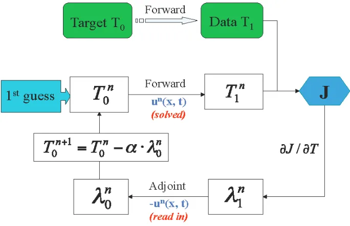
1. Flow chart of the adjoint-forward iterative solver ... 9
2. Adjoint inversion of a 1D linear thermal diffusion process...13
3. Adjoint inversion of a simple 3D problem ...19
4. Convergence of the models shown in Fig. 3... 20
5. Adjoint inversion of a complex 3D problem... 22
6. Convergence of the models shown in Fig. 5 ... 24
7. 3D model with a single viscosity layer ...34
8. Recovery of model parameters for models with a single layer...37
9. Same as Fig. 7 except for a two-layer viscosity... 41
10.Recovery of viscosities given the temperature scaling ...43
11.Same as Fig. 10, except with different temperature scaling ...45
12.Recovery of all model parameters through dynamic topography... 47
13.Farallon remnants revealed by both P and S tomographies ...57
14. Stratigraphic constraints used in the inverse model...59
15. Configuration of the present Farallon remnant slabs ...62
16.An SBI recovery of Farallon subduction ...65
17.A sketch showing the parameterized stress guide...67
18.Recovery of Farallon subduction with the stress guide ...69
19.Convergence of the adjoint iterations...70
20.Subduction inversion with sensitivity tests ...71
21.Constraining the effective temperature through flooding...74
22.Constraining upper mantle viscosity with flooding ...76
23.Constraining upper mantle viscosity with subsidence rates...78
24.More models showing the effects of viscosities on flooding...79
25.Evolution of the Farallon subduction during Late Cretaceous ...83
27.Predicted dynamic topography over North America at 70 Ma...86
28.Present-day Farallon remnant slabs in the lower mantle ...88
29.3D evolution of Farallon slabs in our preferred model...89
30.Maps of pre-Laramide and Laramide features ... 93
31.Proposed models explaining the Laramide Orogeny...93
32.Predicted positions of oceanic plateaus in Late Cretaceous ...96
33.Comparison of Laramide features with plateau subduction ...99
34.Dynamic uplift of the Laramide province...102
35.Surface topography over the subducting Inca plateau ...103
36.Present-day position of the subducted oceanic plateaus ...106
37.Predicted dynamic topography over the western United States ...111
38.Topographic evolution of the southwest Colorado Plateau...113
39. Farallon flat slab beneath North America ...115
40. Migration of Farallon slabs beneath the Colorado Plateau...116
41.Active upwelling and dynamic topography of the CP ...118
42.Geoid low above the subducting Inca Plateau ... 122
43.Observed and modeled subsidence across Utah-Colorado ...125
44.Observed and modeled subsidence across Wyoming ...126
45. New constraints for improving the inverse model...130
46.Comparison between sea-level curves ...133
47.Predictions of the US East coast subsidence...134
48.Reconstructed global subduction from the adjoint model ...138
49.Changes in elevation of S. America along equator since Eocene...140
LIST OF TABLES
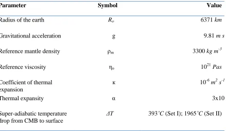
Table 1: Parameters for models in synthetic experiments...15
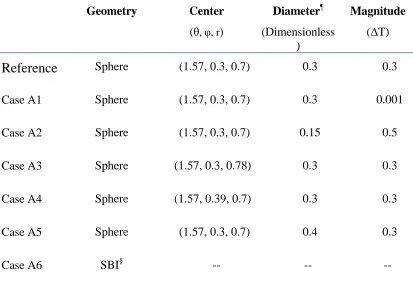
Table 2: Description of the reference initial state and first guesses...16
Table 3: Parameters for models with data assimilation... 62
C h a p t e r 1
Introduction
One of the ultimate goals of geophysics is to understand subsolidus mantle convection and its relationship with surface observables, both geophysical and geological. Steady progress has been made as we increase our ability to image the earth’s internal
structures. Development of seismic tomography has provided significant insights into mantle convection. From global seismic tomography, we see not only large-scale
low-velocity anomalies rising from the CMB and high-low-velocity belts correlated with ancient subduction zones [Su et al., 1994; Li and Romanowicz, 1996; Masters et al., 2000], but also structures like subducted oceanic slabs extending into the lower mantle [Grand et al., 1997;
Van der Hilst et al., 1997; Ritsema et al., 2004; Li et al., 2008]. Deep-rooted columnar low seismic velocity structures, associated with surface hot spots, may have been detected and
could be indicative of active mantle plumes [Montelli et al., 2004, Zhao, 2004; Nolet et al., 2007]. Closer to the surface, regional tomography has imaged active subduction zones showing high seismic velocity slabs overlain by low velocity mantle wedges [Zhao et al.,
1997; Huang and Zhao, 2006; Sigloch et al., 2008; Roth et al., 2008]. Although very informative, tomographic images only provide a snapshot of mantle convection, the final
instant of an evolving system.
In order to constrain the time dependence of mantle convection, other geophysical observations beyond seismic imaging and gravity that extend into the time domain are
1998]. Another possibility comes from surface topography (through stratigraphy and
relative sea level) that has been used as a constraint on time-dependent models of mantle convection [Gurnis, 1993; DiCaprio et al., 2009], some with assimilated plate motions
[Gurnis et al., 1998]. Furthermore, predicting the present-day mantle seismic structures through forward models also helps to constrain past geologic events [Bunge and Grand, 2000] and explain uncertain mantle anomalies [McNamara and Zhong, 2005].
However, previous models of mantle convection have all faced the difficulty of incorporating reasonable initial conditions. For example, Bunge et al. [1998] assumed a
quasi steady-state mantle structure achieved by imposing the Cretaceous plate motion for a relatively long time before allowing time-dependent plate kinematics to start. This assumption is potentially problematic since plate motions change continuously. Gurnis et al.
[1998] used an initial condition at 140 Ma in a model of the Australian region based on the earlier geological evolution. These initial conditions cannot reproduce the exact structures of
present-day mantle.
On the other hand, Steinberger and O’Connell [2000] and Conrad and Gurnis [2003] utilized a simple backward integration of the convection equations to predict past
mantle structure by advecting the current mantle structures back in time, while neglecting thermal diffusion. This method, however, limits its application, because neglecting thermal
diffusion will lead to the accumulation of artifacts at thermal boundaries with time [Ismail-Zadeh et al., 2004]. Inferring the initial condition of a diffusive process through a simple reversal of time is problematic because it leads to exponentially growing numerical errors,
A promising approach to recovering initial conditions is through the use of an
adjoint method widely adopted in meteorology and oceanography [Talagrand and Courtier, 1987] and recently introduced into mantle convection [Bunge et al. 2003; Ismail-Zadeh et
al., 2004]. The method constrains the initial condition by minimizing the mismatch of a prediction to observation iteratively in a least-square sense. Through synthetic experiments, Bunge et al. [2003] and Ismail-Zadeh et al. [2004] separately demonstrated that the initial
condition could be effectively recovered with iterative solver schemes. However, the application to geophysical problems remained limited, because earlier tests all assumed that
the initial condition is the only unknown in the system, which is obviously not true. In fact, both the rheology and effective Rayleigh number of the mantle, two key parameters governing the vigor of convection, are still uncertain, and this prohibits a unique recovery of
the past mantle structure since the solution strongly depends on these mantle properties. On the other hand, the computational expense of earlier adjoint algorithms is high, especially
for large- 3D models.
In this thesis, I will summarize our work on improving the adjoint method by expanding the category of data constraints for assimilation and applying the method with
real data. In Chapter 2, we describe the theoretical basis of the adjoint method in mantle convection and its implementation in computational software. By bringing in
time-dependent observations, i.e., surface dynamic topography, the adjoint method can be used to constrain uncertain mantle dynamic properties, while simultaneously recovering the unknown initial conditions of mantle, as we show in Chapter 3. While in Chapter 4, with the
based on data (including seismic tomography, plate motions, and stratigraphy as proxy for
dynamic topography). The model was tailored for recovering the Farallon plate subduction back to the Late Cretaceous. In Chapter 5, by combining the adjoint models with plate
reconstructions and structural features, we argue that the mechanism causing flattening of the Farallon slab was subduction of two oceanic plateaus, whose passage beneath North America had led the formation of the enigmatic Laramide orogenic event. This chapter also
discusses the vertical motion evolution of the western and eastern U.S. accompanying the Farallon subduction, and implication of the inverse model on quantifying evolution of the
western interior basins. In Chapter 6, I first provide a broader discussion on subduction evolution during the past beyond North America based on the adjoint model we have developed, followed by a summary of limitations of the current inverse models and some
C h a p t e r 2
Adjoint Method in Mantle Convection
12.1 Theoretical Basis of the Adjoint Method
The adjoint method for data assimilation is a gradient-based inversion, which is particularly useful for inverting nonlinear dynamic systems. Derivation of the adjoint
method for an evolving system is based on perturbation theory, where a mismatch in the model output against observation is attributed to an error in the model input, with their
relation approximated as a first order derivative (gradient) of the least-squared mismatch with respect to the input. To formulate the concept mathematically, consider an initial value problem in which all the governing equations and boundary conditions are perfectly
known and numerical errors are negligible. Any mismatch in the prediction should be attributed to errors in the initial condition (i.e., model input). This relation can be simply
expressed as , where J is a scalar cost function, which defines the
mismatch of prediction from data and is the initial variable that potentially carries error. If an explicit form of the expression can be obtained, then the perturbation (i.e.,
error) associated with the initial condition can be retrieved.
Specifically, we define the cost function J as a function of temperature T
where is the predicted temperature, is the actual temperature (with the subscript d denoting data), t is time, and V is volume. In mantle convection, is available only at the present day t1, so effectively J is a delta function in the time domain with a nonzero value at t1.
The governing equations for mantle convection, assuming an incompressible and Newtonian fluid, are
(2)
(3)
(4)
where is velocity, dynamic pressure, dynamic viscosity, ambient mantle
density, coefficient of thermal expansion, temperature anomaly, gravitational
acceleration, temperature, and thermal diffusivity.
If we assume T(t0) is the only variable that brings error into our prediction, our goal, in order to retrieve this quantity, is to obtain the expression J/T(t0), where t0
refers to the initial time. This expression can be obtained through a constraint condition of the energy equation by introducing the adjoint variable (a Lagrangian multiplier) that
forms a Lagrangian function L
A perturbation in L corresponds to perturbations in J and T. Subsequently, we will use
In principle, the velocity u should also contribute to this perturbation since it depends on T (see Eq. 3 and Bunge et al. [2003]), but we choose to neglect the velocity dependence in
Eq. (5’). This is because, first, a full differentiation of Eq. (5) leads to a coupled system of the adjoint and forward models that is numerically changing to implement [Bunge et al.,
2003]; second, inaccuracy from omission of the u dependence in Eq. (5’) is diminished by the variational approach to the single temperature-adjoint solution through iterative schemes we will describe. By applying integration by parts over time and space to Eq. (5’)
with prescribed boundary conditions, we obtain
This is called the adjoint equation or adjoint operator.
In practice, J/T is nonzero only at the final time (t1) in a mantle convection
equation (Eq. 6) is the same as the forward energy equation (Eq. 4) except for the
diffusion term that has an opposite sign. This difference also means Eq. (6) is numerically unstable in describing a forward-time evolution, but ideal for representing a
backward-time process. If we consider t as always being forward in time while substituting Eq. (1), then the differential form of Eq. (6) becomes
the final instant of time (which also provides a state for the system to start with), Eq. (6’) represents a backward-in-time advection-diffusion process.
It can be seen that with Eq. (6), Eq. (5”) can be reduced to
Eq. (7’) indicates that the gradient of the Lagrangian function L with respect to the initial
temperature can be explicitly expressed as the adjoint quantity at the initial time. Since the Lagrantian function is an augmented (constrained) cost function, as can be seen from Eq. (5) where the zero valued constraint (Eq. 4) is prescribed at both t0 and t1, we can conclude that
J
T(t0)=V
(t0)dv (7”)This equation eventually allows for the following numerical algorithm to be reached.
For more references, this adjoint of the energy equation has been derived for meteorological [Sun et al., 1991; Sirkes and Tziperman, 1997] and mantle convection
problems [Bunge et al., 2003; Ismail-Zadeh et al., 2004].
In order to reverse a nonlinear process like mantle convection, iterative solvers are
inevitable. We interleaved the backward adjoint calculation with a forward solution of the energy and momentum equations within an iterative procedure similar to that proposed by Bunge et al. [2003].
Our convention for subscript refers to time (0 for initial; 1 for present) while those for superscripts refer to the number of iterations. The number of iterations is determined by
the accuracy to which we desire our prediction to satisfy data. Specifically these are described in the steps followed:
(i) Solve the forward problem with all three governing equations (Eq. 2 to 4) with
initial condition ( , where n is the iteration number) and predict . The first
initial condition is potentially arbitrary. Store the velocity field for all time steps.
(ii) Compute the mismatch and its gradient ; solve the adjoint energy
(iii) Update the initial field: , where is a damping
factor (defined as in Ismail-Zadeh et al. [2004] except that we took a simple form assuming
only depends on n), with an adjustable integer
(8)
In general, the coefficient can also be a constant with values no more than 0.5, in order to reduce overshoots.
Figure 1 Illustration of the forward- adjoint iterative solver. T0 and T1 represent the reference initial
and final states, respectively. un is velocity for the nth iteration, which is solved during the forward
run and read in from storage during the adjoint run.
the adjoint method, and the present state is the function we try to match with the forward
predictions. The reference states are generated by a forward run that solves the normal convection equations (Eqs. 2, 3, 4). The forward and adjoint iterations follow the procedures
2.2 Numerical Implementation of the Adjoint Method
2.2.1 Solving 1D Linear Problems
Before we apply the adjoint method to more complex problems, we first design a very simple example: to invert a 1D kinematic thermal-diffusion problem, through which
we illustrate the workings of the adjoint method. This simulation is carried out with a code based on the finite-element method (FEM) written in the programming language Matlab.
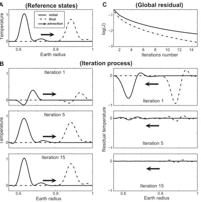
Imagine the reference initial condition is a thermal upwelling, e.g., a mantle plume, situated in the lower mantle sometime in the geological past (Fig. 2A), which is also the target solution we seek by inverting the present-day “observed” structure of this upwelling.
For simplicity, only the forward energy equation (Eq. 4) and its adjoint operator (Eq. 7) are solved, with a prescribed velocity field. Without having to solve the advection term in Eq.
(4), this is essentially a linear problem.
As Fig. 2B illustrates, the first guess of the initial condition has little correlation with the reference, so does the first prediction. This creates the largest mismatch between
prediction and observation (i.e., residual temperature) among all iterations (Fig. 2B and C). The first correction to the initial condition, generated by advecting this large residual back to
the initial time, is also the largest among all iterations. The initial condition, after five updates, becomes much closer to the reference while the mismatch decreases. After 15 iterations, the solution and target converge with a small mismatch. The convergence process is also reflected through a global root-mean-squared (RMS) residual (Fig. 2 C) for the initial
Figure 2 Adjoint inversion of a 1D linear advection-diffusion process. A. Reference initial (solid)
and final (dashed) states, the bold arrow indicates the direction of the prescribed velocity. Both axes
are dimensionless. B. The iterative procedure solving the initial condition. Left column shows the
forward runs, while the right shows the adjoint runs. Three different iterations are shown. C. Global
root-mean-squared residuals from both the initial and final states, as a function of iterations. Note the
Additional tests with different first guesses show that the solution is independent
of prior information about the true initial condition. This indicates the adjoint method convergences to the true solution unconditionally for this linear inverse problem, consistent
with inversion theory [Tarantola, 2005].
2.2.2 Solving 3D Nonlinear Problems
For spherical problems, we have implemented the adjoint algorithm into software
using the finite element and designed specifically for mantle convection, CitcomS [Zhong et al., 2000; Tan, et al., 2006]. The version of CitcomS used here solves the equations within a
spherical geometry and scales well on large parallel computers. Our changes were made to CitcomS version 2.1.0 obtained from the Computational Infrastructure for Geodynamics (https://geodynamics.org).
Upon implementation of the adjoint method within CitcomS, we hope to obtain a good solution to the initial condition while reducing the computational cost as well. Two
sets of numerical experiments are designed that used the forward-adjoint looping to estimate initial conditions. The first set has a uniform viscosity (=1), a constant ambient mantle
temperature, and a Rayleigh number of 1.0108. The second set of experiments has a
layered viscosity, a top thermal boundary layer, and a higher Rayleigh number.
The model domain is: colatitude [1.27, 1.87], longitude [0.0, 0.6] (both in
radians), and radius (normalized by outer radius of the earth) r[0.55, 1]. Boundary
is the outer normal vector, u the velocity vector, and u tg the tangential velocity; the
surface and core-mantle boundary (CMB) are isothermal, while the sidewalls have zero heat flux, n T =0. The adjoint model has zero adjoint temperature on the surface and CMB,
and zero adjoint heat flux on the sidewalls. The Rayleigh number is
Ra=mgRo 3T
o
(9)
where T is the temperature drop from CMB to surface. Time is non-dimensionalized, with
the actual time t related to the model time t’ by
t=t Ro2/ (10)
All symbols with their dimensional values are listed in Table 1. Hereafter, all physical quantities are normalized with their dimensional values, if not noted separately.
2.2.2.1. Models within a single layer
In the first set (Set I) of experiments, the reference states include an initial condition
(Fig. 3A) that has a spherical hot anomaly in the lower part of mantle (with a maximum temperature increase of T = 0.3 at the center and a Gaussian temperature profile across the center). The final condition was produced by running the model forward for 9 Myr (Fig.
3B). These two reference states are the targets we attempted to predict with the adjoint
method. All models are computed on a 333333 grid. We assumed n0 = 1 in Eq. (8), for
Table 1:Summary of Model Parameters
Parameter Symbol Value
Radius of the earth Ro 6371 km
Gravitational acceleration g 9.81 m s
Reference mantle density m 3300 kg m-3
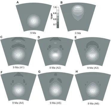
All iterations were started with different first guesses to the target initial condition
(each of these guesses constituted different cases, A1A6, with “A” denoting adjoint
method). Either we assumed a uniform temperature, a temperature that was a function of the
actual initial condition, or generated an estimate through a simple backward integration of the governing equations (hereafter, we refer to this state of the system the SBI). The SBI was obtained by integrating the governing equations from t1 to t0 while reversing the sign of
gravity from the forward calculation. The initial guesses were arranged in order of how close they are to the target initial condition (Table 2). Specifically, Case A1 had a nearly
isothermal condition with a tiny perturbation. Case A2 had an anomaly with the same center as the target, but with a smaller volume (1/8) and hence buoyancy. Cases A3 had the same
Case A4 also had the same shape and buoyancy as the target but its center was shifted
horizontally by 400 km. Case A5 had the same center but the anomaly had a larger volume
(2.4) and hence buoyancy. Case A6 used the SBI first guess to obtain the first guess.
Table 2: Description of the thermal anomaly structures in the reference initial state and various first guesses
Note: SBI§ means simple backward integration, i.e., reverse the sign of gravity and run the forward
model from the present-day mantle structure for the same amount of time.
¶
: Diameter of the spherical anomaly, normalized by Ro, radius of the earth.
For comparison, we ran all cases for 50 iterations while tracking the recovered initial
Case A4 to A6 (Fig. 3FH) were better than those in A1 to A3 (Fig. 3CE). Case A6
gave the best recovery (Fig. 3H). The root-mean-squared (RMS) residuals between the
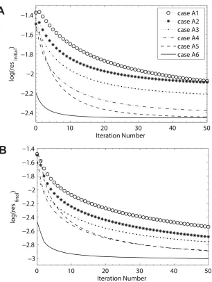
recovered initial conditions and the target initial (Fig. 4A), and those between the predicted and target final (Fig. 4B) decreased with the number of iterations. The terminal (at n = 50) residuals for both the initial and final states (Fig. 4A, B), decreased from Case A1 to A6 as
the first guess more closely reflected the target initial condition. The SBI first guess (A6), especially, started the first iteration with residuals far smaller than the others and the
residuals with the final state remained small in comparison to the other cases (Fig. 4A, B). The rate of convergence was also dependent on the initial guess: the closer the first guess to the target initial condition, the faster the convergence (Fig. 4A, B). The case based on an
SBI first guess was one of the fastest converging cases and required the least number of iterations to converge. If the final solution is achieved when the slope of the residual
between predicted and target final decreases to below a specified small value, then solving for the initial condition with the SBI first guess is almost an order of magnitude faster than the others. The convergence of Case A1, with the nearly isothermal initial condition, is far
smaller than A6 using the SBI first guess and much of this difference arises from the organization of the forward-adjoint looping. For Case A1, the adjoint temperature at t1 is
nearly the negative of the final temperature, in other words, almost possessing the same buoyancy used in the strict reverse calculation (SBI first guess). However, when the adjoint temperature in A1 is advected from t1 to t0, the stored velocity field from the forward
guess overcomes this limitation by using the velocity field from the actual backward
calculation.
Figure 3 Three-dimensional forward-adjoint models (with a 333333 mesh) for a mantle with a
single-layer viscosity and uniform background temperature. Shown is temperature for vertical
cross-sections along lines of latitude through center of the domain.Reference thermal states at 9 Ma (A)
and present (B). (C to H) Retrieved initial states at 9 Ma using six different initial guesses (Case
Figure 4 Convergence of the models shown in Fig. 3. (A) Root-mean-squared (RMS) residuals of
recovered initial conditions with respect to the reference initial versus iteration. (B) RMS residuals of
the predicted final conditions with respect to the reference final versus iteration.
Since the solutions are dependent on the first guess, finding the optimal one is
important to decrease the computational cost while obtaining a reasonable solution. Because the SBI first guess gives the best solution to the initial condition, both in terms of the
obtain an optimal first guess. Another advantage of obtaining the first guess via the SBI is
that it requires no a priori information of the solution. Algorithmically, it is also easy to obtain.
2.2.2.2. Models with thermal boundary layers and depth- and
temperature-dependent viscosities
The second set (Set II) of experiments is geophysically more realistic with a top
thermal boundary layer (TBL) representing the lithosphere and a four-layer mantle with temperature-dependent viscosity. The TBL has an error function temperature profile typical
of 40 Ma oceanic lithosphere. The viscosities for lithosphere, asthenosphere, transition zone, and the lower mantle, without temperature-dependence, are 10, 1, 10, and 40, respectively. The temperature dependence of viscosity is
T =oexp( 1
T+0.31) (11)
where Tis temperature-dependent viscosity and o is the depth-dependent prefactor. This
results in an order of magnitude decrease in viscosity from T=0 to 1. Compared to Set I, we
used a higher Rayleigh number at 5.0108.
The target initial condition has the same thermal anomaly as that in model Set I, only that it has a TBL on top (Fig. 5A). The target final condition (Fig. 5B) is 52 Myr after the
TBL as in the target initial. Case A6 is with the SBI first guess. Comparatively, these first
guesses in AL1AL5 had more information on the target initial than those in A1A5,
because we assumed the correct TBL in these guess. On the other hand, Case AL6 (using the SBI first guess) had less information on the initial condition because the TBL had to be entirely recovered with the forward-adjoint looping. All models were realized with a
494949 mesh with an under resolved lithosphere spanned with just two mesh points.
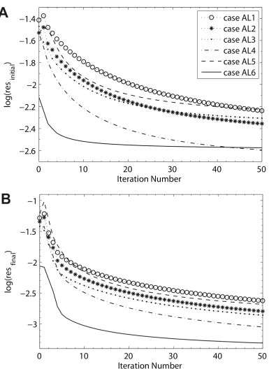
Figure 5 Three-dimension forward-adjoint models (with a 494949 mesh) for a model with a
radially stratified viscosity and a top thermal boundary layer. Shown is temperature through vertical
cross-sections. Reference states at 51.5 Ma (A) and present (C). (B) Radial viscosity profiles in the
reference initial condition. (D to I) Retrieved initial states from six different initial guesses (AL1–
AL6) after 50 iterations.
Since these models are more complex, and thus more nonlinear, than models in Set I, a smaller damping factors with no = 2 is adopted, in order to avoid overcorrection in the iterative process. We integrated the forward and adjoint equations for 50 iterations to obtain
the solutions (Fig. 5CH). Since the temperature field includes a TBL and a lower mantle
anomaly, a small residual would entail recovering both well. The comparison of recoveries in these cases is not as obvious as that of only a rising Stokes sphere (Set I). Case AL5 with the closest initial guess also accumulated substantial errors through the nonlinear interaction
between the rising spherical anomaly and the thermal erosion of the lithosphere. Case AL4 and AL6 both gave good recoveries with the smallest residuals between recovered and target
initial condition (Fig. 6A), and AL6 among all cases had smallest residual between predict and target final condition (Fig. 6B). The SBI first guess (AL6) also led to fastest convergence, and most of the residuals were reduced within the first 10 iterations. From
Other experiments showed that by increasing no, hence decreasing , we could
decrease the terminal residuals of the initial condition in AL1 to AL5 upon convergence, some of which (AL4 and AL5) could be even smaller than in AL6, indicating a better
recovery, but the terminal residual of the final condition in AL6 was always the smallest. However, for these tests, we had to increase the number of iterations to obtain the same amount of reduction of residuals; in other words, we reduced the rate of convergence
substantially in A1 to A5, while A6 always had the fastest convergence and smallest residuals during most of the iterations. This indicates that the SBI first guess always
produces good solutions with the least computational cost
2.2.3 Discussion
Inferring initial conditions with adjoint methods for mantle convection seems inherently ambiguous compared to atmospheric circulation problems where direct constraints on initial conditions from measurements in the system interior are used. Using a
technique similar to that in Bunge et al. [2003], we first inferred initial conditions via the looping between forward and adjoint calculations to minimize the difference between a
prediction and the final state of the mantle (a state that can be determined from seismic tomography). An optimal convergence requires some constraint on the initial condition. Starting the first forward calculation with an isothermal mantle was less efficient than with
and distorts a thermal boundary layer, where diffusion is important, the SBI first guess
continues to provide a good estimate for the initial condition.
The adjoint method is an iterative gradient method that solves for a linearized
problem. For the final solution to reach the global minimum in the residual space, the trial solution in the first iteration must be close to the true solution. Since the SBI initial guess makes use of present-day mantle information, this inverse of mantle convection
approximates the true solution to first order. Therefore, the SBI initial guess guarantees a good solution with the adjoint method, as long as the model has not been run so long that
diffusion at boundary layers dominates the problem. However, the approximation of initial conditions based on SBI will face difficulty when the anomalies reach a thermal boundary layer (TBL) and gradually diffuse away, which means an SBI estimate will not provide the
same amount of buoyancy force. This is the natural limit for the adjoint method [Ismail-Zadeh et al., 2004].
The SBI initial guess is close to optimal for most mantle convection problems because advection dominates thermal diffusion with typical Peclet numbers ~103. To best approximate the true solution, an initial guess must capture its total buoyancy and geometry
that we demonstrated with several numerical experiments in which either the buoyancy was underestimated or the initial location was incorrect. In these cases, the trial solutions all have
large initial errors that must be iteratively removed with forward-adjoint looping. An idealized case with the correct initial location and buoyancy that is close to the actual initial condition recovers the initial condition nearly as well as with the SBI first guess. Since the
obtain a condition that has almost the same total buoyancy as that in the true solution and
with its geometry defined through the coupled solution of flow and advection; this initial guess will, of course, lead to a good solution.
Seismology has revealed that the mantle has both low and high velocity regions that putatively represent a complex combination of thermal and chemical anomalies [Masters et al., 2000; Ishii and Tromp, 1999; Ni et al., 2002]. In these real cases where mantle
anomalies have irregular geometry and amplitude, arbitrary initial guesses can hardly capture the true solution in the first place, and the SBI initial guess will be especially
beneficial in retrieving a reasonable representation of the true initial condition.
However, it is worthwhile to point out that the tests performed in this chapter all assume that mantle properties, including the viscosity distribution, constitutive relation, and
mantle density anomalies are perfectly known. In other words, these are idealized situations, which do not exist in the earth. For geophysical problems, many other unknowns need to be
solved. Besides the dynamic properties like mantle viscosity and density anomaly, chemical composition and its temporal variation are other questions requiring solution. The numerical experiments shown in this chapter all treat mantle density anomalies as being thermal in
C h a p t e r 3
Constraining Dynamic Properties of Mantle
23.1 Need for Assimilation of Time-Dependent Data in Real Problems
Unlike atmospheric or oceanographic problems where many parameters within the
interior of the flow can be measured and calibrated in situ, dynamic parameters for the mantle convection problem are obtained indirectly. A good example of such a parameter is
the depth dependence of mantle viscosity, unfortunately a parameter that remains uncertain [Walcott, 1973; Hager and Clayton, 1989; Steinberger and O’Connell, 2000; Mitrovica and Forte, 2004]. This of course is problematic for the adjoint problem described in
Chapter 1, because what viscosity should be used for the recovery of initial conditions? Another critical parameter for recovery is the magnitude of the temperature (density)
within the anomalies. Clearly, important constraints can be placed on this problem from seismic tomography, but high-pressure, high-temperature laboratory experiments have not achieved the ability to uniquely map seismic into thermal anomalies. Thus, even for simple
convection models, we should consider these basic model parameters to have uncertainty when the adjoint method is used to infer initial conditions.
As discussed in Chapter 1, a quantitative description of the time dependence of mantle flow requires time-dependent constraints. Here I will explore the surface dynamic
topography, a different type of observation from plate motions used in earlier studies
[Lithgow-Bertelloni and Richards, 1998]. With the adjoint method implemented in CitcomS, we can compute the prior history of thermal anomalies for a given viscosity
model and present-day mantle thermal structure. From the restored history, we then predict dynamic topography that can be constrained through stratigraphic constraints, such as tectonic subsidence from boreholes [Heller et al., 1982; Pang and Nummedal, 1995],
paleo shorelines [Bond, 1979; Sandiford, 2007; DiCaprio et al., 2009], and sediment isopachs [Cross and Pilger, 1978]. Given these additional observational constraints, there
is the opportunity to place limits on mantle viscosity and temperatures.
3.2 Dynamic Topography Constrains Uncertain Mantle Properties
For this study, we designed two sets of synthetic experiments, one for a simple one-layer mantle with uniform viscosity, and the other for a two-layer mantle viscosity structure.
3.2.1 One-Layer Mantle
First let us consider a mantle with a uniform viscosity throughout. On the top
surface of the convection model, dynamic topography, h, is defined from
(12)
where is the total normal stress in the radial direction and is the density contrast
across the top surface (implicitly assuming that air overlies the solid mantle). At any instant
of time, normal stress is proportional to the temperature scaling (see Eq. 3). For an
inverse problem where we use the present-day seismic tomography to interpret mantle temperature structure, is the temperature magnitude obtained by mapping seismic
velocity variations to thermal anomalies. Together with Eq. (12), we relate dynamic topography with a temperature scaling via a time-dependent coefficient with units, m/K.
The quantity describes the response of surface dynamic topography with a scaled temperature distribution and mantle rheology structure.
(13)
The rate of change of dynamic topography , however, is related to the absolute viscosity
is proportional to the product of and mantle flow speed (i.e., ). In
a Stokes fluid, is proportional to and inversely proportional to mantle viscosity .
Considering Eq. (13), we obtain
(14)
For an inverse problem where and are unknowns, and h(t) and are data
constraints, we simplify the problem by rewriting Eq. (14) with Eq. (13)
(15)
where h1=h(t1), with t1 representing present-day time; (or ’) is a kernel that describes the response of the rate of change of surface dynamic topography assuming a specific mantle viscosity; has units of Pa/m. Instantaneously, when the temperature and viscosity
structures remained unchanged, Eq. (15) was validated numerically for systems with temperature- and depth-dependent viscosities [Gurnis et al., 2000].
Because h(t) and are potentially two independent constraints, and Eq. (13) and
(15) each has an independent unknown, and , respectively, the independent unknowns
might be recoverable. By using h1 instead of h(t) on the right-hand side of Eq. (14), we attempt to partially decouple this two-variable, two-constraint system. Essentially, we use
the magnitude of topography h(t) to constrain (Eq. 13), and use its rate of change to
constrain (Eq. 15).
The left-hand sides of equations (13) and (15) are time dependent. On the
which are evaluated numerically. At any moment of time, and can be found from the
solution of Eq. (2) (4) and are dependent on the viscosity and temperature distribution.
Evaluation of requires two successive solutions of Eq. (2) (4)so that can be found.
Assuming the “structure” of the present-day temperature field is the same as the structure obtained from seismic tomography, we now show how Eq. (13) and Eq. (15) can
be incorporated within an iterative scheme to solve for the unknowns and based on
observed and predicted h(t) and . Define j to be the index of a loop used to refine
temperature and viscosity, while i remains the index over time as it was in the forward-adjoint looping (Sec. 3). At any given time i in loop j, the numerical values of the two
kernels and are computed as , , respectively. Here we
treat two kernels as implicit Green’s functions. and are updated by a method that is
similar to back-projection used in seismic topography [Rowlinson and Sambridge, 2003], the difference being the use of implicit coefficients ( and ) in this case.
(16)
(17)
where m and n are the numbers of sample points within the time series and are potentially different because of the different number of constraints on topography and its rate of
change; subscript d refers to data (observational constraints); and are two damping
This iteration is at a higher level than that of forward-adjoint looping and we
refer to it as the outer iteration. Essentially, seismic tomography at the present day is used to constrain the geometry or depth distribution but not the precise amplitude of mantle
temperature anomalies, and the forward-adjoint looping is used to find that geometry during earlier times. The outer looping is used to refine both the scaling between seismic velocity variations and temperatures (or density) and the viscosity distribution. The whole procedure
is divided into two parts:
(i) Inner loop: While and (without varying temperature dependence) remain
constant, perform an adjoint calculation to recover the initial condition with the SBI first
guess, and predict the dynamic topography during the final iteration.
(ii) Outer loop: Update and via (16) and (17) through the mismatch of the
predicted and target dynamic topography and its rate of change.
The whole procedure is terminated upon convergence of the two model parameters.
In a synthetic experiment, a cold spherical anomaly sinks from top to bottom of the mantle within a 3D spherical region; the system has initial (Fig. 7A) and final reference
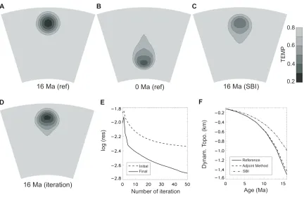
Figure 7 3D models with a single viscosity layer (modeled with a 333333 mesh). Reference
thermal states at 16 Ma (A) and the present (B). (C) First guessed initial condition with a simple
backward integration (SBI). (D) Recovered initial condition with the adjoint method after 50
iterations. (E) RMS residuals for the initial and final states based on the adjoint method. (F) The
predicted dynamic topography histories based on an SBI first guess and the adjoint method,
compared against the reference dynamic topography. All calculations assume a known viscosity
structure.
To illustrate the effect of forward-adjoint iteration on dynamic topography, we ran
the inner loop described above assuming that the temperature scaling and the absolute value of viscosity are known. The SBI initial guess (Fig. 7C) is more diffused in comparison to the finally recovered initial condition after 50 iterations (Fig. 7D). The adjoint method reduces
(Fig. 7E). Consequently, the associated dynamic topography curves from t0 to t1 are also
notably different (Fig. 7F). The curve from the SBI case deviates from the reference much more than the one from the recovered solution, with a maximum deviation in magnitude by
35% vs. 5% of the reference value at 16 Ma. Although the SBI is a good method to find the best first guess for the forward-adjoint looping, the experiment demonstrates that the simple backward advection of the anomaly (SBI) does not perfectly predict the evolution of
dynamic topography.
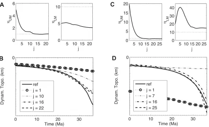
We then started the outer loop with two initial models (Cases AH1 and AH2) in
which the temperature scaling and mantle viscosity had “guessed values” that were
different from the reference ones. The initially guessed parameters of Case AH1 (Fig. 8A, B at loop 1) were such that its effective Rayleigh number was equal to the actual Ra for the reference state while Case AH2 (Fig. 8E, F at loop 1) had an effective Rayleigh number four
times smaller. In both cases, we applied the two-level looping algorithm. The inner loop was applied so that the iteration always started with the SBI first guess, and the number of
forward-adjoint iterations increased as the index of the outer loop increased. We applied this simplification because the first recovered initial condition was not well known before the
constraints on h(t) and were applied. Due to the initially under-estimated temperature
scaling in both AH1 and AH2, the first predicted temporal dynamic topography curves
had small magnitudes and slopes. By applying the outer loop upon the predicted and
reference dynamic topography (Fig. 8C, G), we updated model parameters and . The
difference in magnitudes of topography h(t) forced to increase in both cases where AH2
day magnitude of topography h1 updated the viscosity. The apparently smaller slope in
AH1 was actually larger than that of the reference when normalized by h1, and hence forced the viscosity to increase. The initial smaller slope for dynamic topography in AH2 forced
the viscosity to decrease, and the smaller magnitude forced temperature to increase, overshooting the reference temperature. The overshot was corrected as the viscosity also approached the true value. As a result, for both Case AH1 and AH2, the temporal (Fig. 8C,
G) and spatial (Fig. 8D, H) distribution of dynamic topography converged to the target curves as the two incorrectly guessed model parameters converged to the reference values
after a finite number of loops (Fig. 8A, B and E, F). Most of the model corrections occurred within the first 10 outer loops.
As discussed in Chapter 1, due to the artificially defined initial condition and low
resolution of meshing, the recovered initial condition by the adjoint method is not exact, even with the same model that generates the reference states (Fig. 7D). This effect shows up
in the recovered model parameters as a deviation of viscosity from the reference value by about 2% and that of the temperature scaling by about 1%. However, the final solutions in
both Case AH1 and AH2 are almost identical, indicating the two-level algorithm can both recover initial conditions and unknown material properties.
Under highly controlled set of circumstances, this test shows that the history of the dynamic topography is a valuableconstraint on mantle viscosity and magnitude of present day mantle thermal structures. We will then explore the limitations of this conclusion under
Figure 8 Recovery of model parameters using dynamic topography for models with a single layer.
The starting model has either the same effective Rayleigh number (AD, Case AH1) or a Rayleigh
number four times smaller (EH, Case AH2) than the reference value. All results plotted with
respect to the outer loop index (k) and are computed from the last iteration of the inner
(forward-adjoint) looping. Shown from top to bottom are the temperature scaling (A, E), viscosity (B, F),
temporal evolution of dynamic topography recorded at one point on the surface (C, G), and
3.2.2 Two-Layer Mantle
We now consider the geophysically more relevant possibility of a layered mantle
viscosity [Hager, 1984; Mitrovica and Forte, 1997]. We used a two-layer mantle and
attempted to recover three variables: (present-day temperature anomaly), (upper
mantle viscosity), and (lower mantle viscosity). Given this potentially underdetermined
problem, we determine what we might hope to recover.
For a thermal anomaly within the upper mantle, the upper mantle viscosity controls the flow velocity, , and the evolving dynamic topography. Assuming that the density
anomaly has not yet entered the lower mantle the system has only two variables, and
, just like the isoviscous mantle discussed above. This assumption is not entirely true
since the h does depend on the ratio of upper to lower mantle viscosity [Richards and Hager, 1984; Hager, 1984]. Approximately, we still have the linear relation between h(t) and ,
Eq. (13), and the following relation for , which is similar to Eq. (14)
(18)
For a density anomaly within the lower mantle, the flow speed is approximately inversely
proportional to , and the surface normal stress that defines h(t) is proportional to . So
Eq. (13) becomes
(19)
where , is the ratio of upper to lower mantle viscosity. Consider a static
( ), while Eq. (13) is linear since is not a function of . This implies the inverse
problem for a two-layer viscosity mantle is more nonlinear than for a single layer mantle.
The relation , together with Eq. (19), leads to the expression
(20)
where h1 is dynamic topography at the present day. Again, we use h1 instead of h(t) on the
right-hand side of Eq. (20) to avoid the sharing of data constraints. In fact, Eq. (18) and (20) are equivalent: replace with h1 in Eq. (18) and Eq. (20) is obtained. This shows that the
rate of change of dynamic topography should be a good constraint on the upper mantle viscosity.
Rearranging and discretizing Eq. (20) lead to
(21)
For the other two variables, and , we have constraint equations (13) and (19).
Ideally, we could use Eq. (13) to constrain by assimilating topographic data associated
with density anomalies crossing the upper mantle through Eq. (16). Equation (19) could be
used to constrain by topographic data with lower mantle anomalies iteratively
(22)
In Eq. (21) and (22), m and l are the numbers of sample points within the time series; and
; vi and wi are weighting functions that change with time. We assumed
that vi (wi ) decreases(increases) linearly from i = 1 to l.
However, because a thermal anomaly will move faster in the upper mantle than in the lower mantle, a topographic history would be more heavily weighted in time for the
lower mantle, where largely trades off with when using the dynamic topography
(see Eq. 19). In other words, temperature anomaly and lower mantle viscosity are coupled for most of the topographic record.
Therefore, in order to simultaneously invert for all three variables, we should avoid the trade-off between temperature scaling and lower mantle viscosity. We designed a three-level iterative scheme which solves for all three parameters while minimizing potential
trade-offs between them:
(i) Inner level: While , and remain fixed, perform forward-adjoint looping to recover the initial condition.
(ii) Middle level: While remains fixed, update and via Eq. (21) and (22) through the mismatch of the predicted and target dynamic topography and its rate of change.
(iii) Outer level: Update according to Eq. (16).
The whole procedure is terminated upon convergence of the three model parameters.
For an explicit example, we consider a 2D model that simulates a subduction scenario, where a fragment of a cold slab sinks from the upper mantle into the low mantle
1998] and using the mismatch between observed and predicted quantities will be more
involved than what the experiment given below suggests.
Figure 9 Same as Fig. 7 except for 2D models (on a 129129 mesh) with a two-layer viscosity. The
dashed lines (AD) indicate the upper and lower mantle interface.
To avoid numerical artifacts, we generated the initial condition by first defining a smooth slab on the surface and then allowing the slab to sink to the position shown in Fig.
7a. A fine resolution mesh with a 129129 grid is used, to mimic the trench-normal
identical to the reference initial state. Moreover, the dynamic topography associated with
the SBI estimate deviates from the reference by about 20% at 36 Ma while that with the recovered solution is less than 1%. This indicates that the recovered initial condition with
simple forward-adjoint looping is almost perfect if the viscosity and temperature scaling are known a priori.
Since the inner level involving the forward-adjoint looping has been described in
Section 2.2.1, we focus our discussion on the middle and outer levels. For the middle level, we show several cases with different values, where upper and lower mantle viscosities
are recovered from several initial guesses.
In a set of experiments, we chose at its reference value but incorrectly guessed both viscosities. We tried two starting viscosity models, AH3 and AH4, that were both
guessed to be isoviscous with ( , ) = (5, 5) and (20, 20), respectively, while the target
had a layered viscosity, ( , ) = (1, 10) (Fig. 10A, C). Because the initial upper/lower
mantle viscosity ratio was overestimated in both models, Eq. (19) implies that the
present-day dynamic topography should be overpredicted, as verified as loop 1 in Fig. 10B, D. Since
was controlled by the magnitude of topography during the later part of its evolution, the
over predicted magnitude of h caused to increase (Fig. 10A, C). Since the upper mantle
viscosity was over-estimated in both AH3 and AH4, the rate of the change of
topography was small during the early stages of evolution (Fig. 10B, D). This difference
forced to decrease quickly in both cases. Changes in both and likewise reduced
AH4, first overshot the target (Fig. 10C). This overshoot happened because was
forced to increase at the beginning due to an initially overpredicted h, but as decreased
the viscosity ratio went below the reference, h became underpredicted, which led to the final
decrease of . As the viscosities converged, the topographic evolution conformed to the
target in both cases after a finite number of loops (Fig. 10B, D). We conclude that the
solution is potentially robust as it does not depend on the initial models. Additional experiments demonstrate that solution errors of both upper and lower mantle viscosities are within 1%.
Figure 10 A two-level looping for recovery of both viscosities and initial condition, with
temperature scaling at its reference value. Evolution of upper and lower mantle viscosities with
reference values. (B, D) Convergence of temporal dynamic topography recorded at one point for
Case AH3 and AH4, respectively.
With another set of experiments with all target values as those just described (AH3 and AH4), we incorrectly guessed so that it was either smaller (AH5) or larger (AH6)
than the true value by 50%. AH5 started with an initially isoviscous state, ( , ) = (5,
5) (see Fig. 11A, loop 1); and AH6 started with a higher viscosity, ( , ) = (20, 20)
(see Fig. 11C, loop 1). The initial models were chosen such that their effective Rayleigh
numbers were not too far from the target values. Parameter recovery in these two cases was
similar to what we observed above. Although the viscosity ratio was the same in both
AH5 and AH6, the present-day dynamic topographies were different in loop 1, in proportion
to the different temperature scaling (Eq. 19). Consequently, lower mantle viscosities
evolved very differently when the temperature was incorrectly guessed. In both Case
AH5 and AH6, converged solutions for both viscosities and dynamic topography were obtained. However, although the recovered upper mantle viscosities were always close, there was a tradeoff between lower mantle viscosity and the temperature scaling, as
expected from Eq. (19). With more tests on different initial viscosity models, we found that the solutions were robust in that the converged viscosities oscillated around some mean
values by no more than 5%. Deviations of the topographic evolutions from the target are
instructive (Fig. 11B, D): Due to the tradeoff between and , the later portion of the
predicted curve (closer to present day) always matched the reference curve; however the
Specifically, the earliest portion of the curve was flatter than the reference when was
smaller, and steeper when larger.
Figure 11 Same as Figure 10, except that the temperature scaling is either smaller (A, B, Case AH5)
or larger (C, D, Case AH6) than the reference value by 50%.
This deviation in topographies during the early part of evolution is the basis of an outer level iteration for the update of . When is incorrect, lower mantle viscosity
trades off with temperature, upper mantle viscosity does not; in theory, dynamic topography can never be predicted exactly if is incorrect. Eq. (13) and (18) imply that different , lead to different early topographic evolutions. In practice, we used the very simple relation
described by Eq. (13) to update , constrained from the deviation described above. The iterative relation is given by Eq. (16), where n is the number of data points within the time
topography, we used the amount of change of topography from the initial time to the nth
point. Essentially, we use the difference in the slope at the initial stage of subduction.
As an example, we used the values of in AH5 and AH6 as two starting guesses
for the temperature scaling, and then applied an additional outer loop (calling these new cases, AHT1 and AHT2). The procedure for the outer loop is described above. Note that with different values of , the converged dynamic topography had different slopes at
initial times. We calculated the mismatch between the predicted and reference dynamic topography over the early part of topographic evolution and applied Eq. (16) to update .
Consequently, the deviated topographic curves in both AHT1 (Fig. 12A) and AHT2 (Fig. 12E) moved toward the reference as the number of outer loops increased. Convergence of ’s were shown in Fig. 12B and F with respect to outer loop, where the symbol size was
proportional to the residual between predicted and reference dynamic topography. Both the evolution of topography and that of indicated a correct convergence. To show the
interior process of this three-level looping scheme, we picked some value of during the evolution as an example. For this , we plotted the updating mantle viscosities, i.e., the middle level loop (Fig. 12C, G). When the two viscosities converged, the corresponding
RMS residuals between predicted and target mantle thermal structure at the initial and final (present-day) time also converged (the innermost loop, Fig. 12D, H). These experiments
illustrate well that when is incorrect, recovered is also incorrect; recovered mantle
scaling in both cases approximated its target value within 1%. How closely the final
solution fits the reference values will be affected by the discretization of data and the form of weighting functions in Eq. (16), (20), and (21). In the final solution, all recovered model
parameters have errors less than 1%, where the lower mantle viscosity linearly trades off with temperature scaling.
Figure 12 The three-level looping algorithm shown for Case AHT1 (AD) and AHT2 (EH), with i,
j and k denoting the index of inner, middle, and outer loops, respectively. Shown are evolution of
topography at the earliest time (A, E) and temperature scaling (B, F) with respect to outer loop,
convergence of upper and lower mantle viscosities versus middle loop, and RMS residuals for both
F, the size (area) of the open circles correspond to the mismatch between magnitudes of predicted
and reference dynamic topography in A and E, respectively. All dashed lines indicate the target
values.
In summary, our experiments show that, given a temporal record of surface dynamic
topography and the present-day mantle seismic tomography showing the geometry of anomalies, this three-level looping scheme allows the recovery of all three mantle dynamic parameters, including upper mantle viscosity, lower mantle viscosity, and the magnitude of
the temperature anomaly scaled from seismic perturbations.
3.2.3 Discussion
Combined with dynamic topography observations, the application of the adjoint method can be expanded so that not only can past mantle structures be recovered but also
constraints placed on mantle properties. Based on the governing equations, we developed multi-level iteration schemes that constrain both mantle thermal anomalies (the scaling
between seismic velocity and temperature or density) and absolute values of upper and lower mantle viscosities. With synthetic experiments, we show that our algorithm is stable and robust. It is worthwhile to note that although this algorithm allows all three model
parameters to vary while the final solution remains unique (the uniqueness depends on the recovering power of the adjoint method). In practice, however, we should take advantage of