Thesis by
Hsuan-Tien Lin
In Partial Fulfillment of the Requirements for the Degree of
Doctor of Philosophy
California Institute of Technology Pasadena, California
2008
Acknowledgements
First of all, I thank my advisor, Professor Yaser Abu-Mostafa, for his encouragement and guidance on my study, research, career, and life. It is truly a pleasure to be embraced by his wisdom and friendliness, and a privilege to work in the free and easy atmosphere that he creates for the learning systems group.
I also thank my thesis committee, Professors Yaser Abu-Mostafa, Jehoshua Bruck, Pietro Perona, and Christopher Umans, for reviewing the thesis and for stimulating many interesting research ideas during my presentations.
I have enjoyed numerous discussions with Dr. Ling Li and Dr. Amrit Pratap, my fellow members of the group. I thank them for their valuable input and feedback. I am particularly indebted to Dr. Ling Li, who not only collaborated in many projects with me throughout the years, but also gave me lots of valuable suggestions in research and in life. Furthermore, I want to thank Lucinda Acosta, who just makes everything in the group much simpler.
Special gratitude goes to Professor Chih-Jen Lin, who not only brought me into the fascinating area of machine learning eight years ago, but also continued to provide me very helpful suggestions in research and in career.
I thank Kai-Min Chung, Dr. John Langford, and the anonymous reviewers for their valuable comments on the earlier publications that led to this thesis. I am also grateful for the financial support from the Caltech Center for Neuromorphic Systems Engineering under the US NSF Cooperative Agreement EEC-9402726, the Caltech Bechtel Fellowship, and the Caltech Division of Engineering and Applied Science Fellowship.
Abstract
We study the ordinal ranking problem in machine learning. The problem can be viewed as a classification problem with additional ordinal information or as a re-gression problem without actual numerical information. From the classification per-spective, we formalize the concept of ordinal information by a cost-sensitive setup, and propose some novel cost-sensitive classification algorithms. The algorithms are derived from a systematic cost-transformation technique, which carries a strong the-oretical guarantee. Experimental results show that the novel algorithms perform well both in a general cost-sensitive setup and in the specific ordinal ranking setup.
From the regression perspective, we propose the threshold ensemble model for ordinal ranking, which allows the machines to estimate a real-valued score (like re-gression) before quantizing it to an ordinal rank. We study the generalization ability of threshold ensembles and derive novel large-margin bounds on its expected test performance. In addition, we improve an existing algorithm and propose a novel al-gorithm for constructing large-margin threshold ensembles. Our proposed alal-gorithms are efficient in training and achieve decent out-of-sample performance when compared with the state-of-the-art algorithm on benchmark data sets.
reduction framework results in a novel and faster algorithm for ordinal ranking with superior performance on real-world data sets, as well as a new bound on the expected test performance for generalized linear ordinal rankers. Coupling AdaBoost with the reduction framework leads to a novel algorithm that boosts the training accuracy of any cost-sensitive ordinal ranking algorithms theoretically, and in turn improves their test performance empirically.
Contents
Acknowledgements iii
Abstract v
List of Figures ix
List of Tables x
List of Selected Algorithms xii
1 Introduction 1
1.1 Supervised Learning . . . 1
1.2 Ordinal Ranking . . . 7
1.3 Overview . . . 10
2 Ordinal Ranking by Cost-Sensitive Classification 12 2.1 Cost-Sensitive Classification . . . 12
2.2 Cost-Transformation Technique . . . 14
2.3 Algorithms . . . 22
2.3.1 Cost-Sensitive One-Versus-All . . . 23
2.3.2 Cost-Sensitive One-Versus-One . . . 26
2.4 Experiments . . . 31
2.4.1 Comparison on Classification Data Sets . . . 31
3 Ordinal Ranking by Threshold Regression 36
3.1 Large-Margin Bounds of Threshold Ensembles . . . 38
3.2 Boosting Algorithms for Threshold Ensembles . . . 46
3.2.1 RankBoost for Ordinal Ranking . . . 47
3.2.2 ORBoost with Left-Right Margins . . . 50
3.2.3 ORBoost with All Margins . . . 53
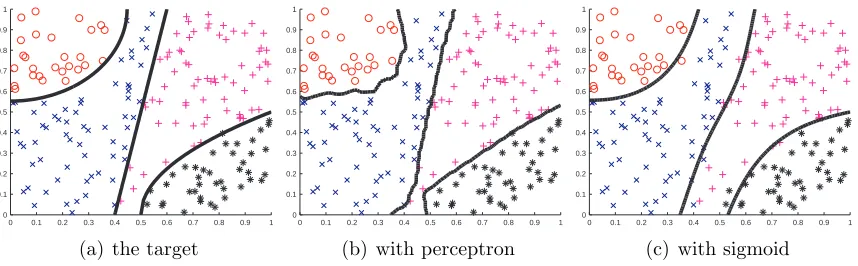
3.3 Experiments . . . 54
3.3.1 Artificial Data Set . . . 55
3.3.2 Benchmark Data Sets . . . 55
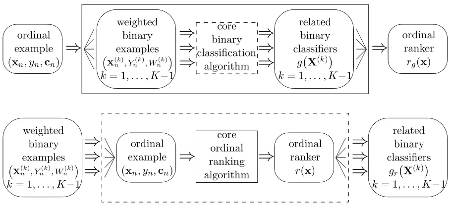
4 Ordinal Ranking by Extended Binary Classification 58 4.1 Reduction Framework . . . 59
4.2 Usefulness of Reduction Framework . . . 69
4.2.1 SVM for Ordinal Ranking . . . 70
4.2.2 AdaBoost for Ordinal Ranking . . . 74
4.3 Experiments . . . 79
4.3.1 SVM for Ordinal Ranking . . . 80
4.3.2 AdaBoost for Ordinal Ranking . . . 82
5 Studies on Binary Classification 87 5.1 SVM for Infinite Ensemble Learning . . . 87
5.1.1 SVM and Ensemble Learning . . . 88
5.1.2 Infinite Ensemble Learning . . . 91
5.1.3 Experiments . . . 96
5.2 AdaBoost with Seeding . . . 101
5.2.1 Algorithm . . . 102
5.2.2 Experiments . . . 103
6 Conclusion 106
List of Figures
1.1 Illustration of the learning scenario . . . 3 3.1 Prediction procedure of a threshold ranker . . . 37 3.2 Margins of a correctly predicted example . . . 39 3.3 Decision boundaries produced by ORBoost-All on an artificial data set 55 4.1 Reduction (top) and reverse reduction (bottom) . . . 64 4.2 Training time (including automatic parameter selection) of SVM-based
List of Tables
2.1 Classification data sets . . . 31
2.2 Test RP cost of CSOVO and WAP . . . 33
2.3 Test absolute cost of CSOVO and WAP . . . 33
2.4 Test RP cost of cost-sensitive classification algorithms . . . 34
2.5 Test absolute cost of cost-sensitive classification algorithms . . . 34
2.6 Ordinal ranking data sets . . . 35
2.7 Test absolute cost of cost-sensitive classification algorithms on ordinal ranking data sets . . . 35
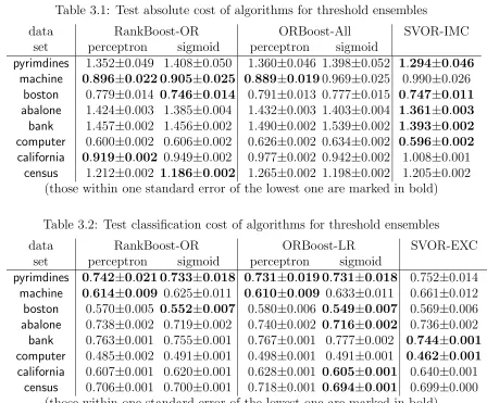
3.1 Test absolute cost of algorithms for threshold ensembles . . . 56
3.2 Test classification cost of algorithms for threshold ensembles . . . 56
4.1 Instances of the reduction framework . . . 70
4.2 Test absolute cost of SVM-based ordinal ranking algorithms . . . 80
4.3 Test classification cost of SVM-based ordinal ranking algorithms . . . . 80
4.4 Test absolute cost of SVM-based ordinal ranking algorithms with the perceptron kernel . . . 82
4.5 Test absolute cost of all SVM-based algorithms . . . 83
4.6 Test classification cost of all SVM-based algorithms . . . 83
4.7 Training absolute cost of base and AdaBoost.OR algorithms . . . 86
4.8 Test absolute cost of base and AdaBoost.OR algorithms . . . 86
5.1 Binary classification data sets . . . 98
5.3 Test classification cost (%) of SVM-Perc and AdaBoost-Perc . . . 100 5.4 Test absolute cost of algorithms for threshold perceptron ensembles . . 100 5.5 Test classification cost (%) of SeedBoost with SSVM-Perc . . . 105 5.6 Test classification cost (%) of SeedBoost with SVM-Perc . . . 105 5.7 Test classification cost (%) of SeedBoost with SSVM versus stand-alone
List of Selected Algorithms
2.2 Cost transformation with relabeling . . . 20
2.3 TSEW: training set expansion and weighting . . . 21
2.5 Generalized one-versus-all . . . 25
2.6 CSOVA: Cost-sensitive one-versus-all . . . 26
2.8 CSOVO: Cost-sensitive one-versus-one . . . 28
3.3 RankBoost-OR: RankBoost for ordinal ranking . . . 47
3.4 ORBoost-LR: ORBoost with left-right margins . . . 52
4.1 Reduction to extended binary classification . . . 59
4.3 AdaBoost.OR: AdaBoost for ordinal ranking . . . 76
5.1 SVM-based framework for infinite ensemble learning . . . 92
Chapter 1
Introduction
Machine learning, the study that allows computational systems to adaptively improve
their performance with experience accumulated from the data observed, is becoming a major tool in many fields. Furthermore, the growing application needs in the Internet age keep supplementing machine learning research with new types of problems. This thesis is about one of them—the ordinal ranking problem. It belongs to a family of learning problems, called supervised learning, which will be introduced below.
1.1
Supervised Learning
In the supervised learning problems, the machine is given atraining set Z ={zn}Nn=1, which contains training examples zn = (xn, yn). We assume that each feature
vec-tor xn ∈ X ⊆ RD, each label yn ∈ Y, and each training example zn is drawn
independently from an unknown probability measure dF(x, y) on X × Y. We focus on the case where dF(y|x), the random process that generatesy fromx, is governed by
y=g∗(x) +ǫx.
Hereg∗: X → Y is a deterministic but unknown component called thetarget function,
part of y, which cannot be perfectly explained by g∗(x), is represented by a random
component ǫx.
With the given training set, the machine should return a decision function gˆ as the inference of the target function. The decision function is chosen from a learning model G = {g}, which is a collection of candidate functions g: X → Y. Briefly speaking, the task of supervised learning is to use the information in the training setZ to find some decision function ˆg ∈ Gthat is almost as good asg∗ underdF(x, y).
For instance, we may want to build a recognition system that transforms an image of a written digit to its intended meaning. We can first ask someone to write downN digits and represent their images by the feature vectorsxn. We then label the images
byyn∈ {0,1, . . . ,9}according to their meanings. The target functiong∗here encodes
the process of our human-based recognition system andǫxrepresents the mistakes we
may make in our brain. The task of this learning problem is to set up an automatic recognition system (decision function) ˆg that is almost as good as our own recognition system, even on the yet unseen images of written digits in the future.
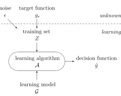
The machine conquers the task with a learning algorithm A. Generally speaking, the algorithm takes the learning model G and the training set Z as inputs. It then returns a decision function ˆg ∈ G by minimizing a predefined objective function E(g, Z) over g ∈ G. The full scenario of learning is illustrated in Figure 1.1.
Let us take one step back and look at what we mean by g∗ being the “best”
function to predicty fromx. To evaluate the predicting ability of any g: X → Y, we define its out-of-sample cost
π(g, F) =
Z
x,y
C y, g(x)dF(x, y).
noise target function
ǫ g∗
@ @
R ?
unknown
learning training set
Z
?
learning algorithm decision function
A ˆg
'
&
$
%
-6
[image:15.612.192.449.82.286.2]learning model G
Figure 1.1: Illustration of the learning scenario .
function g∗ should satisfy
π(g∗, F)≤π(g, F) ∀g:X → Y .
One of such a g∗ can be defined by
g∗(x)≡argmin
k∈Y
Z
y
C y, kdF(y|x)
. (1.1)
In this thesis, we assume that such ag∗ exists with ties in argmin arbitrarily broken,
and denote π(g, F) by π(g) when F is clear from the context.
Recall that the task of supervised learning is to find some ˆg ∈ G that is almost as good asg∗ under dF(x, y). Sinceπ(g∗) is the lower bound, we desire π(ˆg) to be as
depends only on Z is called the in-sample cost
ν(g) =
N
X
i=1
C yn, g(xn)
· N1 .
Note thatν(g) can also be defined byπ(g, Zu) whereZudenotes a uniform distribution
over the training set Z. Because ν(g) is an unbiased estimate of π(g) for any given single g, many learning algorithms take ν(g) as a major component of E(g, Z).
A small ν(g), however, does not always imply a small π(g) (Abu-Mostafa 1989; Vapnik 1995). When the decision function ˆg comes with a smallν(ˆg) and a largeπ(ˆg), we say that ˆg (or the learning algorithmA) overfits the training set Z. For instance, consider a training setZ withxn 6=xm for alln6=m, andC(y, k) = |y−k|. Assume
that a
ˆ g(x) =
yn, for x∈ {xn}Nn=1; some constant ∆, otherwise.
Then, we see that ν(ˆg) = 0 (the smallest possible value) and π(ˆg) can be as large as we want by varying the constant. That is, there exists a decision function like ˆg that leads to serious overfitting. Preventing overfitting is one of the most important objective when designing learning models and algorithms. Generally speaking, the objective can be achieved when the complexity of G (and hence the chosen ˆg) is reasonably controlled (Abu-Mostafa 1989; Abu-Mostafa et al. 2004; Vapnik 1995).
One important type of supervised learning problem is (univariate) regression, which deals with the case when Y is a metric space isometric to R. For simplic-ity, we shall restrict ourselves to the case where Y = R. Although not strictly re-quired, common regression algorithms usually not only work on someG that contains continuous functions, but also desires ˆg to be reasonably smooth as a control of its complexity (Hastie, Tibshirani and Friedman 2001). The metric information is thus important in determining the smoothness of the function.
squared cost. With the cost in mind, the ridge regression algorithm (Hastie, Tibshirani
and Friedman 2001) works on a linear regression model
G ={gv,b: gv,b(x) =hv,xi+b},
with ˆg being the optimal solution of
min
g∈G E(g, Z),
where E(gv,b, Z) =
λ
2hv,vi+ 1 N
N
X
n=1 Cs
yn, gv,b(xn)
.
The first part ofE(g, Z) controls the smoothness of the decision function chosen, and the second part is ν(gv,b).
Another important type of supervised learning problem is called classification, in whichY is a finite set Yc ={1,2, . . . , K}. Each label inYc represents a different
cate-gory. For instance, the digit recognition system described earlier can be formulated as a classification problem. A function of the formX → Yc is called a classifier. In the
special case where |Yc| = 2, the classification problem is called binary classification,
in which the classifier g is called a binary classifier.
To evaluate whether a classifier predicts the desired category correctly, a com-monly used cost function is the classification cost Cc(y, k) = Jy 6=kK.1 In some
classification problems, however, it may be desired to treat different kinds of clas-sification mistakes differently (Margineantu 2001). For instance, when designing a system to classify cells as {cancerous,noncancerous}, in terms of the possible loss on human life, the cost of classifying some cancerous cell as a noncancerous one should be significantly higher than the other way around. These classification problems would thus include cost functions other than Cc. We call them cost-sensitive classification
problems to distinguish them from the regular classification problems, which uses only Cc.
1
Note that in classification problems, for any given (x, y), the cost function C would be evaluated only on parameters (y, k) where k ∈ Yc. We can then represent
the needed part of C by a cost vector c with respect to y, where c[k] = C(y, k). In this thesis, we take a more general setup of cost-sensitive classification and allow dif-ferent cost functions to be used on difdif-ferent examples (Abe, Zadrozny and Langford 2004). In the setup, we assume that the vectorcis drawn from some probability mea-suredF(c|x, y) on a collectionC of possible cost functions. We call the tuple (x, y,c) the cost-sensitive example to distinguish it from a regular example (x, y). The learn-ing algorithm now receives a cost-sensitive trainlearn-ing set{(xn, yn,cn)}Nn=1to work with.2 Using the cost-sensitive examples (x, y,c), the out-of-sample cost becomes
π(g) =
Z
x,y
Z
c
c[g(x)] dF(c|x, y)
dF(x, y) ,
and the in-sample cost becomes
ν(g) =
N
X
i=1
cn[g(xn)]·
1 N .
As can be seen from the updated definitions of π(g) and ν(g), our setup do not explicitly need the label y. We shall, however, keep the notation for clarity and assume that y= argmin
k∈Y
c[k].
A special instance of cost-sensitive classification takes the cost vectorcto be of the formc[k] =w·Cc(y, k) for every cost-sensitive example (x, y,c) with somew≥0. We
call the instanceweighted classification, in which a cost-sensitive example (x, y,c) can be simplified to aweighted example (x, y, w). It is known that weighted classification problems can be readily solved by regular classification algorithms with rejection-based sampling (Zadrozny, Langford and Abe 2003).
2
1.2
Ordinal Ranking
Ordinal ranking is another type of supervised learning problem. It is similar to classification in the sense that Y is a finite set Yr = {1,2, . . . , K} = Yc. Therefore,
ordinal ranking is also calledordinal classification (Cardoso and da Costa 2007; Frank and Hall 2001). Nevertheless, in addition to representing the nominal categories (as the usual classification labels), now those y∈ Yr also carry the ordinal information.
That is, two different labels in Yr can be compared by the usual “<” operation. We
call thoseytheranks to distinguish them from the usual classification labels. We use aranker r(x) to denote a function from X → Yr. In an ordinal ranking problem, the
decision function is denoted by ˆr(x), and the target function is denoted by r∗(x).
Because ranks can be naturally used to represent human preferences, ordinal rank-ing lends itself to many applications in social science, psychology, and information retrieval. For instance, we may want to build a recommendation system that predicts how much a user likes a movie. We can first choose N movies and represent each movie by a feature vector xn. We then ask the user to (see and) rate each movie by
{one star, two star,. . ., five star}, depending on how much she or he likes the movie. The set Yr = {1,2, . . . ,5} includes different levels of preference (numbers of stars),
which are ordered by “<” to represent “worse than.” The task of this learning prob-lem is to set up an automatic recommendation system (decision function) ˆr: X → Yr
that is almost as good as the user, even on the yet unseen movies in the future. Ordinal ranking is also similar to regression, in the sense that ordinal information is similarly encoded in y ∈ R. Therefore, ordinal ranking is also popularly called ordinal regression (Chu and Ghahramani 2005; Chu and Keerthi 2007; Herbrich, Graepel and Obermayer 2000; Li and Lin 2007b; Lin and Li 2006; Shashua and Levin 2003; Xia, Tao, et al. 2007; Xia, Zhou, et al. 2007). Nevertheless, unlike the real-valued regression labels, the discrete ranks y ∈ Yr do not carry metric information.
many regression algorithms, and hence they may not perform well on ordinal ranking problems.
The ordinal information carried by the ranks introduce the following two proper-ties, which are important for modeling ordinal ranking problems.
• Closeness in the rank space Yr: The ordinal information suggests that the
mislabeling cost depend on the “closeness” of the prediction. For example, predicting a two-star movie as a three-star one is less costly than predicting it as a five-star one. Hence, the cost vector c should be V-shaped with respect toy (Li and Lin 2007b), that is,
c[k−1]≥c[k], for 2≤k ≤y;
c[k+1]≥c[k], fory ≤k ≤K−1.
(1.2)
Briefly speaking, a V-shaped cost vector says that a ranker needs to pay more if its prediction onxis further away fromy. We shall assume that every cost vec-tor c generated from dF(c|x, y) is V-shaped with respect to y = argmin
1≤k≤K
c[k]. With this assumption, ordinal ranking can be casted as a cost-sensitive classi-fication problem with V-shaped cost vectors.
In some of our results, we need a stronger condition: The cost vectors should be convex (Li and Lin 2007b), that is,
c[k+1]−c[k]≥c[k]−c[k−1], for 2≤k≤K−1. (1.3)
When using convex cost vectors, a ranker needs to pay increasingly more if its prediction on x is further away from y. It is not hard to see that any convex cost vector c is V-shaped with respect to y= argmin
1≤k≤K
c[k].
• Structure in the feature space X: Note that the classification cost vec-torsnc(cℓ): cc(ℓ)[k] =Jℓ6=kK
oK
what distinguishes ordinal ranking and regular classification?
Note that the total order withinYrand the target functionr∗introduces a total
preorder in X (Herbrich, Graepel and Obermayer 2000). That is,
x <∼x′ ⇐⇒r∗(x)≤r∗(x′).
The total preorder allows us to naturally group and compare vectors in the feature space X. For instance, a two-star movie is “worse than” a three-star one, which is in term “worse than” a four-star one; movies of less than three stars are “worse than” movies of at least three stars.
It is themeaningfulness of the grouping and the comparison that distinguishes ordinal ranking from regular classification, even when the classification cost vectors nc(cℓ)
oK
ℓ=1 are used. For instance, if apple = 1, banana = 2, grape = 3, orange = 4, strawberry = 5, we can intuitively see that comparing fruits {1,2} with fruits{3,4,5}is not as meaningful as comparing “movies of less than three stars” with “movies of at least three stars.”
There are some other algorithms that do not lead to such a quadratic expansion, such as perceptron ranking (Crammer and Singer 2005, PRank), ordinal regression boosting (Lin and Li 2006, ORBoost, which will be further introduced in Chapter 3), support vector ordinal regression (Chu and Keerthi 2007, SVOR), and the data repli-cation method (Cardoso and da Costa 2007). As we shall see later in Chapter 4, these algorithms can be unified under a simple reduction framework (Li and Lin 2007b).
Still some other algorithms fall into neither of the approaches above, such as C4.5-ORD (Frank and Hall 2001), Gaussian process ordinal regression (Chu and Ghahramani 2005, GPOR), recursive feature extraction (Xia, Tao, et al. 2007), and Weighted-LogitBoost (Xia, Zhou, et al. 2007).
1.3
Overview
In Chapter 2, we study the ordinal ranking problem from a classification perspec-tive. That is, we cast ordinal ranking as a cost-sensitive classification problem with V-shaped costs. We propose the cost-transformation technique to systematically ex-tend regular classification algorithms to their cost-sensitive versions. The technique carries strong theoretical guarantees. Based on the technique, we derive two novel cost-sensitive classification algorithms based on their popular versions in regular clas-sification and test their performance on both cost-sensitive clasclas-sification and ordinal ranking problems.
In Chapter 3, we study the ordinal ranking problem from a regression perspective. That is, we solve ordinal ranking by thresholding an estimation of a latent contin-uous variable. Learning models associated with this approach are called threshold models. We propose an novel instance of the threshold model called the threshold ensemble model and prove its theoretical properties. We not only extend RankBoost for constructing threshold ensemble rankers, but also propose a more efficient al-gorithm called ORBoost. The proposed alal-gorithm roots from the famous adaptive boosting (AdaBoost) approach and carries promising properties from its ancestor.
theoretically and algorithmically, which includes the threshold model as a special case. We derive theoretical foundations of the reduction framework and demonstrate a surprising equivalence: Ordinal ranking is as hard (easy) as binary classification. In addition to extending support vector machines (SVM) to ordinal ranking with the reduction framework, we also propose a novel algorithm called AdaBoost.OR, which efficiently constructs an ensemble of ordinal rankers as its decision function.
In Chapter 5, we include two concrete research projects that aim at understanding and improving binary classification. The results can in turn be coupled with the re-duction framework to improve ordinal ranking. First, we propose a novel framework of infinite ensemble learning based on SVM. The framework is not limited by the finiteness restriction of existing ensemble learning algorithms. Using the framework, we show that binary classification (and hence ordinal ranking) can be improved by going from a finite ensemble to an infinite one. Second, we discuss how AdaBoost carries the property of being resistant to overfitting. We then propose the Seed-Boost algorithm, which uses the property as a machinery to prevent other learning algorithms from overfitting.
Chapter 2
Ordinal Ranking by Cost-Sensitive
Classification
As discussed in Section 1.2, ordinal ranking can be casted as a cost-sensitive classifica-tion problem with V-shaped cost vectors. In this chapter, we study the cost-sensitive classification problem in general and propose a systematic technique to transform it to a regular classification problem. We first derive the theoretical foundations of the technique. Then, we use the technique to extend two popular algorithms for reg-ular classification, namely one-versus-one and one-versus-all, to their cost-sensitive versions. We empirically demonstrate the usefulness of the new cost-sensitive algo-rithms on general cost-sensitive classification problems as well as on ordinal ranking problems.
2.1
Cost-Sensitive Classification
For manipulating the training examples, Domingos (1999) proposed the MetaCost algorithm, which takes any classification algorithm to estimate dF(y|x), uses the estimate to relabel the training examples, and then retrains a classifier with the relabeled examples. The algorithm, however, depends strongly on how well dF(y|x) is estimated, which is hard to be theoretically guaranteed. In addition, the algorithm needs to know the cost collectionC in advance and only accepts some restricted forms ofdF(c|x, y). These shortcomings make it difficult to use the algorithm on our more general cost-sensitive setup. Approaches that manipulate the decision function suffer from similar shortcomings (Abe, Zadrozny and Langford 2004; Margineantu 2001).
There are many cost-sensitive classification approaches that come from modifying some regular classification algorithm (see, for instance, Margineantu 2001, Subsec-tion 2.3.2). These approaches are usually constructed by identifying where the clas-sification cost vectors are used in E(g, Z) (or some intermediate quantity within A), and then replacing them with cost-sensitive ones. Nevertheless, the modifications are usually ad hoc and heuristic based. In other words, those approaches usually do not come with a strong theoretical guarantee, either.
Recently, some authors proposed new algorithms for solving cost-sensitive classifi-cation problems directly (Beygelzimer et al. 2005; Beygelzimer, Langford and Raviku-mar 2007; Langford and Beygelzimer 2005). These algorithms come with stronger theoretical guarantee, but because of their novelty, they have not been as widely tested nor as successful as some popular algorithms for regular classification.
2.2
Cost-Transformation Technique
The key of the cost-transformation technique is to decompose a cost vector c to a conic combination of the classification cost vectors nc(cℓ)
oK
ℓ=1, where
c(cℓ)[k] =Cc(ℓ, k) =Jℓ 6=kK.
For instance, consider a cost vector ˜c= (4,3,2,3), we see that
˜
c= 0·(0,1,1,1)
| {z }
c(1)c
+1·(1,0,1,1)
| {z }
c(2)c
+2·(1,1,0,1)
| {z }
c(3)c
+1·(1,1,1,0)
| {z }
c(4)c .
Why is such a decomposition useful? If there is a cost-sensitive example (x, y,c), where c=PKℓ=1q˜[ℓ]·c(cℓ), then for any classifier g,
c[g(x)] =
K
X
ℓ=1 ˜
q[ℓ]·c(ℓ)
c [g(x)] = K
X
ℓ=1 ˜
q[ℓ]·Jℓ 6=g(x)K.
That is, if we sample ℓ proportional to ˜q[ℓ] and replace the cost-sensitive exam-ple (x, y,c) by a regular one (x, ℓ), then the cost thatg needs to pay for its prediction onxis proportional to the expected classification cost. Thus, if a classifierg performs well on the “relabeled” problem using the expected classification cost, it would also perform well on the original cost-sensitive problem. The nonnegativity of ˜q[ℓ] ensures that ˜q can be scaled to form a probability distributiondF(ℓ|q˜).1
Nevertheless, can every cost vector c be decomposed to a conic combination of nc(cℓ)
oK
ℓ=1? The short answer is no. For instance, the cost vector c = (2,1,0,1) cannot be decomposed to any conic combination of nc(cℓ)
o4
ℓ=1, because c comes with a unique linear decomposition:
(2,1,0,1) =−2
3 ·(0,1,1,1) + 1
3 ·(1,0,1,1) + 4
3·(1,1,0,1) + 1
3 ·(1,1,1,0).
1
Thus, c cannot be represented by any conic combination of nc(cℓ)
o4
ℓ=1. The unique existence of a linear combination is formalized in the following lemma.
Lemma 2.1. Any c ∈ RK can be uniquely decomposed to c = PℓK=1q[ℓ] · c(cℓ),
where q[ℓ]∈R for ℓ = 1,2, . . . , K.
Proof. Note thatq[ℓ] needs to satisfy the following matrix equation:
c[1] c[2] . . . c[K] | {z }
cT =
0 1 1 . . . 1 1 0 1 . . . 1 . . . .
1 1 1 . . . 0
| {z }
M q[1] q[2] . . . q[K] | {z }
qT .
Because M is invertible with
M−1 = 1 K−1
−(K−2) 1 1 . . . 1
1 −(K−2) 1 . . . 1 . . . .
1 1 1 . . . −(K−2)
,
the vector qcan be uniquely computed by M−1cTT. That is,
q[ℓ] = 1 K−1
K
X
k=1
c[k]
!
−c[ℓ].
Although ˜c = (4,3,2,3) yields a conic decomposition but c = (2,1,0,1) does not, the two cost vectors are not very different when being used to evaluate the performance of a classifier g. Note that for every x, ˜c[g(x)] = c[g(x)] + 2. The constant shifting from c to ˜c does not affect the relative cost difference between the prediction g(x) and the best prediction y. That is, using ˜c is equivalent to using c
when
˜
c[·] =c[·] + ∆,
with some constant ∆. If we only use c additively, as what we did in the definition of π(g) andν(g), using ˜cinstead of c would introduce only a constant shift.
Although we cannot decompose any c to a conic combination of nc(cℓ)
oK
ℓ=1, there exists infinitely many cost vectors ˜cthat allow a conic combination while being similar toc. To see this, note that
(K−1)·(∆,∆, . . . ,∆) = ∆
K
X
ℓ=1
c(cℓ).
Then, consider c=PKℓ=1q[ℓ]·c(cℓ),
˜
c=c+ (K−1)·(∆,∆, . . . ,∆) =
K
X
ℓ=1
(q[ℓ] + ∆)·c(cℓ).
We can easily make ˜q[ℓ] = q[ℓ] + ∆ ≥0 by choosing ∆≥ max
1≤ℓ≤K(−q[ℓ]).
Lemma 2.2. Consider some c=PKℓ=1q[ℓ]·cc(ℓ). If ˜c is similar to c by (K−1)·∆,
then ˜c yields a conic combination of nc(cℓ)
oK
ℓ=1 if and only if ∆≥1max≤ℓ≤K(−q[ℓ]).
Proof. By Lemma 2.1, the decomposition of ˜c by
K
X
ℓ=1
(q[ℓ] + ∆)·c(cℓ)
is unique. Then, it is not hard to see that ˜q[ℓ] =q[ℓ]+∆≥0 for everyℓ= 1,2, . . . , K if and only if ∆≥ max
1≤ℓ≤K(−q[ℓ]).
Lemma 2.2, there are infinitely many ˜cthat we can use. The next question is, which is more preferable? Since the proposed procedure relabels with probability
dF(ℓ|c) = ˜p[ℓ] = PKq˜[ℓ]
k=1q˜[k] ,
we would naturally desire the discrete probability distribution ˜p[·] to be of the least entropy. That is, we want the distribution to come from the optimal solution of
min ˜
p,∆
K
X
ℓ=1 ˜
p[ℓ] log 1 ˜
p[ℓ] , (2.1)
subject to ∆ ≥ max
1≤ℓ≤K(−q[ℓ]) ,
˜
p[ℓ] = PKq˜[ℓ]
k=1q˜[k]
, ℓ= 1,2, . . . , K, ˜
q[ℓ] = q[ℓ] + ∆, ℓ= 1,2, . . . , K,
q[ℓ] = 1
K−1
K
X
k=1
c[k]
!
−c[ℓ] , ℓ = 1,2, . . . , K.
Theorem 2.3. If not all c[ℓ] are equal, the unique optimal solution to (2.1) is
˜
p[ℓ] = PKcmax−c[ℓ]
k=1(cmax−c[k])
and ∆ = max
1≤ℓ≤K(−q[ℓ]), where cmax= max1≤ℓ≤Kc[ℓ].
Proof. If not all c[ℓ] are equal, not all q[ℓ] are equal. Now we substitute those ˜p in the objective function by the right-hand sides of the equality constraints. Then, the objective function becomes
f(∆) = −
K
X
ℓ=1
q[ℓ] + ∆
PK
k=1q[k] +K∆
logPKq[ℓ] + ∆
k=1q[k] +K∆ .
The constraint on ∆ ensures that all the plogp operations above are well defined.2
2
Now, let ¯q ≡ 1
K
PK
k=1q[k]. We get df
d∆ = −
1 K(¯q+ ∆)2
K
X
ℓ=1
(−q[ℓ] + ¯q)·
log
q[ℓ] + ∆ ¯ q+ ∆
−logK+ 1
= − 1
K(¯q+ ∆)2
K
X
ℓ=1
−(q[ℓ] + ∆) | {z }
aℓ
+ (¯q+ ∆)
| {z }
bℓ
·log q[ℓ] + ∆
¯ q+ ∆
= 1
K(¯q+ ∆)2
K
X
ℓ=1
aℓ−bℓ
· logaℓ−logbℓ
.
When not all q[ℓ] are equal, there exists at least one aℓ that is not equal to bℓ.
Therefore, ddf∆ is strictly positive, and hence the unique minimum of f(∆) happens when ∆ is of the smallest possible value. That is, for the unique optimal solution,
∆ = max
1≤ℓ≤K(−q[ℓ]) =cmax−
1
K−1
PK k=1c[k]
; ˜
q[ℓ] =cmax−c[ℓ], p˜[ℓ] = cmax−c[ℓ] PK
k=1(cmax−c[k]).
(2.2)
Using Theorem 2.3, we can define the following probability measure dFc(x, ℓ)
fromdF(x, y,c):
dFc(x, ℓ)∝
Z
y,c
˜
q[ℓ] dF(x, y,c),
where ˜q[ℓ] is computed from c using (2.2).3 More precisely, let
Λ1 = Z x,y,c K X ℓ=1 ˜
q[ℓ] dF(x, y,c). (2.3)
Note that from (2.2), PKℓ=1q˜[ℓ]>0 if not all c[ℓ] are equal. Thus, we can generally
3
assume that the integral results in a nonzero value. That is, Λ1 >0, and
dFc(x, ℓ) = Λ−11·
Z
y,c
˜
q[ℓ] dF(x, y,c).
Then, we can derive the following cost-transformation theorem:
Theorem 2.4. For any classifier g,
π(g, F) = Λ1·π(g, Fc)−Λ2,
where Λ2 = (K−1)·Rx,y,c∆·dF(x, y,c)and each∆in the integral is computed from c
with (2.2). Proof.
π(g, F) =
Z
x
Z
y,c
c[g(x)] dF(y,c|x)
dF(x)
= Z x Z y,c K X ℓ=1
q[ℓ]·c(cℓ)[g(x)] dF(y,c|x)
!
dF(x)
= Z x Z y,c K X ℓ=1
(˜q[ℓ]−∆)·cc(ℓ)[g(x)] dF(y,c|x)
!
dF(x)
= −Λ2+
Z x Z y,c K X ℓ=1 ˜
q[ℓ]·c(cℓ)[g(x)] dF(y,c|x)
!
dF(x)
= −Λ2+
Z
x K
X
ℓ=1
c(cℓ)[g(x)]·
Z
y,c
˜
q[ℓ] dF(y,c|x)
dF(x)
= −Λ2+ Λ1·
Z
x,ℓ
c(cℓ)[g(x)]·dFc(x, ℓ)
= −Λ2+ Λ1·π(g, Fc).
An immediate corollary of Theorem 2.4 is:
Corollary 2.5. If g∗ is the target function under dF(x, y,c), and g˜∗ is the target
function under dFc(x, ℓ), then π(g∗, F) =π( ˜g∗, F) and π(g∗, Fc) = π( ˜g∗, Fc).
func-tion ˆg = ˜g∗, the decision function is as good as the target function g∗ under the
original dF(x, y,c). Furthermore, as formalized in the following regret transforma-tion theorem, if any classifier g is close to ˜g∗ under dFc(x, ℓ), it is also close to g∗
under dF(x, y,c).
Theorem 2.6. ConsiderdFc(x, ℓ)defined fromdF(x, y,c)above, for any classifierg,
π(g, F)−π(g∗, F) = Λ1·
π(g, Fc)−π( ˜g∗, Fc)
.
Thus, to deal with a cost-sensitive classification problem generated fromdF(x, y,c), it seems that the learning algorithm A can take the following steps:
Algorithm 2.1 (Cost transformation with relabeling, preliminary).
1. ComputedFc(x, ℓ)and obtainN independent training examplesZc ={(xn, ℓn)}Nn=1 from dFc(x, ℓ).
2. Use a regular classification algorithm Ac on Zc to obtain a decision functiongˆc
that ideally yields a small π(ˆgc, Fc).
3. Return ˆg ≡ˆgc.
There is, however, a caveat in the algorithm above. Recall that dF(x, y,c) is unknown, and dFc(x, ℓ) depends on dF(x, y,c). Thus, dFc(x, ℓ) cannot be actually
computed. Nevertheless, we know that the training setZ ={(xn, yn,cn)}Nn=1contains
examples that are generated independently fromdF(x, y,c). Then, the first step can be implemented (almost equivalently) as follows.
Algorithm 2.2 (Cost transformation with relabeling).
1. Obtain N′ independent training examples Z
c ={(xn, ℓn)}N
′
n=1 from dFc(x, ℓ): (a) Transform each (xn, yn,cn) to (xn,q˜n) by (2.2).
(b) Apply the rejection-based sampling technique (Zadrozny, Langford and Abe
(c) For those (xn,˜qn) that survive from rejection-based sampling, randomly
assign its label ℓn with probabilityp˜n[ℓ]∝q˜n[ℓ].
2. Use a regular classification algorithm Ac on Zc to obtain a decision functiongˆc
that ideally yields a small π(ˆgc, Fc).
3. Return ˆg ≡ˆgc.
It is easy to check that the new training set Zc contains N′ (usually less than N)
independent examples from dFc(x, ℓ).
While the steps above are supported with theoretical guarantees from Theo-rems 2.4 and 2.6, they may not work well in practice. For instance, if we look at an example (xn, yn,cn) with yn = 1 and cn = (0,1,1,334), the resulting ˜qn =
(334,333,333,0). Because of the large value in cn[4], the example looks almost like a
uniform mixture of labels {1,2,3}, with only 0.334 of probability to keep its original label. In other words, for the purpose of encoding some large components in a cost vector, the relabeling process could pay a huge variance and relabel (or mislabel) the example more often than not. Then, the regular classification algorithmAc would
re-ceive someZcthat contains lots of misleading labels, making it hard for the algorithm
to return a decent ˆgc.
One remedy to the difficulty above is to use the following algorithm, calledtraining set expansion and weighting (TSEW), instead of relabeling:
Algorithm 2.3 (TSEW: training set expansion and weighting).
1. Obtain NK weighted training examples Zw ={(xnℓ, ynℓ, wnℓ)}:
(a) Transform each (xn, yn,cn) to (xn,q˜n) by (2.2).
(b) For every1≤ℓ≤K, let(xnℓ, ynℓ, wnℓ) = (xn, ℓ,q˜n[ℓ])and add(xnℓ, ynℓ, wnℓ)
to Zw.
2. Use a weighted classification algorithm Aw on Zw to obtain a decision
func-tion gˆw.
It is not hard to show that dFc(x, ℓ) ∝ w·dFw(x, ℓ, w), and Zw contains
(depen-dent) examples generated from dFw(x, ℓ, w). We can think of Zw, which trades
independence for smaller variance, as a more stable version of Zc. The expanded
training set Zw contains all possible ℓ, and hence always includes the correct
la-bel yn (along with the largest weight on ˜qn[yn]). The Aw in TSEW can also be
performed by a regular classification algorithm Ac using the rejection-based
sam-pling technique (Zadrozny, Langford and Abe 2003). Then, Algorithm 2.2 is simply a special (and less-stable) case of TSEW.
The TSEW algorithm is a basic instance of our proposed cost-transformation tech-nique. It is the same as the data space expansion (DSE) algorithm (Abe, Zadrozny and Langford 2004). Nevertheless, our derivation from the minimum entropy per-spective is novel, and our theoretical results on the out-of-sample cost π(g) are more general than the in-sample cost analysis by Abe, Zadrozny and Langford (2004). Re-cently, Xia, Zhou, et al. (2007) also proposed an algorithm similar to TSEW using LogitBoost as Aw based on a restricted version of Theorem 2.4. It should be noted
that the results discussed in this section are partially influenced by the work of Abe, Zadrozny and Langford (2004) but are independent from the work of Xia, Zhou, et al. (2007).
From the experimental results, TSEW (DSE) does not perform well in prac-tice (Abe, Zadrozny and Langford 2004). A possible reason is that common Aw
still findZw too difficult (Xia, Zhou, et al. 2007), because a training feature vectorxn
could be multilabeled in Zw, which may confuse Aw. One could improve the basic
TSEW algorithm by using (or designing) anAwthat is more robust with multilabeled
training feature vectors, as discussed in the next section.
2.3
Algorithms
2.3.1
Cost-Sensitive One-Versus-All
Theone-versus-all (OVA) algorithm is a popular algorithm for weighted classification. It solves the weighted classification problem by decomposing it to several weighted binary classification problems, as shown below.
Algorithm 2.4 (One-versus-all, see, for instance, Hsu and Lin 2002).
1. For each 1≤ℓ≤K,
(a) Take the original training set Z ={(xn, yn, wn)}Nn=1 and construct a binary
classification training set Zb(ℓ) =n(xn, yn(ℓ), wn) : yn(ℓ) =Jyn =ℓK
oN n=1. (b) Use a weighted binary classification algorithm Ab on Zb(ℓ) to get a decision
function ˆgb(ℓ).
2. Return ˆg(x) = argmax 1≤ℓ≤K
ˆ gb(ℓ)(x).
Each ˆgb(ℓ)(x) intends to predict whether x belongs to category ℓ. Thus, if a feature vectorxshould be of category 1, and all ˆgb(ℓ) are mistake free, then ideally ˆg(1)b (x) = 1 and ˆg(bℓ)(x) = 0 for ℓ 6= 1, and hence ˆg(x) could make a correct prediction. Never-theless, if some of the binary decision functions ˆgb(ℓ) make mistakes, the performance of OVA can be affected by the ties in the argmax operation. In practice, the OVA algorithm usually allows the decision functions ˆgb(ℓ) to output a soft prediction (say, in [0,1]) rather than a hard one of {0,1}. The soft prediction represents the sup-port (confidence) on whetherxbelongs to categoryℓ, and ˆg(x) returns the prediction associated with the highest support.
What would happen if we directly use OVA as Aw in TSEW? Recall that a
cost-sensitive training example x1,1,(0,1,1,334) in Z would introduce the following multilabeled examples in Zw:
If we feedZw directly to OVA, the underlying binary classification algorithmAb would
use the following examples to get ˆg(1)b :
(x1,1,334),(x1,0,666).
That is, even thoughx1 is of category 1, paradoxically we preferAb to return some ˆgb(1)
that predicts x1 as 0 rather than 1. The paradox is similar to what we encountered when sampling Zc from Z in Algorithm 2.1: The relabeling process results in a
misleading label more often than not. Thus, directly plugging OVA into the TSEW algorithm does not work.
Nevertheless, we can modify OVA and make it more robust when given multi-labeled training examples. In fact, a variant of the OVA algorithm can readily be used for multilabeled classification in literature (see, for instance, Joachims 2005, Section 2). For a training feature vector xn that can be labeled either as 1 or 2, the
OVA algorithm for a multilabeled training set Z would pair xn with y(1)n = 1 when
constructing Zb(1), and with yn(2) = 1 when constructingZb(2) as well. That is, when Z
contains both (and only) (xn,1) and (xn,2), the feature vector xn “supports” both
category 1 and 2, while it does not support categories 3, 4,. . ., K.
The support perspective can also be understood with the cost vectors and the cost-transformation technique. Note that the expanded training set Zw contains
both (xn,1) and (xn,2) (with weights 1) if and only if the original cost-sensitive
train-ing example (xn, yn,cn) comes with a cost vectorcnthat is similar to (0,0,1,1, . . . ,1).
Thus, xn supports both categories 1 and 2 because no cost needs to be paid when the
prediction falls in them. Note that ˜qn = (1,1,0,0, . . . ,0) in this case. Equivalently
speaking, we can say thatxn supports those categories ℓwith ˜qn[ℓ] = 1 and does not
From the observation above, we can defines[ℓ] = q˜q˜max[ℓ] as the support for categoryℓ, where ˜qmax = max1≤ℓ≤Kq˜[ℓ]. Thus,s[ℓ]∈[0,1], and from (2.2),
s[ℓ] = 0 when c[ℓ] =cmax,
s[ℓ] = 1 when c[ℓ] =cmin = min1≤k≤Kc[k].
With the definition above, we propose the generalized OVA algorithm, which takes the original OVA algorithm as a special case.
Algorithm 2.5 (Generalized one-versus-all).
1. For each 1 ≤ ℓ ≤ K, use Ab to learn a binary classifier ˆgb(ℓ)(x) with the hope
that
Z
x,y,c
˜ qmax·
s[ℓ]−ˆgb(ℓ)(x)2 dF(x, y,c) (2.4) is small.
2. Return ˆg(x) = argmax 1≤ℓ≤K
ˆ gb(ℓ)(x).
How can Ab learn a binary classifier? Equation (2.4) is deliberately
formu-lated as a learning problem. Then, for each training example (xn, yn,cn) obtained
from dF(x, y,c), we can compute a new training example (xn, yn,sn[ℓ],(˜qmax)n) to
provide information for solving such a learning problem. Assume that we keep the convention x(nℓ) = xn and yn(ℓ) = Jyn=ℓK in Algorithm 2.4 and try to approximately
deal with (2.4) by casting it as a weighted binary classification problem. One simple method to obtain the weight w(nℓ) from xn, yn,sn[ℓ],(˜qmax)n
is4
wn(ℓ) =
(˜qmax)n·sn[ℓ] when yn =ℓ ;
(˜qmax)n·(1−sn[ℓ]) when yn 6=ℓ .
(2.5)
4
By replacing step 1 of generalized OVA with the weighted binary classification prob-lem, we get thecost-sensitive one-versus-all (CSOVA) algorithm, as formalized below.
Algorithm 2.6 (CSOVA: Cost-sensitive one-versus-all).
1. For each 1≤ℓ≤K,
(a) Take the original training set Z ={(xn, yn,cn)}Nn=1 and construct a binary classification training set Zb(ℓ) =n(xn, yn(ℓ), w(nℓ))
o
from (2.5).
(b) Use a weighted binary classification algorithm Ab on Zb(ℓ) to get a decision
function ˆgb(ℓ).
2. Return ˆg(x) = argmax 1≤ℓ≤K
ˆ gb(ℓ)(x).
We can easily see Algorithm 2.4 is a special case of Algorithm 2.6 when all cn are
classification cost vectors.
2.3.2
Cost-Sensitive One-Versus-One
Theone-versus-one (OVO) algorithm is another popular algorithm for weighted clas-sification. It is suitable for practical use when K is not too large (Hsu and Lin 2002). Similar to the OVA algorithm, it also solves the weighted classification problem by decomposing it to several weighted binary classification problems. Unlike OVA, how-ever, each binary classification problem consists of comparing examples from two categories only.
Algorithm 2.7 (One-versus-one, see, for instance, Hsu and Lin 2002).
1. For each i, j that1≤i < j ≤K,
(a) Take the original training set Z ={(xn, yn, wn)}Nn=1 and construct a binary
classification training set Zb(i,j)={(xn, yn, wn) : yn=i or yn =j}.
(b) Use a weighted binary classification algorithmAb onZb(i,j) to get a decision
2. Return ˆg(x) = argmax 1≤ℓ≤K
P
i<j
r ˆ
gb(i,j)(x) =ℓz.
In short, each ˆgb(i,j)(x) intends to predict whether x“prefers” i or category j, and ˆg predicts with the preference votes gathered from those ˆgb(i,j). The goal of Ab is to
locate decision functions ˆgb(i,j) with a small πˆgb(i,j), F(i,j), where dF(i,j)(x, y) = dF(x, y|y=ior j), because it can be proved that (Beygelzimer et al. 2005)
π(ˆg)≤2X
i<j
Prob [y=ior j]·πgˆb(i,j), F(i,j).
Let us see if we can use OVO as Aw in TSEW for cost-sensitive classification
problems. Again, consider a cost-sensitive training example x1,1,(0,1,1,334)inZ. Recall that it would introduce the following multilabeled examples in Zw:
(x1,1,334),(x1,2,333),(x1,3,333).
If we directly use OVO as Aw in TSEW, the underlying binary classification
algo-rithm Ab would use the following two examples in Zb(1,2) to get ˆg
(1,2)
b :
(x1,1,334),(x1,2,333).
Note that these weighted examples can be equivalently generated by labeling x1 as 1 with probability 334
667 and as 2 with probability 333
667. Because the probabilities are both close to 1
2, the labels are almost as if decided by throwing a fair coin. Therefore, the binary classification algorithm Ab may be confused by the two examples.
For any classifier gb(i,j): X → {i, j}, and a given example (x1, y1,c1) above, we see that the classifier needs to pay a constant cost of 333 first, regardless of its prediction. Now, we can again use the technique of shifting costs by a constant as we did in constructing similar cost vectors. Then, the two examples (x1,1,334),(x1,2,333) is the same as one single example of (x1,1,1). The shifting not only simplifies Zb(i,j)
Recall that Zw consists of examples (xnℓ, ynℓ, wnℓ) = (xn, ℓ,q˜n[ℓ]). Thus, (xn, i)
would be of weight ˜qn[i] and (xn, j) would be of weight ˜qn[j]. By the discussion
above, the simplified Zb(i,j) consists of
Zb(i,j) =
xn,argmax ℓ=i orj
˜
qn[ℓ],
q˜n[i]−q˜n[j]
=
xn,argmin ℓ=i orj
cn[ℓ],
cn[i]−cn[j]
. (2.6)
Then, we get our proposed cost-sensitive one-versus-one (CSOVO) algorithm.
Algorithm 2.8 (CSOVO: Cost-sensitive one-versus-one).
1. For each i, j that1≤i < j ≤K,
(a) Take the original training set Z ={(xn, yn,cn)}Nn=1 and construct a binary classification training set by (2.6).
(b) Use a weighted binary classification algorithmAb onZb(i,j) to get a decision
function ˆgb(i,j).
2. Return ˆg(x) = argmax 1≤ℓ≤K
P
i<j
r ˆ
gb(i,j)(x) =ℓz.
We can easily see that CSOVO takes OVO as a special case when the using only the classification cost vectors. In addition, we can think of each created exam-ple
xn,argmin ℓ=i orj
cn[ℓ],
cn[i]−cn[j]
as if coming from a (possibly unnormalized) measure
dFb(i,j)(x, k, w) =
Z
y,c
s
k = argmin
ℓ=i orj
cn[ℓ]
{ r w=
c[i]−c[j]
z
dF(x, y,c).
Define
πb(i,j)(g(i,j)) =
Z
x,k,w
wqk 6=g(i,j)(x)y dFb(i,j)(x, k, w).
Theorem 2.7. For any family of classifiers ngb(i,j): 1≤i < j ≤Ko, where the bi-nary classifiers gb(i,j): X → {i, j}. Let
g(x) =argmax 1≤ℓ≤K
X
i<j
r
g(bi,j)(x) =ℓz.
Then,
π(g)−
Z
x,y,c
cmin dF(x, y,c)≤2
X
i<j
πb(i,j)g(bi,j).
Proof. For each (x, y,c) generated from dF(x, y,c), if c[g(x)] = c[y] = cmin, its contribution on the left-hand side is 0, which is trivially less than its contribution on the right-hand side.
Without loss of generality (by sorting the elements of the cost vector c and shuf-fling the labels y∈ Y), consider an example (x, y,c) such that
cmin=c[1]≤c[2]≤ . . .≤c[K] =cmax.
From the results of Beygelzimer et al. (2005, Lemma 1), suppose g(x) = k, then for each 1 ≤ ℓ ≤ k−1, there are at least ⌈k/2⌉ pairs (i, j), where i ≤ k < j, and argmin
ℓ=i or j
cn[ℓ]6=gb(i,j)(x). Therefore, the contribution of (x, y,c) on the right-hand side
is no less than
k−1
X
ℓ=1
(c[ℓ+ 1]−c[ℓ])
ℓ 2 ≥ 1 2
k−1
X
ℓ=1
ℓ(c[ℓ+ 1]−c[ℓ])
= 1
2
k
X
ℓ=2
(ℓ−1)c[ℓ]− 1 2
k−1
X
ℓ=1 ℓc[ℓ]
= 1
2(k−1)c[k]− 1 2
k−1
X
ℓ=1
c[ℓ]
= 1
2
k−1
X
ℓ=1
(c[k]−c[ℓ])
≥ 1
and the left-hand-side contribution is (c[k]−cmin). The desired result can be proved by integrating over alldF(x, y,c).
Theorem 2.7 provides a theoretical guarantee for CSOVO: If each ˆg(bi,j) yields a small πb(i,j), the resulting ˆg would yield a smallπ. Beygelzimer et al. (2005) proposed another algorithm, calledweighted all-pairs (WAP), that shared a similar theoretical guarantee and some algorithmic structures, as listed below.
Algorithm 2.9 (A special case of WAP, Beygelzimer et al. 2005).
1. For each i, j that1≤i < j ≤K,
(a) Take the original training set Z ={(xn, yn,cn)}Nn=1 and construct a binary
classification training set by
Zb(i,j) =
(
xn,argmin ℓ=i or j
cn[ℓ],
Z cn[i]
cn[j]
1
|{k: cn[k]≤t}|
dt !) (2.7)
(b) Use a weighted binary classification algorithmAb onZb(i,j) to get a decision
function ˆgb(i,j).
2. Return ˆg(x) = argmax 1≤ℓ≤K
P
i<j
r ˆ
gb(i,j)(x) =ℓz.
We see that WAP is similar to CSOVO (Algorithm 2.8), except for how the weights of the binary examples are computed. CSOVO uses
cn[i]−cn[j]
, which is equivalent
to
Z cn[i]
cn[j]
(1)dt .
Table 2.1: Classification data sets
data set # examples # categories (K) # features (D)
vehicle 846 4 18
vowel 990 11 10
segment 2310 7 19
dna 3186 3 180
satimage 6435 6 36
usps 9298 10 256
2.4
Experiments
In this section, we compare the proposed CSOVA and CSOVO algorithms derived from the cost-transformation technique with their original versions. We also compare CSOVO with its closely related sibling, the WAP algorithm. All these algorithms obtains a decision function ˆg by calling a binary classification algorithm Ab several
times. We take the support vector machine (SVM) with the perceptron kernel (Lin and Li 2008, which will be further introduced in Chapter 5) as Ab in all the
experi-ments and use LIBSVM (Chang and Lin 2001) as our SVM solver.
2.4.1
Comparison on Classification Data Sets
We first compare the algorithms with six benchmark classification data sets: vehicle,
vowel, segment, dna, satimage, usps (Table 2.1).5 The first five comes from the UCI machine learning repository (Hettich, Blake and Merz 1998) and the last one comes from Hull (1994).
The six data sets in Table 2.1 were originally gathered as regular classification problems. We adopt two kinds of setup to compare cost-sensitive algorithms. In the first one, called therandomized proportional (RP) cost setup, we follow the procedure used by Abe, Zadrozny and Langford (2004). In particular, we generate the cost vectors from a cost function C(y, k) that does not depends on x. C(y, y) is set as 0 and C(y, k) is a random variable sampled uniformly from h0,2000|{n:yn=k}|
|{n:yn=y}|
i
.
Another setup is the absolute cost setup, which considers the absolute cost
vec-5
tors nc(aℓ)
oK
ℓ=1 with
c(aℓ)[k] =Ca(ℓ, k) =|ℓ−k|.
Note that the absolute cost vectors are not only V-shaped but also convex, and they are widely used in evaluating ordinal ranking algorithms (Chu and Keerthi 2007; Li and Lin 2007b).
We randomly choose 75% of the examples in each data set for training and leave the other 25% of the examples as the test set. Then, each feature in the training set is linearly scaled to [−1,1], and the feature in the test set is scaled accordingly. The results reported are all averaged over 20 trials of different training/test splits, along with the standard error.
SVM with the perceptron kernel takes a regularization parameter (Lin and Li 2008), which is chosen within{2−17,2−15, . . . ,23} with a 5-fold cross-validation (CV) procedure on the training set (Hsu, Chang and Lin 2003). For the original OVA and OVO, the CV procedure selects the parameter that results in the smallest cross-validation regular classification cost. For the other algorithms, the CV procedure selects the parameter that results in the smallest cross-validation cost-sensitive clas-sification cost based on the given setup. We then rerun each algorithm on the whole training set with the chosen parameter to get the decision function ˆg. Finally, we evaluate the average performance of ˆg on the test set.
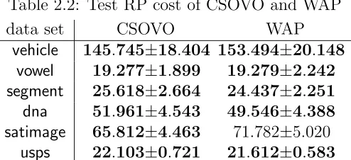
In Tables 2.2 and 2.3, we first compare CSOVO with WAP using the RP cost setup and the absolute cost setup, respectively. We see that the two algorithms perform similarly on almost all data sets. Because CSOVO is indistinguishable with WAP in terms of performance while enjoying an advantage of a simpler and more efficient implementation (see Subsection 2.3.2), it should be preferred in practice.
Table 2.2: Test RP cost of CSOVO and WAP
data set CSOVO WAP
vehicle 145.745±18.404 153.494±20.148 vowel 19.277±1.899 19.279±2.242 segment 25.618±2.664 24.437±2.251 dna 51.961±4.543 49.546±4.388 satimage 65.812±4.463 71.782±5.020
usps 22.103±0.721 21.612±0.583
(those within one standard error of the lowest one are marked in bold)
Table 2.3: Test absolute cost of CSOVO and WAP
data set CSOVO WAP
vehicle 0.225±0.007 0.225±0.007 vowel 0.030±0.005 0.031±0.004 segment 0.045±0.003 0.046±0.003 dna 0.067±0.002 0.066±0.002 satimage 0.127±0.003 0.128±0.003 usps 0.089±0.002 0.090±0.003
(those within one standard error of the lowest one are marked in bold)
algorithms.
Table 2.4: Test RP cost of cost-sensitive classification algorithms
data one-versus-all one-versus-one
set OVA CSOVA OVO CSOVO
vehicle 189.064±17.866 158.215±19.833 185.378±17.235 145.745±18.404 vowel 14.654±1.766 14.386±1.717 11.896±1.955 19.277±1.899
segment 25.263±2.015 25.434±2.208 25.153±2.109 25.618±2.664 dna 44.480±2.771 39.424±2.521 48.152±3.333 51.961±4.543
satimage 93.381±5.712 77.101±4.762 94.075±5.488 65.812±4.463 usps 23.087±0.709 22.793±0.710 23.622±0.660 22.103±0.721
(those within one standard error of the lowest one are marked in bold)
Table 2.5: Test absolute cost of cost-sensitive classification algorithms
data one-versus-all one-versus-one
set OVA CSOVA OVO CSOVO
vehicle 0.222±0.007 0.226±0.007 0.221±0.007 0.225±0.007 vowel 0.029±0.005 0.030±0.005 0.023±0.004 0.030±0.005
segment 0.042±0.003 0.043±0.003 0.041±0.003 0.045±0.003
dna 0.053±0.002 0.054±0.002 0.056±0.002 0.067±0.002
satimage 0.124±0.003 0.123±0.003 0.125±0.003 0.127±0.003
usps 0.077±0.002 0.077±0.002 0.080±0.002 0.089±0.002 (those within one standard error of the lowest one are marked in bold)
2.4.2
Comparison on Ordinal Ranking Data Sets
Next, we compare the algorithms with eight benchmark ordinal ranking data sets:
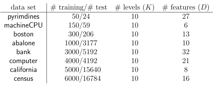
pyrimdines,machineCPU,boston,abalone,bank,computer,california,census(Table 2.6), which were used by Chu and Keerthi (2007). Similar to the original setup of Chu and Keerthi (2007), we kept the same training/test split ratios, used the absolute cost vectors for evaluating the performance and averaged the results over 20 trials.
[image:46.612.140.507.279.396.2]Table 2.6: Ordinal ranking data sets
data set # training/# test # levels (K) # features (D)
pyrimdines 50/24 10 27
machineCPU 150/59 10 6
boston 300/206 10 13
abalone 1000/3177 10 10
bank 3000/5192 10 32
computer 4000/4192 10 21
california 5000/15640 10 8
[image:47.612.137.508.295.441.2]census 6000/16784 10 16
Table 2.7: Test absolute cost of cost-sensitive classification algorithms on ordinal ranking data sets
data one-versus-all one-versus-one
set OVA CSOVA OVO CSOVO
pyrimdines 1.765±0.103 1.627±0.055 1.746±0.076 1.337±0.054 machineCPU 0.983±0.027 0.975±0.024 1.009±0.024 0.842±0.023 boston 0.987±0.019 0.946±0.017 0.882±0.017 0.789±0.015 abalone 1.719±0.007 1.674±0.007 1.632±0.013 1.422±0.006 bank 1.863±0.007 1.801±0.004 1.632±0.004 1.414±0.003 computer 0.685±0.003 0.644±0.003 0.620±0.002 0.575±0.002 california 1.164±0.004 1.121±0.002 1.055±0.003 0.951±0.002 census 1.381±0.004 1.329±0.003 1.272±0.002 1.135±0.001
(those within one standard error of the lowest one are marked in bold)
Chapter 3
Ordinal Ranking by Threshold
Regression
As discussed in Section 1.2, ordinal ranking is similar to regression because the labels in either Yrand Rrepresent ordinal information. Nevertheless, unlike the real-valued
regression labels in R, the discrete ranks in Yr do not carry metric information.
That is, ordinal ranking deals with qualitative, fuzzy ranks while regression focuses on quantitative, real-valued outcomes. To model ordinal ranking problems from a regression perspective, it is often assumed that some underlying real-valued outcomes exist, but are unobservable (McCullagh 1980). The hidden local scales “around” different ranks can be quite different, but the actual scale (metric) information is not encoded in the ranks.
Under the assumption above, each rank represents a contiguous interval on the real line. Then, ordinal ranking can be approached by the following abstract algorithm called threshold regression.
Algorithm 3.1 (Threshold regression).
1. Estimate a potential functionH(x)that predicts (a monotonic transform of ) the real-valued outcomes. Ideally, feature vectors of larger ranks should be associated
with larger potential values.
-d -d
θ1 t t tθ2 x xx xθ3 ++
1
2
3
4
rH,θ(x) [image:49.612.195.445.60.130.2]H(x)
Figure 3.1: Prediction procedure of a threshold ranker
In the threshold regression algorithm, the potential function intends to uncover the nature of the assumed underlying outcome, and the threshold vector estimates the possibly different scales around different ranks. The two abstract steps of the algorithm are indeed taken by many existing ordinal ranking algorithms. For instance, in the GPOR algorithm of Chu and Ghahramani (2005), the potential functionH(x) is assumed to follow a Gaussian process, and the threshold vector θ is determined by Bayesian inference with respect to some noise distribution. In the PRank algorithm of Crammer and Singer (2005), the potential function Hv is taken to be a linear
function of the form Hv(x) = hv,xi, and the pair (v, θ) are updated simultaneously.
Some other algorithms are based on SVM, and they work on potential functions of the form Hv(x) = hv, φ(x)i, where φ(x) maps x ∈ RD to some Hilbert space (Chu
and Keerthi 2007; Herbrich, Graepel and Obermayer 2000; Shashua and Levin 2003). The learning model associated with the threshold regression algorithm is called the threshold model. Formally speaking, the threshold model RP ={rH,θ}, where H ∈ P
and −∞=θ0 ≤ θ1 ≤θ2 ≤ . . .≤ θK−1 ≤θK = ∞. As illustrated in Figure 3.1, each
member rH,θ of the threshold model is athreshold ranker, which makes its prediction
by
rH,θ(x) = min{k: H(x)≤θk}= max{k: H(x)> θk−1}= 1 +
K−1
X
k=1
JH(x)> θkK.(3.1)
We denote rH,θ asrθ when H is clear from the context.
Section 3.1 and Chapter 4. Each ranker in the threshold ensemble model is called a threshold ensemble, which uses an ensembleHT of confidence functions as the potential
function H. The ensemble is of the form
HT(x) = T
X
t=1
αtht(x), αt∈R. (3.2)
We assume that each confidence functionht: X →[−1,+1] comes from a hypothesis
set H. That is, HT ∈ span(H) = P. The confidence function reflects a possibly
imperfect ordering preference. Note that a special instance of the confidence function is a binary classifierX → {−1,+1}, which matches the fact that binary classification is a special case of ordinal ranking with K = 2 (Rudin et al. 2005). The ensemble linearly combines the ordering preferences with α. Note that we allow αt to be any
real value, which means that it is possible to reverse the ordering preference of ht in
the ensemble when necessary.
Ensemble models in general have been successfully used for classification and re-gression (Meir and R¨atsch 2003). They not only introduce more stable predictions through the linear combination, but also provide sufficient power for approximating complicated target functions. The threshold ensemble model extends existing ensem-ble models to ordinal ranking and inherits many useful theoretical properties from them. Next, we discuss one such property: the large-margin bounds.
3.1
Large-Margin Bounds of Threshold Ensembles
The margin concept in binary classification says large margins produced by a binary classifiergshould indicate a small π(g). The concept is widely used to evaluate binary classifiers (Li et al. 2005; Vapnik 1995) and can be justified with many large-margin cost bounds of the form
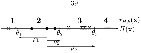
-d -d
θ1 t t tθ2 x xx xθ3 ++ ρ1 ρ2
-ρ3
1
2
3
4
rH,θ(x) [image:51.612.197.438.63.154.2]H(x)
Figure 3.2: Margins of a correctly predicted example
where ν(g,∆) = π(g, Zu,∆) is an extended form of training cost with respect to a
margin parameter ∆, and the complexity term decreases as N or ∆ increases. For ordinal ranking using threshold models, Herbrich, Graepel and Obermayer (2000) derived a large-margin bound for any threshold ranker rθ with a potential
function Hv = hv, φ(x)i. Unfortunately the bound is quite restricted since it is
only applicable when ν(rθ,∆) = 0 with respect to the classification cost function Cc.
In addition, the bound uses a margin definition that contains O(N2) terms, which makes it more complicated to design algorithms that relate to the bound. Another bound was derived by Shashua and Levin (2003). The bound is based on a margin definition of only O(KN) terms and is applicable to the threshold ensemble model. Nevertheless, the bound is loose when T, the size of the ensemble, is large, because its complexity term grows with T.
Next, we derive novel large-margin bounds of the threshold ensemble model with two widely used cost functions: the classification cost function Cc and the
abso-lute cost function Ca. Similar bounds for more general cost-sensitive setup will be
discussed in Chapter 4. The bounds are extended from the results of Schapire et al. (1998) and are based on a margin definition ofO(KN) terms. In addition, our bounds do not require ν(rθ,∆) = 0 with respect to Cc, and their complexity terms do not
grow withT.
Definition 3.1. Consider a given threshold ensemble rH,θ, where H =HT.
1. The margin of an example (x,