KVA: Capital Valuation Adjustment

KVA: Capital Valuation Adjustment

∗

Andrew Green

, Chris Kenyon

and Chris Dennis

February 20, 2014

Version 1.0

Abstract

Credit (CVA), Debit (DVA) and Funding Valuation Adjustments (FVA) are now familiar valuation adjustments made to the value of a portfolio of derivatives to account for credit risks and funding costs. However, recent changes in the regulatory regime and the increases in regulatory capital re-quirements has led many banks to include thecost of capital in derivative pricing. This paper formalises the addition of cost of capital by extending the Burgard-Kjaer (2013) semi-replication approach to CVA and FVA to include an addition capital term, Capital Valuation Adjustment (KVA).1 Two approaches are considered, one where the (regulatory) capital is re-leased back to shareholders upon counterparty default and one where the capital can be used to offset losses in the event of counterparty default. The use of the semi-replication approach means that the flexibility around the treatment of self-default is carried over into this analysis. The paper further considers the practical calculation of KVA with reference to the Basel II (BCBS-128 2006) and Basel III (BCBS-189 2011) Capital regimes and its implementation via CRD IV (EU 2013b; EU 2013a). The paper assesses how KVA may be hedged, given that any hedging transactions themselves would lead to regulatory capital requirements and hence KVA. To conclude, a number of numerical examples are presented to gauge the cost impact of KVA on vanilla derivative products.

1

Introduction

Capital is a legal requirement for financial institutions holding derivatives, and requirements have increased over the past few years (Dodd and Frank 2010; Department of the Treasury 2013; EU 2013b; EU 2013a). Hence it is surprising that few papers include capital in derivatives pricing, (Kenyon and Green 2013a; Kenyon and Green 2013b). Here we extend the hedging framework of (Burgard and Kjaer 2011; Kenyon and Kenyon 2013; Burgard and Kjaer 2013) to price capital requirements of derivatives trades by replicating its costs, together with

∗_{The views expressed are those of the authors only, no other representation}

should be attributed.

†_{Contact: [email protected]} ‡_{Contact: [email protected]} §_{Contact: [email protected]}

1_{i.e. Kapital Valuation Adjustment to distinguish from CVA.}

the costs from credit and funding. Thus we present a Capital Valuation Adjust-ment (KVA) alongside the existing adjustAdjust-ments for credit and funding.

Capital pricing appears challenging for several reasons:

1. Diversity and length of regulations (see below). In Basel III there are several major categories, each with hundreds of pages.

2. Lifetime capital costs are needed, not just the spot costs.

3. Calculations must be done at several different levels of granularity and combined. For example, for counterparty credit risk and CVA capital netting sets are important, while bank-level portfolio can also be needed such as for determination of the stressed period for Market Risk for SVAR calculation. Under the standardized approach CVA capital is calculated across all counterparties.2

4. The date when new regulation comes into force, and the exact content of them is often uncertain, for example a series of new regulations are currently in a consultation phase,fundamental review of the trading book

(BCBS-219 2012; BCBS-265 2013),NIMM (BCBS-254 2013),margin re-quirements for non-centrally cleared derivatives(BCBS-261 2013) and pru-dent valuation(EBA 2013).

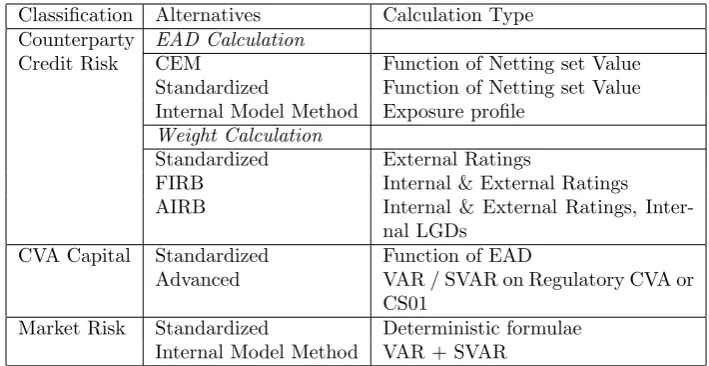
We present a brief list below of typical capital regulations here based on Basel III, and the type of calculation they require in Table 1.

Whilst capital calculation may appear challenging, these calculations do not at first seem to introduce anything fundamentally different from CVA or FVA calculation. The truly new element is handling the capital itself, that is, deciding what happens to the capital on counterparty default. There are two approaches here that we call Capital Allocation and Capital Insurance.

• Capital Allocation = the desk has been allocated the capital it pays for, but the desk takes no ownership: on counterparty default the capital is unaffected.

• Capital Insurance = the desk has bought insurance against unexpected risks by paying for capital: on counterparty default the first losses are born by the capital.

Since bank losses hit capital the second alternative appears more realistic, al-though in practice it will depend on the policy applied by individual banks. Overall, there are also new complexities when we consider the capital require-ments on the positions that we use to hedge the capital costs and this is explored in more detail in section 3 below. We deal with other, systematic, theoretical consequences elsewhere (Kenyon and Green 2013b).

The main contribution of this paper is to complete the pricing picture by including the costs of capital, the Capital Valuation Adjustment (KVA), in derivatives pricing by replication. Given the increased regulatory focus on cap-ital post-crisis, continuing regulatory developments, and its cost, this is long overdue.

2_{In practice for large numbers of counterparties it is well approximated by a summation}

over terms against individual counterparties as is described in section 4.3.1.

Classification Alternatives Calculation Type Counterparty EAD Calculation

Credit Risk CEM Function of Netting set Value Standardized Function of Netting set Value Internal Model Method Exposure profile

Weight Calculation

Standardized External Ratings

FIRB Internal & External Ratings AIRB Internal & External Ratings,

Inter-nal LGDs CVA Capital Standardized Function of EAD

Advanced VAR / SVAR on Regulatory CVA or CS01

Market Risk Standardized Deterministic formulae Internal Model Method VAR + SVAR

Table 1: Typical categories of capital regulations, their diversity (alternatives), and the type of calculations they require.

1.1

Diversity in Regulatory Capital Requirements

Different quantities of capital are required for the same portfolio depending on the institution’s regulatory status, and its interpretation of the regulations (BCBS-267 2013). The capital requirements also change depending on the inten-tion of the instituinten-tion, hold-to-maturity posiinten-tions (Banking Book) have different capital requirements to available-for-sale (Trading Book) (BCBS-265 2013). Our replication pricing is applicable to all these cases. This does however mean that different institutions will have different replication costs, we go into detail on the implications of this in (Kenyon and Green 2013b).

In theory capital is a cost to risky businesses because investors require a positive return on risky investments. We assert without proof that derivatives desks are risky businesses. In practice capital use is charged by the issuing bank’s treasury to derivatives desks. This can be done more, or less, direct methods, for example through budgets and RWA limits, but capital is always a cost to the desk.

2

Extending Semi-Replication to Include

Capi-tal

To include the cost of (regulatory) capital in pricing alongside Credit and Fund-ing Valuation Adjustments we extend the semi-replication argument of Burgard and Kjaer (2013). We assume that the value of the derivative or portfolio of derivatives has value ˆV(t, S). We also assume that we have a replicating port-folio, Π, with positions in the underlying stock,S, counterparty bond, PC, two

The dynamics of the underlying assets are given by

dS=µsSdt+σsSdW (1)

dPC=rCPCdt−PCdJC (2)

dPi=riPidt−(1−Ri)PidJB, (3)

wherePC is a zero recovery bond and the two bondsPi have recovery rates,Ri.

On default of the issuer,B, and the counterparty,C, the value of the derivative takes the following values

ˆ

V(t, S,1,0) =gB(MB, X) (4)

ˆ

V(t, S,0,1) =gC(MC, X), (5)

where MB and MC are the respective close out values and X is the collateral

associated with the derivative. The twogfunctions allow a degree of flexibility to be included in the model around the value of the derivative after default. The usual assumption is that

gB =(V −X)++RB(V −X)−

gC =RC(V −X)++ (V −X)−. (6)

We assume that the following funding condition holds,

ˆ

V −X+α1P1+α2P2= 0, (7)

where α1 and α2 are the holdings of the two bonds. The changes in the cash account positions are given by,

dβS=δ(γS−qS)Sdt (8)

dβC=−αCqCPCdt (9)

dX=−rXXdt, (10)

where δ is the stock position, γS is the stock dividend yield, qS is the stock

repo rate, αC is the counterparty bond holding, qC is the repo rate on the

counterparty bond and rX is the yield on the collateral position.

In the portfolio, Π, we have to account for two different sources of regulatory capital requirements, the derivative and the replicating portfolio. Positions in the stock and counterparty bond will themselves attract a capital requirement. Hence we write that

K≡KV(t, V,“market risk”, X, C) +KΠ(δ, αC) (11)

across all counterparties. Some elements of the regulatory capital framework do need capital to be attributed to portfolios from an overall net position.

The change in the cash account associated with the capital position is given by

dβK=−γK(t)Kdt+ ∆KdJC, (12)

where γK(t) is the cost of capital and ∆K reflects potential use of the capital

position on default of the counterparty.3 _{This approach reflects the treatment} of capital as a borrowing action, where capital is borrowed from shareholders to support derivative trading activities. The cost of capital is thus the cost of the return expected by shareholders for putting their capital at risk. In essence the derivatives business borrows the capital and pays cash profits to the shareholders at a given rate. The capital is not cash but it is an asset with value K that could be used to reduce losses in the event of counterparty default. It should also be noted that there is no term in dJB and no impact on the default of

the issuer. This reflects that any capital available to compensate the creditors of the issuer on default is already incorporated in the recovery rate RB. The

final point to state is that we have implicitly assumed that the rating of the counterparty remains constant although the model could be extended to take account of rating transitions.

Using Itˆo’s lemma the change in the value of the derivative portfolio is given by

dV = ∂

ˆ

V ∂tdt+

1 2σ

2

S2∂

2_Vˆ

∂S2dt+

∂Vˆ

∂SdS+ ∆ ˆVBdJB+ ∆ ˆVCdJC, (13)

where ∆ ˆVB and ∆ ˆVC are the changes associated with the default of B and C

respectively.The change in the hedging portfolio is given by

dΠ =δdS+δ(γS−qS)Sdt+α1dP1+α2dP2+αCdPC

−αCqCPCdt−rXXdt−γKKdt+ ∆KdJC.

(14)

Adding the derivative and replicating portfolio together we obtain

dVˆ +dΠ =

" ∂Vˆ

∂t +

1 2σ

2_S2∂2Vˆ

∂S2 +δ(γS−qS)S

+α1r1P1+α2r2P2+αCrCPC−αCqCPC−rXX−γKK

#

dt (15)

+hdJB (16)

+

"

δ+∂ ˆ

V ∂S

#

dS (17)

+hgC+ ∆K−Vˆ −αCPC

i

dJC, (18)

where

h=

h

∆ ˆVB−(P−PD)

i

(19)

3_{The assets comprising the capital may themselves have a dividend yield and this can be}

is the hedging error on the default of the issuer. We make the condition that the portfolio be self-financing except at the default of the issuer,

dVˆ +dΠ = 0, (20)

and so make the usual assumptions to eliminate the remaining sources of risk so that

δ=−∂Vˆ

∂S (21)

αCPC=gC+ ∆K−V ,ˆ (22)

and this leads to the PDE

0 =∂ ˆ

V

∂t +

1 2σ

2

S2∂

2_Vˆ

∂S2 −(γS−qS)S

∂Vˆ

∂S −(r+λB+λC) ˆV

+ (gC+ ∆K)λC+gBλB−hλB−sXX−γKK

ˆ

V(T, S) =H(S). (23)

where the bond funding equation (7) has been used.4

Writing the derivative portfolio value, ˆV, as the sum of the underlying deriva-tive portfolio value, V and a valuation adjustment U and recognising that V

satisfies the Black-Scholes PDE,

∂V

∂t +

1 2σ

2_S2∂2V

∂S2 −(γS−qS)S

∂V

∂S −rV =0

V(T, S) =0, (24)

allows a PDE to be formed for the valuation adjustment,

∂U

∂t +

1 2σ

2_S2∂2U

∂S2 −(γS−qS)S

∂U

∂S −(r+λB+λC)U =

(gC+ ∆K)λC+gBλB−hλB−sXX−γKK

U(T, S) = 0 (25)

Hence formally applying the Feynman-Kac theorem gives (using the terminology of Burgard and Kjaer),

U = CVA + DVA + FCA + COLVA + KVA, (26)

4_α

where

CVA =− Z T

t

λC(u)e−

Ru

t(r(s)+λB(s)+λC(s))ds

×Et

V(u)−gC(V(u), X(u))−∆K(u, V(u),

∂V

∂S(u), X(u))

du

(27)

DVA =− Z T

t

λB(u)e−

Ru

t(r(s)+λB(s)+λC(s))ds

Et[V(u)−gB(V(u), X(u))]du

(28)

FCA =− Z T

t

λB(u)e−

Ru

t(r(s)+λB(s)+λC(s))du_Et[_h(u)]du (29)

COLVA =− Z T

t

sX(u)e−

Ru

t (r(s)+λB(s)+λC(s))ds

Et[X(u)]du (30)

KVA =− Z T

t

γK(u)e−

Ru

t (r(s)+λB(s)+λC(s))ds_Et[K(u)]du. (31)

Only the CVA and KVA terms differ from Burgard and Kjaer (2013) so the results of that paper apply to the other terms and will not be discussed further here. Hence the modified CVA and the new KVA term will be the focus of the remainder of this paper.

As noted earlier there are two cases to consider:

Case 1: Capital Allocation

∆K

= 0

The capital is returned to the shareholders untouched on the default of the counterparty. This is the simplest case as the CVA term is unchanged in this case, leaving only the KVA term to be calculated and this is described in section 4. Capital is held against the possibility of loss and so this may seem unrealistic. However, historically capital has had no bearing on the derivative modelling in-cluding the calculation of CVA or counterparty credit risk in general. Secondly, in practice a bank may have no mechanism for the capital to be used to offset losses explicitly. In such a case capital is indirectly impacted by loss through the balance sheet. Hence to assume that there is no offset is not an unreasonable assumption. Capital then simply becomes a cost to the derivatives trading desk.

Case 2: Capital Insurance

∆

=

−

K

The capital is used in full to offset against the loss on the default of the coun-terparty explicitly. In practice, as we shall see later, the regulatory capital is placed against both market risk and counterparty risk so assuming that all of the capital allocated to a particular portfolio is available in the event of counter-party default is a limiting case. However, making this assumption is instructive. In this case the CVA term becomes,

CVA =− Z T

t

λC(u)e−

Ru

t (r(s)+λB(s)+λC(s))ds

Setting gC=RC(V −X)++ (V −X)−+X gives

CVA =− Z T

t

λC(s)e−

Ru

t (r(s)+λB(s)+λC(s))ds

×_Et(1−RC)(V −X)+−K(u)du, (33)

that is the loss is offset by the Capital.

We can alternatively group the ∆Kterm into the capital formula leaving the

CVA term unchanged. This would give a revised KVA:

KVA0=− Z T

t

(γK(u)−λC(u))e−

Ru

t(r(s)+λB(s)+λC(s))ds

Et[K(u)]du. (34)

Here we can interpret this as adjusting the cost of capital for the probability of default of the counterparty.

Both case 1 and case 2 resolve to calculating integrals over the capital profile

Et[K(u)] which is a strictly positive quantity. The generation of this profile is

the subject of section 4.

3

Capital at Portfolio Level

Regulatory capital is a portfolio level rquirement. The above model describes the calculation of KVA for an individual counterparty, while what we are actually interested in understanding is the total KVA for the whole portfolio, that is

KVATOT =

all ctpy’s and hedge securities

X

i

KVAi, (35)

although in practice this may not be a simple sum. This is no great surprise as CVA and FVA desks, for example, in general manage the total CVA and FVA. Counterparty credit sensitivities may be hedged individually in some cases, par-ticularly if the are appropriate single name CDS contracts available. However, the interest rate and other market risk of the CVA portfolio will be hedged across all counterparties.

When pricing derivatives it is no longer sufficient to look at the impact of just the new trade, the impact of the trade and all hedging transactions should be considered. The hedge trades will themselves create additional capital require-ments, although they may also mitigate other capital requirements. Consider a ten year interest rate swap traded with a corporate client on an unsecured basis. This trade has market risk, counterparty credit risk and CVA capital requirements associated with it. To hedge the market risk the trading desk en-ters another ten year swap with a market counterparty on a collateralised basis. This hedge trade generates a small amount of counterparty credit risk and CVA capital but drastically reduces the market risk capital on the whole book.

capital positions but the Market Risk capital will be affected as the hedge trade will look like a naked market risk position under the current capital regime.5

The implication of the introduction of KVA is that just like CVA and FVA, KVA should be managed and hedged. KVA can be aligned with the counterparty and clearly has contingency on the survival of the counterparty and issuer. The most appropriate approach would be to manage KVA alongside CVA and FVA at portfolio level. KVA and capital management become part of the responsibility of a centralresource management desk.

4

Calculating KVA for Regulatory Capital

In this section we consider the KVA associated with a derivative portfolio with a single counterparty. The aggregated KVA position will be obtained from equation (35) and as noted earlier this will require some capital attribution down to portfolio level.

Here we will only consider the three main capital requirements that most derivative trades are subject to, Market Risk Capital, Counterparty Credit Risk Capital and Credit Valuation Adjustment Capital. Hence we can divide K(u) up into three separate terms,

K=KMR(u,

∂V

∂S) +KCCR(u, V, C, X) +KCVA(u, V, C, X). (36)

Here the Market Risk is written as a function of the sensitivity of the unadjusted valueV to reflect the fact that it is driven by Market Risk, while the other terms are written as functions of the value, the collateral and of the properties of the counterparty.

4.1

Market Risk Capital

Market Risk Capital is a capital requirement held to offset against the risk of losses due to market risk on traded products and forms part of the Basel II framework (BCBS-128 2006). As currently implemented market risk capital can be calculated in two ways,Standardised MethodandInternal Models Method (IMM) for those institutions with appropriate regulatory approvals. Changes to the market risk capital framework are included in theFundamental Review of the Trading Book (BCBS-265 2013) but these changes will not be considered further here as the implementation date is unknown and the final proposals are not yet available.6

It should be noted that in the case of both standardised and IMM approaches the market risk capital is calculated on a net basis across the portfolio. This is problematic from a calculation perspective as it implies that the market risk capital associated with a given portfolio will need to be attributed from the overall net requirement. For the purposes of the examples given in section 5 this will not be considered and the full standardised market risk capital for the portfolio given assuming no hedging.

5_{Note that a similar situation has been avoided in the context of CVA capital for CDS}

spread hedges. Qualifying CDS positions that are designated as CVA hedges are exempt from further capital requirements.

6_{The proposed changes would change certain aspects of the calculation under both}

One argument that could be made is that the market risk is hedged in full on a back-to-back basis and that in such circumstances the market risk capital is zero. If trades are hedged back-to-back then they can be taken out of the market-risk capital regime entirely. However, the existence of valuation adjustments means that in this case the overall delta will not be zero, even if the capital requirement is. A true hedge of portfolio delta, adjusting for the delta on valuation adjustments would give zero delta but still have a capital requirement as the valuation adjustments do not feature in the current market risk capital regime.7

4.1.1 Standardized Method

The standardised measurement method for Market Risk resolves to a formula based approach to generating the capital requirement with different approaches for interest rate, equity, foreign exchange and commodities risk. In each case there are a number of different optional approaches to the calculation available to the bank. Options are treated separately, again with multiple ways of quan-tifying the capital requirement. It is not the purpose of this paper to describe all of these approaches in detail and the reader is referred to the Basel II docu-mentation (BCBS-128 2006) for a detailed description. However, the numerical examples in section 5 will be based on interest rate swaps and so the selected approach is summarised here.

An interest rate swap is treated as two positions in government securities, that is a notional position in a floating rate instrument with a maturity equal to the period until the next interest rate fixing and an opposite position in a fixed-rate instrument with a maturity equal to the residual maturity of the swap. Consider a GBP interest rate swap with a maturity of 10 years, where the bank pays a fixed rate of 2.7% on a notional of GBP 100m, and receives 3 month LIBOR. The swap has an annual payment frequency and we assume that the first coupon has exactly three months to the next fixing.

Assuming the use of the maturity method, at the start of the simulation the floating leg will give a risk falling into the 3 to 6 month time-band and hence a risk weight of 0.40%. The fixed leg will fall into the 9.3 to 10.6 years

time-band as the coupon is less than 3%, giving a risk weight of 5.25%. For a portfolio the short and long positions are summed in each band to give a weighted long and weighted short position. Avertical disallowanceequal to 10% of the smaller of the weighted long and weighted short in each band would then be calculated. Banks are then conduct two levels ofhorizontal offsetting within three wider time zones spanning, 0-12 months, 1-5 years and 5+ years. Within each band there is a horizontal disallowance and a second one between bands. The disallowance between zones 1 and 3 is 100%. This then yields an overall market risk capital figure. A good description of the practical implementation of the standardized method is given in BIPRU (FCA 2014).

It should be clear from the above discussion that the market risk capital under standardized method for market risk is simply a function of trade prop-erties such as residual maturity, coupon and notional. It is not a function of the

7_{That is CVA capital is treated separately in the regime and is not part of the core}

current mark to market or risk. Hence the KVA formula reduces to

KVAstd_MR=− Z T

t

γK(u)e−

Ru

t (r(s)+λB(s)+λC(s))ds_EtKstd

MR(u)

du.

=− Z T

t

γK(u)e−

Ru

t (r(s)+λB(s)+λC(s))ds_Kstd

MR(u, Mi, Si, Ni)du (37)

where Mi(u), Si(u) andNi(u) are the residual maturity, coupon and notional

respectively for trade i. The inner expectation has dropped out and a Monte Carlo simulation is not required for this calculation. In practice this would be calculated using a simple numerical integral and this is done in the examples below.

4.1.2 IMM

The exact methodology used for internal model method market risk depends on an internal choice made by the bank in question and agreed with the appropriate regulatory body. The general approach is the same in all cases, however, using Value-at-Risk at the 99th percentile with price shocks generated from 10 day movements in prices.8 _{The time-series of data must be at least a year. A number} of different can be used including variance-coveriance, historical simulation and Monte Carlo. VAR models can also use full revaluation or delta-gamma-vega

approximation (that is, a Taylor series).

All these IMM approaches to market risk capital will be expensive to com-puteKMRas they will typically involve Monte Carlo within Monte Carlo. So for example, a historical simulation full re-valuation model would require a histor-ical simulation and full revaluation at each point inside the outer Monte Carlo that captures the capital exposure. This paper will not address the use of IMM for market risk, rather the reader is referred to Green and Kenyon (2014) for details of a suitable computational technique to accelerate this calculation.9.

4.2

Counterparty Credit Risk Capital

Counterparty Credit Risk Capital (CCR) is calculated for OTC derivatives using

RWA =w×12.5×EAD (38)

where wis the weight and EAD is the (regulatory) Exposure at Default of the counterparty. The calculation methodology is divided into two separate parts to estimate the weight and the EAD. The weight can be calculated using three different approaches in order of increasing sophistication and regulatory ap-proval, Standardized Approach,Foundation Internal Rating-Based (FIRB) and

Advanced Internal Rating-Based (AIRB). The EAD can be calculated using three different approaches, two simplified approaches based on trade mark-to-markets Current Exposure Method (CEM) and Standardized and the Internal Model Method (IMM)using the banks own internal expected exposure engine.10

8_{Under the current proposals contained in theFundamental Review of the Trading Book,}

expected shortfall (CVAR) will replace VAR and the price shocks will be in most cases taken over periods longer than 10 days (BCBS-265 2013).

9_{Green and Kenyon (2014) examines the calculation of the cost of VAR-based initial}

mar-gin, but this approach can be directly translated to the calculation of market risk capital

4.2.1 Weight Calculation

Standardized Method In the Standardized Approach the weight is simply given by the external rating of the counterparty and the sector in which it operates. For unrated counterparties the weight is set at 100%. Tables of the weights can be found in (BCBS-128 2006).

Internal Ratings-Based Approach In the Internal Ratings-Based (IRB) approach banks estimate key risk components themselves: the probability of default (PD) and the loss given default (LGD). In the Foundation IRB approach banks provide PD estimates but use supervisory estimates for the LGD. In the Advanced-IRB approach banks are also allowed to estimate the LGD. In both cases the weight is calculated according to the following formula,

ρ=0.121−e

−50×PD 1−e−50 + 0.24

1−(1−e−50×PD₎

1−e−50 (39)

b=(0.11852−0.05478 log(PD))2 (40)

w=LGD

Φ

_Φ−1_(PD)

√

1−ρ + Φ

−1 (0.999)

r _ρ

1−ρ

−PD

(41)

×1 + (M−2.5)b

1−1.5b (42)

where Φ is the cumulative Normal distribution, and Φ−1 _{its inverse.}

The PD is the greater of 0.03% and the bank’s internal estimate for proba-bility of default over one year. Under FIRB the LGD = 45% for corporates. M

is the effective maturity of the netting set and this is given by

M = min 5.0,max 1.0,

PNtrades

i=1 miNi

PNtrades

i=1 Ni

!!

, (43)

wheremiis the residual trade maturity andNi is the trade notional.

EAD using CEM In the CEM banks must get replacement costs by marking contracts to market, and then add a factor (the add-on) to capture exposure over the remainder of the contract life. Hence the EAD is given by

EAD =V +A(mi, Ni,assetclass). (44)

The add-on reflects the asset class (Interest Rates, FX and Gold, Equities, Other Precious Metals, Other Commodities) and the remaining maturity (less than one year, one to five, longer). Add-ons are deterministic percentages of the contract notional.

Some legally-supported bilateral netting is permitted with the net add-on

ANet calculated as:

ANet= 0.4AGross+ NGRAGross

where NGRis the ratio of net to gross replacement costs andAGrossis the gross add-on amount. The net to gross ratio is given by

NGR = (

PNtrades

i=1 Vi)+

PNtrades

i=1 (Vi)+

For a single uncollateralized 10Y IR swap, the add-on for EAD is 1.5% of notional. The CEM approach to calculating EAD will be adopted in the numerical examples.

EAD using Standardized Approach For the Standardized Approach the EAD is calculated as:

EAD =β×max X

i

Vtransactioni−

X

l

Vcollaterall,

X

j

X

i

Rtransactionij−

X

l

Rcollaterallj

×CCFj 



(46)

Where: Vtransaction value of transactions; Vcollateral value of collateral; Rtransaction risk from transactions; Rcollateral risk from collateral; CCF supervisory credit conversion factor for the hedging set. Indices: ifor transactions;jfor supervisory-designated hedging sets, these correspond to risk factors;l collaterals.

Risk positions for linear debt instruments are mapped to suitably-defined interest rate swap positions. The size of the risk position is the effective no-tional value of the outstanding payments in domestic currency, multiplied by the modified duration.

The CCF for debt positions are: 0.6% when there is high specific risk; 0.3% for a reference debt instrument beneath a CDS and has low specific risk; 0.2% otherwise. β is set to 1.4.

Calculating KVA for formula-based Approaches In both standardized method and CEM the EAD is a function of the value of the trades in the netting set Vi. Hence we calculate the KVA as follows

KVAformula_CCR =− Z T

t

γK(u)e−

Ru

t(r(s)+λB(s)+λC(s))ds_12.5c

Et[wEAD(Vi, u)]du,

(47) where c is the capital multiplier that is currently set at 8%. The inner expec-tation is broadly similar to the expected exposure calculation in CVA and FVA terms as the EAD at any point is simply a function of the portfolio value.

EAD under Internal Model Method EAD is calculated according to the following formulae:

EAD =α×Effective EPE

Effective EEti = max(Effective EEti−1,EEti)

Effective EPE =

min(1year,maturity)

X

k=1

Effective EEtk ×∆tk

∆tk=tk−tk−1

α=1.4

The formula for KVA has the same form as equation (47) with the inner expectation now given by

EQ



wα

min(1year,maturity)

X

k=1

max(Effective EE(u)ti−1,EE(u)ti)∆tk

Ft



, (48)

where11

EEti=E

Q_[max(V(t

i),0)|Fu]. (49)

The filtrations have been specified to aid clarity on exactly what expectations are being calculated. It is clear that we need to estimate future expected ex-posures inside the expectation used to give the EAD profile under IMM. This is problematic as it points to the need to use Monte Carlo within Monte Carlo to solve. American Monte Carlo (for example the Longstaff-Schwartz (2001) approach) techniques offer one possible solution but this is a subject for further research.

4.3

CVA Capital

CVA Capital was introduced in Basel III (BCBS-189 2011) in response to the large CVA losses some financial institutions faced during the 2007-2009 finan-cial crisis. CRD-IV, the European implementation of Basel III, removes the requirement to calculate CVA Capital for corporate counterparties that are EU domiciled but it must still be calculated for other counterparties. Two meth-ods of calculation aren offered,standardized andadvanced for those banks with IMM approval for both exposure and VAR calculation.

4.3.1 Standardised

The standardized CVA risk capital charge in (BCBS-189 2011), paragraph 104, gives the formula to generate CVA capital:

KCVA=2.33

√

h 



 X

i

0.5ωi

MiEADtotali −M

hedge

i Bi

−X

ind

ωindMindBind

!2

+X

i

0.75ω2_iMiEADtotali −M

hedge

i Bi

2 )1/2

(50)

Where:

• hone year risk horizon in units of years, i.e. h=1;

• ωirisk weight ofithcounterparty based on external rating (or equivalent);

• EADi exposure at default of counterpartyi, discounted using 1−e

−0.05Mi

0.05Mi

(as we are using the non-IMM point of view);

11_{Note that in equation (49) the measure is specified as theQmeasure. In practice the IMM}

• Bi notional of purchased single name CDS hedges, discounted as above;

• Bindnotional of purchased index CDS hedges, discounted as above;

• ωindrisk weight of index hedge using one of seven weights using the average index spread;

• Mi effective maturity of transactions with counterparty i, for non-IMM

this is notional weighted average, and is not capped at five years;

• M_ihedgematurity of hedge instrument with notionalBi;

• Mindmaturity of index hedge ind.

The standardized CVA charge is calculated across all counterparties. Miti-gation is given for CDS that are used to hedge counterparty credit risk. In the absence of hedging then formula reduced to

KCVA= 2.33

√ h    X i

0.5ωiMiEADtotali

!2

+X

i

0.75ω2_iMiEADtotali

2 





1/2

(51) However, in the limit of a large number of counterparties is is well approximated as a sum over terms for individual counterparties,

K_CVAi ≈2.33

2

√

hωiMiEADtotali . (52)

This is a simple expression in terms of the EAD so KVA for CVA capital under the standardized approach is given by

KVAstd_CVA=− Z T

t

γK(u)e−

Ru

t(r(s)+λB(s)+λC(s))ds_Et

2.33 2

√

hωMEAD(Vi, u)

du.

(53)

4.3.2 IMM

If the bank has Specific Interest Rate Risk VaR model approval and IMM ap-proval for EAD calculation then it must use the Advanced CVA risk capital charge. The model uses VAR on the credit spread sensitivity of a unilateral CVA formula where the expected exposure is generated from a stressed calibra-tion. Where the bank uses a VAR model with full revaluation then the following CVA formula must be used directly,

CVA =LGDMKT

T

X

i=1 max

0, exp

− si−1ti−1

LGDMKT

−exp

− siti

LGDMKT

×

_EE

i−1Di−1+ EEiDi

2

(54)

where D are discount factors, andsi are market-observed CDS spreads. If the

bank uses a VAR model based on credit spread sensitivities then the credit spread sensitivity is given by

Regulatory CS01_i= 0.0001tiexp

− siti

LGD

EEi−1Di−1+ EEi+1Di+1 2

The CVA capital under IMM is therefore given by the same approach as Market Risk Capital under IMM. To proceed we need to generate the forward expected exposures as was the case with CCR capital under IMM. As in that case, American Monte Carlo could be used to generate these. This would then need to be coupled with alifetime VAR technique as discussed in the context of IMM Market Risk Capital in section 4.1.2.

5

Numerical Examples

Here we provide a number of example results to allow the impact of KVA to be assessed and compared to the existing valuation adjustments. In all cases the valuation adjustments have been calculated using numeric integration of equa-tions (27) through (31). To simplify the presentation and to allow assessment of the work case KVA, we assume that the trade is unsecured and soX and hence COLVA is zero. We also choose to calculate the case ofsemi-replication with no shortfall at own default, “strategy 1” in Burgard and Kjaer (2013). This choice gives the following formulae for CVA, DVA and FCA:

CVA =− Z T

t

λC(u)e−

Ru

t(r(s)+λB(s)+λC(s))ds

Et(V(u))+du (56)

DVA =− Z T

t

λB(u)e−

Ru

t(r(s)+λB(s)+λC(s))ds Et

(V(u))−

du (57)

FCA =− Z T

t

λB(u)e−

Ru

t(r(s)+λB(s)+λC(s))du_Et(V(u))+du (58)

(59)

we illustrate KVA in both cases given in section 2 of Capital Allocation and

Capital Insurance, giving

KVAalloc=−

Z T

t

γK(u)e−

Ru

t(r(s)+λB(s)+λC(s))ds

Et[K(u)]du (60)

KVAinsur=−

Z T

t

(γK(u)−λC(u))e−

Ru

t(r(s)+λB(s)+λC(s))ds_Et[K(u)]du. (61)

The examples have been calculated under the assumption the issuer calcu-lates Market Risk under the standardized approach, uses the current exposure method to estimate the EAD and applies the standardized approach with ex-ternal ratings for CCR and the standardized approach for CVA using the ap-proximation for large numbers of counterparties give in equation (52). The use of the standardized approaches avoids the complexity and bespoke nature of internal model methods. We assume that the issuer holds the minimum cap-ital ratio requirement of 10.5% (including minimum capcap-ital and capcap-ital buffer requirements) and that the issuer cost of capital is 10%.

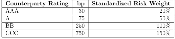
We calculate all valuation adjustments for 4 different counterparty ratings and spread combinations, AAA, A, BB and CCC. The spreads assumed in each case are given in table 2 alongside the risk-weight that is applied in the standardized CCR calculation. The counterparty recovery rate is assumed to be 40%.

Counterparty Rating bp Standardized Risk Weight

AAA 30 20%

A 75 50%

BB 250 100%

CCC 750 150%

Table 2: Counterparty spread data used in the examples.

The results of the example calculations are given in table 3. Setting aside the Market Risk component of the capital we see that KVA from CCR and CVA terms gives an adjustment of similar magnitude to the existing CVA, DVA and FCA terms, demonstrating that KVA is a significant contributor to the price of the derivative.

The market risk is assumed to be unhedged and so this KVA component is relatively large compared to the CCR and CVA terms. Under the standardized approach to market risk the capital requirement on a ten year transaction of this type is scaled according to a 60 bp move in rates. Practical applications would calculate the market risk capital requirement over all trades in a portfolio and then attribute these to trade level.

Comparing the Capital Allocation and Capital Insurances cases shows a re-duction in capital costs if capital is used to offset losses on counterparty default. This reduction becomes increasingly significant with increased probability of counterparty default.

6

Conclusions

We have presented a unified model for valuation adjustments that includes the impact of Capital and in so doing have introduced a new “XVA” term, KVA. The impact of capital upon the default of the counterparty has been explored giving two cases, Capital Allocation and Capital Insurance. We have described how KVA can be calculated in the case of the formula based approached to regulatory capital calculation and sketched how this may be calculated in the case of internal model approaches. Practical examples of KVA on an interest rate swap have demonstrated how significant capital costs are and that KVA is broadly similar in size to the other components of XVA. The assumption of Capital Insurance results in significant reductions in KVA for counterparties with a high probability of default.

References

BCBS-189 (2011). Basel III: A global regulatory framework for more resilient banks and banking systems. Basel Committee for Bank Supervision.

BCBS-219 (2012). Fundamental review of the trading book — consultative document.Basel Committee for Bank Supervision.

BCBS-254 (2013). The non-internal model method for capitalising counter-party credit risk exposures - consultative document.Basel Committee for Bank Supervision.

BCBS-261 (2013). Margin requirements for non-centrally cleared derivatives.

Basel Committee for Bank Supervision.

BCBS-265 (2013). Fundamental review of the trading book - second consul-tative document. Basel Committee for Bank Supervision.

BCBS-267 (2013). Second report on the regulatory consistency of risk-weighted assets in the trading book issued by the Basel Committee.Basel Committee for Bank Supervision.

Burgard, C. and M. Kjaer (2011). Partial differential equation representa-tions of derivatives with bilateral counterparty risk and funding costs.

The Journal of Credit Risk 7, 75–93.

Burgard, C. and M. Kjaer (2013). Funding Strategies, Funding Costs.

Risk 26(12).

Department of the Treasury (2013). 12 CFR Parts 208, 217, and 225. Regula-tory Capital Rules: RegulaRegula-tory Capital Rules: RegulaRegula-tory Capital, Imple-mentation of Basel III, Capital Adequacy, Transition Provisions, Prompt Corrective Action, Standardized Approach for Risk-weighted Assets, Mar-ket Discipline and Disclosure Requirements, Advanced Approaches Risk-Based Capital Rule, and Market Risk Capital Rule; Final Rule. Federal Register, Vol. 78(198), pp62017-62291. Department of the Treasury.

Dodd, C. and B. Frank (2010). Dodd-Frank Wall Street Reform and Con-sumer Protection Act. H.R. 4173, http://www.sec.gov/about/laws/ wallstreetreform-cpa.pdf.

EBA (2013). On prudent valuation under Article 105(14) of Regulation (EU) 575/2013. Technical report, European Banking Authority. EBA-CP-2013-28.

EU (2013a). Directive 2013/36/EU of the European Parliament and of the Council of 26 June 2013 on access to the activity of credit institutions and the prudential supervision of credit institutions and investment firms, amending Directive 2002/87/EC and repealing Directives 2006/48/EC and 2006/49/EC Text with EEA relevance.European Commission.

EU (2013b). Regulation (EU) No 575/2013 of the European Parliament and of the Council of 26 June 2013 on prudential requirements for credit insti-tutions and investment firms and amending Regulation (EU) No 648/2012 Text with EEA relevance.European Commission.

FCA (2014). Prudential Sourcebook for Banks, Building Societies and Investment Firms (BIPRU). Online; accessed 17 Feb 2014; http:// fshandbook.info/FS/html/handbook/BIPRU.

Kenyon, C. and A. Green (2013a). Pricing CDSs’ capital relief.Risk 26(10).

Kenyon, C. and A. Green (2013b). Regulatory-Compliant Derivatives Pricing is Not Risk-Neutral.SSRN.http://ssrn.com/abstract=2349103.

Kenyon, C. and R. Kenyon (2013). DVA for Assets.Risk 26(2).