Monash University, Wellington Road CLAYTON Vic 3800 AUSTRALIA
from overseas: Telephone:
(03) 9905 2398, (03) 9905 5112 61 3 9905 2398 or
61 3 9905 5112 Fax:
(03) 9905 2426 61 3 9905 2426
e-mail: [email protected]
Internet home page: http//www.monash.edu.au/policy/
Solution Software for CGE Modeling
by
M
ark
HORRIDGE and Ken PEARSON
Centre of Policy Studies, Monash University
General Paper No. G-214 March 2011
ISSN 1 031 9034 ISBN 978 1 921654 21 3
by Mark Horridge and Ken Pearson
March 2011
Abstract
We describe the progress of computable general equilibrium (CGE) modeling software since the 1980s and contrast the main systems used today: GAMS, MPSGE, and GEMPACK. The development of these general-purpose modeling systems has underpinned rapid growth in the use of CGE models and allowed models to be shared and their results replicated. We show how a very simple model may be implemented and solved in all 3 systems. We note that they produce the same numerical results but have different strengths. We conclude by considering some challenges for the future.
JEL classification: C63, C68, D58.
1. Introduction 1
2. Early days 1
3. General-purpose software 3
3.1 Allow input intelligible to modelers 3
3.2 Handle a wide range of models 3
3.3 Insulate modelers from the solution method 4
3.4 Windows programs to control simulations and examine data and results 4
3.5 Run on different computers 5
4. Levels and change solution methods 5
1.1 Levels strategy and GAMS 6
1.2 Change strategy and GEMPACK 7
5. General features of CGE Models 8
5.1 Main equation groups of a model 8
5.2 The data-base is consistent with initial truth of the model equations 9
5.3 General features of model code 10
6. Three representations of a simple model 11
6.1 The SIMPLE model in GEMPACK 13
6.2 An example simulation 16
6.3 The SIMPLE model in GAMS 18
6.4 The SIMPLE model in MPSGE 24
6.5 All three give the same results 27
6.6 Understanding the results 27
7. The curse of dimensionality 28
8. Checking and debugging models 30
9. Comparison of GAMS and GEMPACK 30
10. Conclusion 32
10.1 What are the computational challenges ? 32
10.2 Transferring models between the software platforms 33
11. References 34
Tables
Table 1 Database for example model 11
Table 2 TABLO Input file for example GEMPACK model 14
Table 3 GEMPACK Command file for sample simulation 17
Table 4 Simulation results, 10% Improvement in Service labor productivity 17
Table 5 GMS Input file for example GAMS model and simulation 19
Table 6 GMS Input file for example MPSGE model and simulation 25
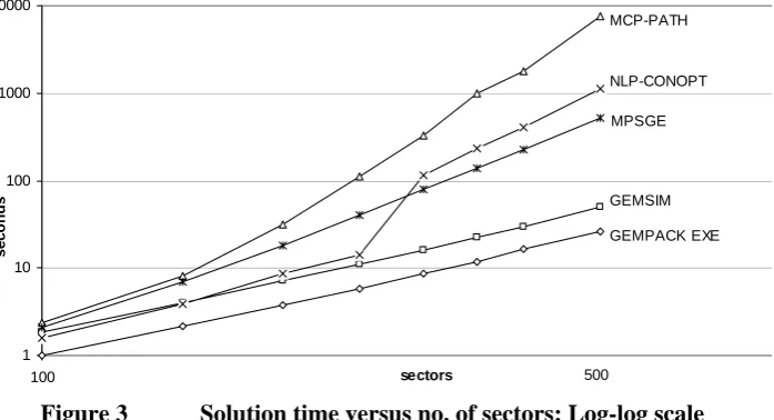
Table 7 Solution time (seconds) versus no. of sectors 29
Figures
Figure 1 Structure of input demands for industry i 12
Figure 2 Structure of non-export final demand 12
by Mark Horridge and Ken Pearson
1. Introduction
Since 1980 computable general equilibrium (CGE) modeling has evolved from a frontier technique practiced by a few specialists into a tool widely used by researchers in universities and other organizations. On the demand side, the growth has been driven by policy-makers' appetite for detailed analyses of issues which af-fect various sectors or interest groups in different ways. Increased supply of CGE analyses has been enabled by more powerful computers and better software. The latter, software, contribution is examined in this paper. CGE pioneers were required to develop their own model theory; construct their own database; devise a solution strategy and hire programmers to implement that strategy in a model-specific program. Thus new entrants to the field faced large upfront costs.
General equilibrium models require the numerical solution of large systems of equations, which in turn re-quires non-trivial computing power. Since the 1960s, a variety of mainframe computers offered this capacity. However, operating systems and computer language (eg, Fortran) implementations differed between manu-facturers. It was not easy to "port" a program from one computer to another. This hindered the spread of CGE modeling between sites, and made it hard for other modelers to replicate simulation results. Since CGE results rest upon a host of assumptions (not always documented completely or accurately), replicability—and the potential to recompute results with slightly different assumptions—underpins model credibility. Without these, the model remains an unconvincing "black box".
Standardization has been key to the spread of CGE modeling1. This includes:
1. Consensus about many (but not all) of the model's mechanisms; eg, the widespread use of nested CES to model substitution.
2. Standard data sources, such as the GTAP world dataset which provides data for several different CGE models; and accepted file formats to distribute such data.
3. Widespread use of x86 PCs, usually running Microsoft Windows. Such machines are now powerful enough to run nearly all CGE models, and offer a standard computer environment: the program devel-oped in Palo Alto will run and give the same results in Bonn.
4. The use of a few software packages (GEMPACK, GAMS and GAMS/MPSGE2) to code and run most CGE models.
5. Training in CGE methods and software at special courses, in graduate study programs, or on-the-job in some large organizations, leading to a pool of CGE operatives with transferable skills.
6. A modest job market for CGE modelers—so that project staff can be replaced. Earlier modeling projects often withered when staff moved on.
These advances have allowed models to be widely shared, and have lowered development costs for new models. Standard CGE modeling software has contributed directly, and indirectly has supported advances 5 and 6 above. We concentrate here on the most widely used software—GAMS and GEMPACK—used by 80% or more of CGE modelers.
2. Early days
By 1980 CGE was already established as a field, with models described by Shoven & Whalley (1972), Taylor & Black (1974), Hudson & Jorgenson (1974), Dixon et al (1977), and Adelman & Robinson (1978). These models were solved with special-purpose programs, usually written in Fortran. Modelers wrote the theory using algebraic notation and then had to hire a computer programmer who converted the theory of the model to Fortran programs. There were often errors and other problems since the modeler could not
1 However, enough hetorodoxy and dispute remain to seed further advances.
stand the Fortran and the programmer could not understand the model. Model changes were difficult and costly. And it was almost impossible for models to be transferred from the originator to other research groups for checking, validation or use. Indeed, often the originator was unable to reproduce results obtained as little as 6 months previously.
These were serious problems.
The solution recognized gradually in both USA and Australia was to develop general-purpose software
which eliminated the need to write model-specific programs in Fortran. Such software could:
•handle a wide range of models (that is what we mean by "general-purpose"),
•accept input from modelers directly in a form which is intelligible to modelers,
•allow modelers to make changes quickly,
•allow modelers to concentrate on the economics (not the computing),
•allow modelers to reliably reproduce results obtained earlier,
•be used on a range of different computers.
The first general-purpose software used for CGE modeling was GAMS (General Algebraic Modeling System). GAMS was developed starting in the mid-1970s by Alex Meeraus and Jan Bisschop working at the World Bank. Its focus was the solution of large-scale, non-linear optimization problems.3 GAMS was adapted to CGE modeling at the World Bank in the mid-1980s. The first GAMS-based CGE model was by Condon et al (1987). Although GAMS was designed initially to handle non-CGE problems, notably optimi-zation problems, we will only discuss the CGE capabilities of GAMS in this paper.
Coming out of Rutherford's PhD thesis (1987) was a second implementation of general-purpose software, MPSGE (Mathematical Programming System for General Equilibrium analysis). This operates as a subsystem within GAMS.
Meanwhile, in Australia, the ORANI model was being used widely for policy analysis. In the early 1980s ORANI was solved on the CSIRO mainframe computer. Modelers had to submit their jobs on cards and wait overnight for their simulation to run. As will be seen below (section 4.2), solving ORANI required the re-peated solution of large systems of linear equations. Pearson suggested that sparse solver techniques would speed up the solution of the model and delivered software to implement these techniques. Then, realising that model implementation and changes were very difficult (because the model was coded in model-specific Fortran), he undertook to develop general-purpose software GEMPACK (General Equilibrium Model PACKage) aimed especially at solving ORANI and related models.
The first version of GEMPACK was used for teaching in 1984, and shortly after that was adopted by Aus-tralian CGE modelers. The first GEMPACK manuals were published in 1986 (see Codsi and Pearson, 1986). Early journal descriptions of GEMPACK are Pearson (1988) and Codsi and Pearson (1988). Early versions of GEMPACK only produced Johansen (1-step) solutions which are not accurate, especially for large changes. The first version of GEMPACK which was able to produce accurate solutions of the underlying nonlinear model was Release 4.2.02 (April 1991). Hertel et al (1992) compared the North American levels methods with the Australian GEMPACK-based methods for implementing and solving GE models and showed that the differences were those of style rather than substance since the alternative model representations (linear or levels) and solution methods produce the same results. Early standard GEMPACK-based models producing accurate solutions were documented in Hertel et al (1997) and Horridge, Parmenter and Pearson (1993).
By the mid-1990s, nearly all policy-important CGE models were implemented and solved using one of GAMS, MPSGE or GEMPACK. For this reason we only discuss these 3 software suites below.
Of course it is still possible to implement and solve CGE models using other software, including spread-sheets, Mathematica, Matlab and special-purpose code. But if you want your model to be understood by other policy modelers, it pays to use software familiar to them.
GAMS, MPSGE and GEMPACK make it easy to transfer models around the world and to reproduce model results. Most models implemented with one of these could, at least in principle, be implemented with either of the other two and yield the same results.
3. General-purpose software
As mentioned above, a key motivation in designing and adopting general-purpose CGE software was to allow economists to construct and run models without being (or hiring) computer programmers or algorithm experts. So the software should make the normal tasks of specifying models, setting up and solving simulations, looking at results and writing reports as straightforward as possible. If modelers can do these things without too much effort, they are able to concentrate on the economics of their model and simulations. Thus they are able to do qualitatively better policy analysis.
We describe below some of the main features common to today's CGE modeling systems.
3.1 Allow input intelligible to modelers
Each of GAMS, MPSGE and GEMPACK requires that model equations be specified in a text file, using a special syntax.
For GAMS and GEMPACK the syntax resembles standard algebraic notation used in economic text books. For example, the Leontief equation for demands for commodities by industries:
Xij = AijZj i∈COM, j∈IND might be rendered for GAMS as:
E_X X(i,j) = A(i,j) * Z(j);
where subscripts i and j have been previously assigned to the sets COM and IND.
GEMPACK was originally developed for modelers used to working with the ORANI model, in which equations were written down in linearized form (relating percentage changes rather than the levels values of the variables involved). Following this tradition, for GEMPACK we would normally4 write down the percent-change (log-change) form:
E_x (all,i,COM)(all,j,IND) x(i,j) = a(i,j) + z(j);
where the lowercase symbols x, a, and z are understood to be percent changes from the initial values of X, A and Z.
Often it is clearer to explain the main features of CGE models in words, together with diagrams that show the structure of data and substitution (nesting). MPSGE builds on this way5 of explaining models, using a concise text summary of accounting constraints and nesting structure. It assumes that most substitution be-havior can be described using nested CES functions. The MPSGE representation of a model is typically rather compact.
All three systems make it fairly easy to specify (or change details of) a CGE model.
The use of the three different modeling languages is further illustrated in Section 6, which shows GAMS, MPSGE and GEMPACK representations of the same basic model.
3.2 Handle a wide range of models
While most CGE models bear a strong family resemblance, there are many differences between them. General-purpose software should be able to handle the range of CGE models used for policy analysis. Both GAMS and GEMPACK satisfy this requirement, since they allow nearly any equation to be represented. Indeed neither system contains any economics, or enforces any preconception of how a CGE model works. Either system could be used for non-CGE purposes: to compute, say, the stresses in a bridge design. The modeler is obliged to encode all economic theory used by his model into the text specification—making every assumption explicit. He is of course free to include equations which are wrong, perhaps because of typos.
By contrast MPSGE does enforce a framework or template for models—which is however flexible enough to represent nearly all of the equations used in most CGE models. Within this framework, a beginner has more chance of specifying even a fairly complex model correctly. To model behavioral specifications which
4 GEMPACK also accepts equations written in levels form. 5 GAMS/HERCULES [Drud
et al.,1986, 1989] took this approach even more strongly since the structure of the SAM drove model
lie outside the basic framework, MPSGE allows exceptions to be made—at some cost to the brevity and clarity of the model code.
All three systems can handle models which are large—either because there are many equation blocks and/or because the number of sectors or regions is large. In either case such a model may be computationally demanding.
All three systems can handle models with varying levels of aggregation. For example, GTAP supplies a world model dataset with 57 sectors and >100 regions—too big to solve quickly. Modelers must first reduce the size of the database by combining sectors and regions into groups, defined according to the needs of a particular simulation. The same model code can be used with any aggregation of the database—sets (ie, lists) of regions and sectors can be read from the database at runtime.
3.3 Insulate modelers from the solution method
A CGE model is a large system of simultaneous non-linear equations—to solve it presents a considerable computational challenge. Hence early CGE modelers were, perforce, amateur practitioners in the field of numerical algorithms. During the 1970s several approaches contended, including:
•Programming approaches, motivated by the wide success of the Simplex algorithm, and by the idea that a CGE model can be recast as a single-optimand optimization problem. While attractive for very simple models with no distortions, this approach becomes less practical where there are multiple optimizing agents facing a range of tax and other distortions.6
•Scarf (1967) and related algorithms which constructed a set of equilibrium prices. These were briefly favored but discarded as slow.
•Iterative methods such as Jacobi, which required (a) a model-specific assignment of variables to equations, and (for Gauss-Seidel) a suitable ordering of equations.
•Other methods, such as Newton-Raphson or conjugate gradient. Today practice has converged to a common paradigm:
•The system of equations is square: the number of equations equals the number of endogenous variables.
•The solver allows a flexible assignment of variables between exogenous and endogenous groups.
•The modeler is not required to understand the internals of the solving engine: it is a "black box" to him.
•The solving engine does not understand the economic intent of the modeler; eg, it does not know which variables are prices and which are quantities.
•Some or all of the model equations may be expressed as complementarities.
•An initial solution is provided which satisfies all (or nearly all) of the equations.
GEMPACK provides a single solution algorithm to satisfy these requirements. GAMS is designed to inter-face with a range of solvers, but most of these are optimizing7 packages. However the PATH solver (and its lighter-duty cousin, MILES) are direct equation solvers. Alternatively, optimizers such as MINOS or CONOPT could be used with a dummy optimand.
3.4 Windows programs to control simulations and examine data and results
Prior to the introduction of MsWindows, command-line programs were used to solve CGE models. The modeler needed to remember the right operating system commands, and the names and location of files used. To examine input data and simulation results, voluminous printouts were needed. The computing experience was laborious and annoying.
Both GAMS and GEMPACK now provide Windows programs which greatly facilitate these tasks. For example, the GAMS IDE allows the user to run and manage simulations without ever seeing the command line. It remembers the right file names, and offers a data viewer to directly view 2- or higher-dimensional matrices contained in binary files. GEMPACK offers a similar general-purpose IDE (WinGEM), which is supplemented by half a dozen more specialized programs—for viewing and editing code, data or results. There is a special IDE for running recursive dynamic programs.
6 Dixon (1975) proposed a method of constructing an artificial optimand, which corrected for distortions and multiple agents. Rutherford (1999) explores a similar idea.
These programs, particularly the data viewers, have greatly increased modelers' productivity. Models with many sectors, regions, or periods produce a volume of results which it would be impossible to inspect in print form.
Some of the GEMPACK IDE's have another useful feature: they can identify and zip up all of the original or source files needed to reproduce a simulation. Hence, modelers can archive all ingredients of their results, can retrieve and reproduce them fairly quickly and can send them to others (perhaps in different countries) who can do the same.
3.5 Run on different computers
While today most CGE modelers work on a Windows PC, in the 1980s GAMS and GEMPACK needed to be portable across a range of computers and operating systems. Even up to the mid 1990s, the limited capacity of Windows PCs meant that larger models were sometimes solved on mainframes or UNIX computers. For example, the Australian Industry Assistance Commission (IAC) was the custodian of the ORANI model in the 1980s. Policy modelers were able to run ORANI on one mainframe computer, using model-specific and operating-system-model-specific Fortran code8. Around 1989, the cost of using this computer became prohibitive. But the ORANI solution code would only run on it and rewriting it would have taken several months. The IAC approached Pearson to see if the fledgling GEMPACK could solve ORANI on the new (and relatively inexpensive) IBM-like mainframe NAS computer they had purchased. Because GEMPACK was written using ANSI standard Fortran instructions, it was possible to port GEMPACK to the NAS and solve ORANI there within two weeks.
Portability remains in 2011, at least for the core, command-line, GAMS and GEMPACK solution programs, which can be run under, eg, Linux or Mac environments. Unfortunately the almost-indispensable Windows IDE/viewer programs are not so portable. At the same time, the introduction of 64-bit Windows means that Windows users need suffer no performance penalty. Consequently non-Windows use is mostly confined to a small band of Linux or Mac enthusiasts—and most of these will still use Windows viewer programs (either on another computer, or within a Windows emulator running under their preferred OS). However, Windows' dominance is not quite complete. Where a CGE model is part of a larger software system—such as the 'Integrated Assessment' systems which link economic and physical models—it may be necessary to run the combined system under Linux9. Computer clusters, which usually run Linux, might occasionally10 be useful for, say, running Monte Carlo simulations. In each case, economists would require additional IT help to use the system.
Finally, portability remains an insurance policy against future changes in computing environments.
4. Levels and change solution methods
A CGE model may be represented as a system of N simultaneous non-linear equations:
F(Z) = 0
The variables Z may be divided into N endogenous variables Y, which are determined by the system, and the
remaining variables X (the exogenous ones). So we may write: F(Y, X) = 0
As explained below, in CGE practice we assume that we know an initial solution [Y0, X0]: F(Y0, X0) = 0
We wish to find another solution with different settings of some exogenous variables:
F(Y1, X1) = 0
8 The story here is in no sense a criticism of the original ORANI code written by John Sutton. On the contrary, to be able to solve ORANI with the tiny (by today's, or even late 1980s, standards) memory available on computers in the late 1970s was a veritable tour de force. Computers improved massively during the 1980s.
9 Essentially because some scientists and their programs will only run under Linux.
and to report percentage differences between Y1 and Y0.
Some or all equations may be defined via complementarities. Each complementarity equation Fi has an associated variable Zi which is bounded between U and L. Then just one of these three relations will hold:
F
i(
Z) = 0
and
L
i≤
Z
i≤
U
iF
i(
Z) > 0
and
Zi = LiF
i(
Z) < 0
and
Zi = UiComplementarities are a convenient way to represent the first-order or Kuhn-Tucker conditions which arise from optimization by agents. But they may arise in many other contexts (eg, quotas, or stepped tax schedules).
4.1 Levels strategy and GAMS
The levels strategy is to search through various Y values to find a solution. The process is iterative; for
example we might improve the current values via a Newton-Raphson step:
FY(Y, X1).dy = – F(Y, X1)
where FY is the Jacobian matrix or derivative of F w.r.t. Y, and dy is the suggested set of revisions to the current Y values. We can measure how close we are to a solution with a merit function, for example FTF (the
sum of squared errors of the equations). The process stops (ie, we have a solution) when the merit function becomes sufficiently tiny. Near to a solution, convergence is usually very rapid (eg, halving of error at each step).
By design GAMS does not prescribe a particular search strategy for Y: this task is left to the variety of
solvers which may be used with GAMS. Industrial-strength solvers like PATH use a range of strategies. Amongst these, variants of Newton-Raphson play an important part—it may serve as an example here. What GAMS does do is:
•provide the modeler with a convenient interface for specifying the functions F, setting up values for X0, Y0
and X1, and invoking a solver.
•provide to the solver, on request, fresh evaluations of the functions F and the gradients FY, using the latest estimates of Y.
Considering the Newton-Raphson step:
FY(Y, X1).dy = – F(Y, X1)
we see it requires evaluation (by GAMS) of F and FY, and solution (by the solver) of a large linear system. All three operations are costly; GAMS (and the solvers) work to reduce costs in many ways. For example, because most variables appear in only a few equations the Jacobian matrix FY is mostly zero: GAMS' sparse storage scheme processes only the non-zero elements.
Levels solution algorithms are not indifferent to units of measurement. Suppose we declare that equations are solved if FTF<10-6 . The criterion will be affected by the units we choose for Z (whether, say, thousands or millions of dollar). Consequently:
•GAMS modelers should scale their data appropriately
•We can imagine changes in exogenous variables that are too small to notice. That is, if we have an initial solution such that F(Y0, X0)TF(Y0, X0) <10-6, we could find small changes ε in exogenous variables such
that F(Y0, X0+ε)TF(Y0, X0+ε) was also <10-6. Hence we need to ensure that shocks rise above the
back-ground level of numerical noise—we cannot directly compute the dollar change in GDP that might occur if we added one dollar to national health spending. Instead we might simulate the effect of a million dollar increase—then divide simulated changes by one million.
GAMS reduces these problems by working with double precision arithmetic, which is accurate to 16 signifi-cant figures. However, compared to single precision arithmetic, double precision approximately doubles memory needs and execution time11.
4.2 Change strategy and GEMPACK
GEMPACK's solve strategy requires that we start from a solution, ie:
F(Y0, X0) = 0
For small changes dy and dx, in the neighborhood of a solution, we have the linear system FY(Y, X).dy + FX(Y, X).dx = 0
which we could solve to give:
dy = – [FY(Y, X)]-1FX(Y, X).dx
The above is a linear or first order approximation, accurate only for very small changes.12 However, we can reduce the error as much as we like by dividing the exogenous changes ΔX=X1–X0 into N equal parts and
re-peatedly imposing 1/Nth of the shock to the equation above. After each step, X and Y change, so that we
need to re-evaluate FY and FX. This is the Euler13 method of solving differential equations, with the following characteristics:
1. As the number of steps N increases, we get a more accurate answer.
2. Unlike the Newton-Raphson method, we never need to evaluate F. However, we still need, at every step,
to evaluate the derivative matrices FY and FX, and to solve a large linear system.
3. Compared to Newton-Raphson, Euler is more stable, but slower to reach accurate answers. We find usually that to halve the error we need to double the number of steps N.
The last point (3) seems to make Euler less attractive than Newton-Raphson, which often halves the error at every step. Besides, the comfort of (1) is diminished by (2): without evaluating F, how can we know how
accurate our solution is, or whether we need to increase N?
The second, accuracy, concern is addressed as follows: we can perform 3 Euler simulations with, say, 4, 8 and 16 steps; then compare results. Then we can use these 3 estimates of the true answer to calculate a new estimate by Richardson extrapolation. The extrapolated estimate is typically far more accurate than any of its components; it is equivalent, say, to a 1000-step Euler calculation. As well, the extrapolation generates error bounds for each results, so we can tell if our estimate is accurate enough (if not, more steps are needed). The first worry, that so many Euler steps may be slow, is addressed by:
•using industrial strength linear solution routines, prepared at Harwell Labs, UK (see Duff et al, 1989)
•recasting the linearized equation system using percent change variables. This turns out to eliminate a great deal of computation.
•using automatic algebraic substitution of high-dimension linearized equations to enormously reduce the size of the linear system.
4.2.1
Simple linearized equations enable substitution
In a typical GEMPACK model, most of the change variables are expressed as percentage changes (rather than ordinary changes). Thus, the levels GAMS equation:
x(c,s,u)=A_ARM(c,s,u)*xcomp(c,u)*[pcomp(c,u)/p(c,s)]**SIGMA(c);
which describes import-domestic substitution by user u for commodity c, becomes, in percent change form: x(c,s,u) = xcomp(c,u) ‐ SIGMA(c)*[p(c,s)‐pcomp(c,u)];
The percent change form is simpler, and uses cheaper arithmetic operations: powers are replaced by products, and products by sums. Moreover, GEMPACK code will contain commands like:
Backsolve x using E_x;
which instructs the system to drop the above equation, and simultaneously replace each occurrence of x in other equations by {xcomp(c,u) - SIGMA(c)*[p(c,s)-pcomp(c,u)]}. This can greatly reduce the number of
equations in the system, and is easy to do for linearized equations.
12 But accurate indeed for tiny changes: in this case, we can directly simulate a one dollar increase in health spending.
13 Press et al.(1992) think that the Euler method is useful for pedagogical purposes, but too crude for real-world use. By contrast, GEMPACK's experience with Euler has been positive; and the potential for users to understand how it works is a useful bonus. Many of the tricks used by GEMPACK to improve or build on Euler are described in Chapter 16 (ibid), "Integration of Ordinary
5. General features of CGE Models
Although exhibiting great variety, CGE models tend to share various characteristics. Below we describe a common core of features from which most models depart only in a few respects. Naturally the solution soft-ware has been adapted to cope efficiently with the most usual model features.
Like their progenitor, input-output modeling, CGE models focus on the production of commodities by industries – distinguishing from 10 to 1000 sectors. The commodities are demanded by industries and by final demanders (household, investment, government and export). Income arising from primary factor rents and from taxes and transfers is distributed to (and drives spending by) "institutions" such as households, cor-porations, government and foreigners.
5.1 Main equation groups of a model
Industry input demands are usually assumed to be proportional to output (constant-returns to scale is assumed) and sensitive to relative prices. These demand functions arise from the assumptions (a) that pro-duction (output) is a function of input quantities and (b) that producers choose the cheapest combination of inputs that will produce a given output.
The assumptions impose some (triad) restrictions on the form of input demands—but leave open a wide range of substitution possibilities. To tie these down, it is usual to impose additional, separability, assump-tions. For example, if an industry has multiple inputs and multiple outputs, we may stipulate an activity index Z such that:
F(inputs) = Z = G(outputs)
That is, a sector will choose the cost-minimizing mix of inputs to produce Z, and, given Z, will choose (subject to G) a revenue-maximizing output mix. The implication is that input mix is independent of output mix, or that large blocks of cross-price elasticities are zero, greatly simplifying computation and elasticity estimation. Very often the F function will also be separable via:
F(inputs) = H( I(primary factors), J(material inputs))
Similarly an industry's choice of how much, say, flour, to use, will be modeled independently of the choice whether to use domestic or imported flour. Household, government, and investment demands are modeled in a similar way.
Thus complicated demand systems are built up from a series of sub-aggregator functions, called nests. Usually the functional forms used are of the CES type, or are generalizations of CES. Diagrams of the nest-ing structure is often described by a diagram, like Figure 1 in Section 6.
The remaining core equations of the typical CGE model are fairly simple, consisting of:
• market-clearing equations which add up total demands for each good, and, for domestic goods, equate demand to domestic output.
• price equations which relate tax-inclusive user prices to output or CIF prices.
• income equations which add up total revenue accruing to each agent.
Usually there will in addition be equations defining common macro aggregates such as GDP or absorption; and model-specific equations defining, say, wage-indexation assumptions or rules for investment and capital accumulation.
5.1.1
Block equations: industry detail captured in matrices of numbers
5.1.2
Data: SAM plus elasticities
The typical CGE model database consists of:
• Matrices of transaction values, showing, for example, the value of coal used by the iron industry. Usually the database is presented as an input-output table or as a social accounting matrix. In either case, it covers the whole economy of a country (or even the whole world), and distinguishes a number of sectors, commodities, primary factors and perhaps regions or types of household.
• Elasticities: dimensionless parameters that capture behavioral response. These include the CES substi-tution parameters that underlie nested production and demand structures, and export demand or household expenditure elasticities.
The SAM structure, which arranges all flows into a single table according to the recipient (row) and payer (column) is a useful conceptual and pedagogical tool. In practice it can become inconvenient for large or detailed models since the SAM becomes too large or sparse to view easily. Also, the need to distinguish all flows through only 2 subscripts is constricting. For example, if we distinguish goods by sector and source and households by income and region, the natural way to record household demands is:
V(i,s,d,r) spending on good i from source s by income decile d in region r ie, to use 4 subscripts. In a 2-subscript SAM schema, this appears as
V(g,h) spending on good g by household type h
where subscript g runs over a compound set containing all combinations of good and source, and subscript h similarly combines all deciles and regions. Often therefore CGE flows data which could in principle be com-bined into an enormous, mostly-zero, SAM, are instead stored as a series of multidimensional matrices representing the non-zero blocks of a hypothetical SAM.
Usually these data are stored in a binary file of proprietary format14. While both GAMS and GEMPACK are able to read data in text or spreadsheet formats, binary storage is more compact and faster to process, especially for large models.
5.2 The data-base is consistent with initial truth of the model equations
Typically the flows database represents a single year and is assumed to be consistent with all (or nearly all) of the model equations. This point deserves elaboration.
Suppose that intermediate input demand by sector j for good i (Xij) is given by the Leontief function: Xij = AijZj
where Zj is output of sector j and Aij is a technological parameter. None of these variables appear in the model database, which only supplies:
Vj = PjZj the value of output of sector j, and Vij = PiXij the value of good i used by sector j
To obtain initial values for the variables we need to make assumptions—this is called calibration. For example, we might assume that both Pj and Pi were 1. Given the flow values, we could then deduce the quantities Xij and Zj, and thence calculate Aij. Clearly such a procedure guarantees (or assumes) that the demand equation is initially true.
The assumption that initial prices are 1 amounts to no more than an arbitrary choice of physical units for quantities like 'light industrial" output or demand for "other services" that have no natural unit of measure-ment. Because of this, it is meaningless to report simulated levels values of prices and quantities, except in relation to their initial values. So, universally, CGE model results are presented in terms of percentage changes from the initial levels values.
One might ask, would results for a given simulation be affected if we had assumed that Pj=2 and Pi=3 (instead of both 1). Clearly both initial and final levels results would be affected, but the percentage change results would be the same—otherwise we would reject the model or calibration process.
Like physical units, monetary units are irrelevant to percentage change results. We could halve all initial data flow values (converting from dollars to pounds) without altering the percentage change results from any simulation.
The database also stores various elasticities which affect behavior. By definition, these are unitless—so initial levels values are important. They are not 'free' in calibration. Consider the CES equation:
K/L = A.(PL/PK)σ
Assuming prices to be 1, and given initial flow values of capital and labor demand, we can deduce K and L and so deduce A. The value of σ must be supplied15.
It follows from this discussion that the whole useful content of a CGE model could be contained in a matrix function F:
[p , q ] = F(D, E, t, a)
where p and q represent finite16 percent changes in endogenous model variables; D represents various matrices of shares or ratios derived from the SAM or IO database; E is the set of elasticities; and t and a are percent changes in exogenous variables such as tax rates or technological coefficients17. Both the GEMPACK and the MPSGE ways to represent a CGE model draw on this insight.
The format of matrix function F above minimizes computation cost in the sense we only need to compute and store D and E (the initial database) and p, q, t and a (the results we need to report). That is, an average of 3 values per cell in the original IO table (p, q, D)18. A full levels-based approach is more expensive, since we need to store and compute the:
•original flows values V0, prices P0, quantities X0 and technological coefficients A0
•post-solution values of P and X, (these were initially set to P0 and X0)
•percentage changes p and q calculated as p=100(P/P0 - 1) and q=100(Q/Q0 - 1)
That is, an average of 8 values per cell in the original IO table. The load is more than doubled19, just to support the fictional construct of levels values.
5.3 General features of model code
For both of the two main CGE modeling systems, GAMS and GEMPACK, plain text files are used to specify the CGE model. In GAMS the same text file could also specify several individual simulations: GEMPACK requires that each simulation is specified by its own file, separate from that specifying the model.
Both GAMS and GEMPACK provide their own computer languages, to describe model and simulations. As in most computer languages, entities such as sets or variables must be described or 'declared' before they are used. This imposes an overall structure on model specification files:
•The first step is to define, either by direct enumeration or by reading from a file, the size and contents of various key sets—of sectors, regions, and so on.
•Next, data arrays are declared and their values are read from file.
•More data arrays are declared and given values which are derived from file data.
15 The alert reader will notice that, with initial price ratio 1, a shock to σ will have no effect; yet with non-uniform initial prices, a shock to σ (holding A fixed) would have an effect—contradicting the claim that assumed initial prices do not affect percent change results. The short retort might be that this is why mature CGE modelers never shock elasticities. A longer answer might explore the way in which different ways of writing the CES functions, which are generally agreed to be equivalent, in fact act differently if σ is considered to be a variable.
16 The percent changes are not infinitesimal and F is non-linear.
17 The conclusion depends only on the need for model results to be independent of arbitrary choice of units, and requires no
controversial neo-classical assumptions. For example, money illusion or increasing-returns-to-scale could be incorporated, if desired, via additional elasticities in the database.
•Next, in GAMS code, units of measurement are assigned (usually by setting prices), and numerous multi-plicative constants are computed. The logarithmic form of percent-change equations obviates the need for this step in GEMPACK
•Next the model equations are given, in levels or (for GEMPACK) in percent-change form.
•The closure, or choice of exogenous variables is specified.
•A GAMS model usually includes a no-shock simulation as a check; it should reproduce the benchmark data.
•An exogenous variable is changed, and a new solution computed.
•In GAMS, additional code is needed to derive percent-change results from old and new levels values.
6. Three representations of a simple model
We begin this section by showing the code for a fairly standard model which we call SIMPLE. We describe the model using data and nest diagrams, then give details of implementations20 in GEMPACK, GAMS and MPSGE.
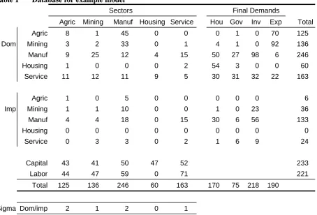
Table 1 below shows the model database. 5 competitive single-product industries (Agric ... Service) produce corresponding goods which are used by industries and final demanders. All non-export users also use imported goods, and industries also use Capital and Labor. There are no taxes in the model.
Table 1 Database for example model
Sectors Final Demands
Agric Mining Manuf Housing Service Hou Gov Inv Exp Total Agric 8 1 45 0 0 0 1 0 70 125 Dom Mining 3 2 33 0 1 4 1 0 92 136 Manuf 9 25 12 4 15 50 27 98 6 246 Housing 1 0 0 0 2 54 3 0 0 60 Service 11 12 11 9 5 30 31 32 22 163
Agric 1 0 5 0 0 0 0 0 6
Imp Mining 1 1 10 0 0 1 0 23 36 Manuf 4 4 18 0 15 30 6 56 133
Housing 0 0 0 0 0 0 0 0 0
Service 0 3 3 0 2 1 6 9 24
Capital 43 41 50 47 52 233
Labor 44 47 59 0 71 221
Total 125 136 246 60 163 170 75 218 190
Sigma Dom/imp 2 1 2 0 1
Demands are structured by a series of nests. For industries, the production/demand structure is shown in Figure 1 below. Each industry combines domestic and imported equivalents into commodity-composites via a CES aggregator. The elasticity of substitution varies by commodity and is shown in the last row of the table above. Import/domestic shares vary by good and by user. Industries demand commodity-composites in proportion to output. Similarly, each industry combines capital and labor using a CES with value 0.5 to produce a primary-factor-composite which is also demanded in proportion to industry output.
Output p(i,"dom") z(i) Labor demands pfac("labor",i) xfac("labor",i) Primary Factor pfac_f(i) Capital demands pfac("capital",i) xfac("capital",i) Imported Agric p(c,"imp") x(c,"imp",i) Domestic Agric p(c,"dom") x(c,"dom",i) Composite Agric pcomp(c,i) xcomp(c,i) Composite Service pcomp(c,i) xcomp(c,i) Imported Service p(c,"imp") x(c,"imp",i) Domestic Service p(c,"dom") x(c,"dom",i) Leontief CES
σ = 2
CES
σ = 1
CES σ = 0.5
up to
Figure 1 Structure of input demands for industry i
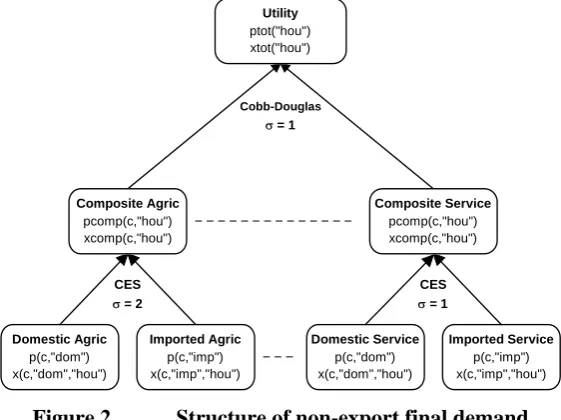
For the non-export final demanders (Hou, Gov and Inv) Figure 2 shows a similar structure except labor and capital are not used and the topmost nest is Cobb-Douglas rather than Leontief. Exports face foreign demand curves with a constant elasticity of –5.
Utility ptot("hou") xtot("hou") Imported Agric p(c,"imp") x(c,"imp","hou") Domestic Agric p(c,"dom") x(c,"dom","hou") Composite Agric pcomp(c,"hou") xcomp(c,"hou") Composite Service pcomp(c,"hou") xcomp(c,"hou") Imported Service p(c,"imp") x(c,"imp","hou") Domestic Service p(c,"dom") x(c,"dom","hou") Cobb-Douglas
σ = 1
CES
σ = 2
CES
σ = 1
Figure 2 Structure of non-export final demand
To close the model, we will assume that industry capital stocks are fixed, while Labor is mobile between sectors but fixed in aggregate. Aggregate nominal values of the Hou, Gov, and Inv demands are fixed pro-portions of nominal GDP. Other macro closures would be possible.
To be sure that our database is consistent with model equations (ie, that we can calibrate a solution—see Section 5.2), we need to check only two things:
(a) all the numbers are >= 0.
6.1 The SIMPLE model in GEMPACK
Table 2 shows how the model is specified using GEMPACK's TABLO language. The file starts by defining various sets. The list of sectors is read from a data file – so the same code could be used for a model with more or different sectors.
Next, the 3 data arrays (USE, FACTOR and SIGMA) are defined and their values read from file. The notation,
(all,f,FAC)(all,i,IND) FACTOR(f,i)
indicates that FACTOR is a matrix with 2 rows (Capital and Labor, the elements of set FAC) and 5 columns (the 5 sectors which form set IND).
Then, several other coefficients are defined which are all simple addups of USE and FACTOR. The Assertion statement is a safety check – the solver will terminate with an error if DIFF is not tiny.
As for most GEMPACK models, this simple model is specified in percent change form21. The model variables are listed next. By default, these are defined as percentage changes from the initial solution, except for the first, delB, which is an ordinary change.
As explained in Section 5.2, the percent change formulation allows us to express the model, and to compute percent changes in prices and quantities, without ever specifying initial values for prices and quantities (we only need initial flows). This enables brevity in model specification, and reduced computation time.
The equations which follow are all linear in percentage change variables, with coefficients that are data-base flows, addups of these flows, or elasticities. The first equation block:
E_pcomp # Price: dom/imp composites # (all,c,COM)(all,u,LOCUSR)
ID01[USE_S(c,u)]*pcomp(c,u)=sum{s,SRC,USE(c,s,u)*p(c,s)};
is a group of equations that define, for each good and local user, the first-order change in the CES price index of the composite good which combines domestic and imported versions. It states that pcomp(c,u) is a cost-share-weighted average of the percent changes in domestic and imported prices (Roy's Identity). The built-in function ID01 takes care of the case when use of the composite, USE_S(c,u), is zero: ID01(x)=x for all non-zero x, while ID01[0]=1. So in the degenerate case we have pcomp(c,u)=0. The name of the equation block, E_pcomp, is chosen to suggest that these equations can determine values of the variable pcomp. The next equation block:
E_x # Quant: final dom/imp composites# (all,c,COM)(all,s,SRC)(all,l,LOCUSR)
x(c,s,l) = xcomp(c,l) ‐ SIGMA(c)*[p(c,s)‐pcomp(c,l)];
specifies pairs (for s="dom" or "imp") of demand equations for each good and non-export user. We could subtract the imported from the domestic equation to demonstrate the CES property:
(all,c,COM)(all,l,LOCUSR)
x(c,"dom",l) ‐ x(c,"imp",l) = SIGMA(c)*[p(c,"imp")‐p(c,"dom")];
Many of the remaining equations follow similar patterns, or are simple addups of nominal values. As a check on the model's accounting relations, we have included two variables and equations for nominal GDP: we expect, from Walras' Law, that both variables will end up with the same value.
The equation for real GDP:
E_xgdp # Real GDP from income side #
VGDP*xgdp = sum{i,IND, sum{f,FAC, FACTOR(f,i)*[xfac(f,i)‐afac(f,i)]}};
is a Divisia index, not translated from any levels equation.
Table 2 TABLO Input file for example GEMPACK model
File INFILE # base data file #;
Set
COM # Commodities # read elements from file INFILE header "SEC";
IND # Industries # read elements from file INFILE header "SEC";
FIN # Final users # (Hou,Gov,Inv,Exp);
LOCFIN # Local final users # (Hou,Gov,Inv);
USR # All users # = IND + FIN;
LOCUSR # Local users # = IND + LOCFIN;
SRC (dom,imp);
FAC (Capital,Labor);
SEC = COM intersect IND;
Subset LOCUSR is subset of USR;
Coefficient ! data on file !
(all,c,COM)(all,s,SRC)(all,u,USR) USE(c,s,u) # Value of inputs #; (all,f,FAC)(all,i,IND) FACTOR(f,i) # Primary factor costs #; (parameter)(all,c,COM) SIGMA(c) # CES dom‐imp elasticity #;
Read
USE from file INFILE header "USE";
FACTOR from file INFILE header "FACT";
SIGMA from file INFILE header "SIG";
Coefficient ! calculated !
(all,c,COM)(all,u,USR) USE_S(c,u) # Value of import composites #; (all,i,IND) VALADD(i) # Factor costs #;
(all,u,USR) COSTS(u) # Costs #; (all,c,COM)(all,s,SRC) SALES(c,s) # Sales #; (all,q,SEC) DIFF(q) # Costs‐Sales #;
VGDP # GDP #;
Formula
(all,c,COM)(all,u,USR) USE_S(c,u) = sum{s,SRC, USE(c,s,u)}; (all,i,IND) VALADD(i) = sum{f,FAC,FACTOR(f,i)}; (all,u,USR) COSTS(u) = sum{c,COM, USE_S(c,u)}; (all,i,IND) COSTS(i) = COSTS(i) + VALADD(i); (all,c,COM)(all,s,SRC) SALES(c,s) = sum{u,USR, USE(c,s,u)}; (all,q,SEC) DIFF(q) = COSTS(q) ‐ SALES(q,"dom");
VGDP = sum{i,IND,VALADD(i)};
Assertion # Check data balance # (all,q,SEC) ABS[DIFF(q)]<0.001;
Variable
(change) delB # (Nominal balance of trade)/{nominal GDP} #;
xgdp # Real GDP #;
wgdpinc # Nominal GDP from income side #;
wgdpexp # Nominal GDP from expenditure side #;
phi # Exchange rate (local$/foreign$) #;
(all,c,COM) xexp(c) # Export quantities #;
(all,c,COM) fqexp(c) # Right shift in export demand curve #;
(all,i,IND) z(i) # Industry outputs #;
(all,c,COM) pfimp(c) # Imp goods prices, foreign $ #;
(all,l,LOCFIN) wtot(l) # Nominal expenditure by local final users #;
(all,l,LOCFIN) xtot(l) # Real expenditure by local final users #;
(all,l,LOCFIN) ptot(l) # Price indices for local final users #;
(all,f,FAC) xfac_i(f) # Total value‐weighted factor use #;
(all,f,FAC) ffac_i(f) # Factor wage shift #; (all,c,COM)(all,s,SRC) p(c,s) # Factor prices #;
(all,c,COM)(all,s,SRC) xdem(c,s) # Total demand for goods #; (all,f,FAC)(all,i,IND) pfac(f,i) # Factor prices #;
(all,i,IND) pfac_f(i) # Factor composite prices #; (all,f,FAC)(all,i,IND) xfac(f,i) # Factor use #;
(all,f,FAC)(all,i,IND) afac(f,i) # Factor‐using technical change #; (all,f,FAC)(all,i,IND) ffac(f,i) # Factor wage shift #;
Equation
! Dom/imp CES BLOCK !
E_pcomp # Price: dom/imp composites # (all,c,COM)(all,u,LOCUSR)
ID01[USE_S(c,u)]*pcomp(c,u)=sum{s,SRC,USE(c,s,u)*p(c,s)};
E_x # Quant: final dom/imp composites# (all,c,COM)(all,s,SRC)(all,l,LOCUSR)
x(c,s,l) = xcomp(c,l) ‐ SIGMA(c)*[p(c,s)‐pcomp(c,l)]; ! Industry demands !
E_pA # Industry cost indices # (all,i,SEC)
ID01[COSTS(i)]*p(i,"dom")=sum{c,COM,USE_S(c,i)*pcomp(c,i)}+VALADD(i)*pfac_f(i); E_pfac_f # Factor composite prices # (all,i,IND)
ID01[VALADD(i)]*pfac_f(i) = sum{f,FAC, FACTOR(f,i)*[pfac(f,i)+afac(f,i)]}; E_xfac # Factor demands # (all,f,FAC)(all,i,IND)
xfac(f,i) = z(i) + afac(f,i) ‐ 0.5*[pfac(f,i)+afac(f,i)‐pfac_f(i)]; E_xcompA # Local final demands (Cobb‐Douglas) # (all,c,COM)(all,i,IND)
xcomp(c,i) = z(i); ! Final demanders !
E_xcompB # Local final demands (Cobb‐Douglas) # (all,c,COM)(all,l,LOCFIN)
xcomp(c,l) + pcomp(c,l) = wtot(l);
E_wtot # Absorption # (all,l,LOCFIN) wtot(l) = wgdpinc; E_ptot # Price indices for local final users # (all,l,LOCFIN)
ID01[COSTS(l)]*ptot(l) = sum{c,COM, USE_S(c,l)*pcomp(c,l)}; E_xtot # Real expenditure by local final users # (all,l,LOCFIN)
xtot(l) + ptot(l) = wtot(l);
E_xexp # Export demands # (all,c,COM)
xexp(c) = fqexp(c) ‐5.0*[p(c,"dom")‐phi]; ! Total demands and market clearing !
E_ffac_i # Total (value‐weighted) factor use # (all,f,FAC)
sum{i,IND,FACTOR(f,i)*[xfac_i(f) ‐ xfac(f,i)]} = 0;
E_xdem # Total demand for goods # (all,c,COM)(all,s,SRC)
ID01[SALES(c,s)]*xdem(c,s) =
sum{l,LOCUSR,USE(c,s,l)*x(c,s,l)} + USE(c,s,"exp")*xexp(c); E_z # Market clearing # (all,i,SEC) z(i) = xdem(i,"dom"); ! Miscellaneous !
E_pB # Import prices # (all,i,SEC) p(i,"imp") = pfimp(i) + phi; E_pfac # Factor mobility/remuneration # (all,f,FAC)(all,i,IND)
pfac(f,i) = ptot("hou") + ffac(f,i) + ffac_i(f); E_wgdpinc # Nominal GDP from income side #
VGDP*wgdpinc = sum{i,IND, sum{f,FAC, FACTOR(f,i)*[pfac(f,i)+xfac(f,i)]}}; E_xgdp # Real GDP from income side #
VGDP*xgdp = sum{i,IND, sum{f,FAC, FACTOR(f,i)*[xfac(f,i)‐afac(f,i)]}}; E_wgdpexp # Nominal GDP from expenditure side #
VGDP*wgdpexp= sum{c,COM, sum{l,LOCFIN, USE_S(c,l)*wtot(l)}
+ USE(c,"dom","exp")*[p(c,"dom")+xexp(c)]
‐ SALES(c,"imp")*[p(c,"imp")+xdem(c,"imp")]}; E_delB # (balance of trade)/GDP #
100*VGDP*delB = sum{c,COM,USE(c,"dom","exp")*[p(c,"dom")+xexp(c)‐wgdpinc]}
‐ sum{c,COM,SALES(c,"imp")*[p(c,"imp")+xdem(c,"imp")‐wgdpinc]};
Update
(all,i,IND)(all,f,FAC) FACTOR(f,i)=pfac(f,i)*xfac(f,i);
(all,c,COM)(all,s,SRC)(all,l,LOCUSR) USE(c,s,l) = p(c,s)*x(c,s,l); (all,c,COM) USE(c,"dom","exp") = p(c,"dom")*xexp(c);
The rule for primary factor wages:
E_pfac # Factor mobility/remuneration # (all,i,IND)(all,f,FAC)
pfac(f,i) = ptot("hou") + ffac(f,i) + ffac_i(f);
is of a distinctively GEMPACK (or maybe Dixonian) form. At runtime the "f" variables (aka: shifters) will be set exogenous or endogenous to enforce different factor market closures. For example, if for capital we set ffac_i("Capital) exogenous and allowed the ffac(i,"Capital"), which appear nowhere else, to float endoge-nously, the equation would be otiose, merely determining changes in ffac. We could fix industry capital stocks, xfac(i,"Capital"), to determine the capital rents. For a slack Labor market we could hold both ffac("Labor",i) and ffac_i("Labor") fixed, so indexing wages to the CPI. Or we could fix both total Labor demand, xfac_i("Labor"), and the ffac("Labor",i) whilst allowing ffac_i("Labor") to float endogenously. The effect would be that industry wages would move together, to equate demand and supply for sectorally mobile Labor.
At the end of SIMPLE.TAB are Update instructions which tell GEMPACK how values on the data file are related to model variables. For example, the statement
Update (all,i,IND)(all,f,FAC) FACTOR(f,i)=pfac(f,i)*xfac(f,i);
indicates that the coefficient FACTOR is a product (in the levels) of prices PFAC and quantities XFAC. GEMPACK uses this information to update data flows after each step in the calculation. FACTOR is updated to become:
FACTOR(f,i)*[1+0.01*pfac(f,i)+0.01*xfac(f,i)] Finally, come backsolve statements such as:
Backsolve x using E_x;
This tells GEMPACK to perform algebraic substitution on the linear system, everywhere replacing x(c,s,u) by {xcomp(c,u) - SIGMA(c)*[p(c,s)-pcomp(c,u)]}. This enormously reduces the size of the equation sys-tem. The values of x are recovered and are available on the solution file. However, no element of x can be exogenous.
6.2 An example simulation
In GEMPACK, each simulation is specified using a separate file, suffixed ".CMF". Such a file is shown in Table 3 below. It starts by identifying the model, SIMPLE, described in the file SIMPLE.TAB (listed in Table 2). The name of the input file (simdata.har) is given. A file of identical format will be produced con-taining post-simulation (updated) values of all the data – this will be named after the CMF file.
On each line, any text following an exclamation mark is treated as a comment.
The next lines cause 3 Gragg simulations to be run, with 4, 6 and 8 steps. The final answers are produced by extrapolating from results of these 3 simulations.
Next comes the list of exogenous variables, or closure. GEMPACK users customarily begin from a well-known or standard closure; then, using "swap" statements, define differences from that well-known closure. In this case the reference closure is produced automatically by the software – it consists of all those variables which do not have an equation named after them. In this reference closure both labor and capital are mobile between sectors and fixed in aggregate – however we wish to fix industry capital stocks.
The statement:
swap xfac("capital",IND) = ffac("capital",IND);
causes the capital parts of the xfac variable (currently endogenous) to be set exogenous, while the capital parts of the ffac variable (currently exogenous) will become exogenous. This mechanism ensures that the number of endogenous variables (which must equal the number of equations) does not change. Having fixed the parts, we must endogenize the whole – this is done by a second swap statement.
Table 3 GEMPACK Command file for sample simulation
auxiliary files = simple;
log file = yes;
File INFILE = simdata.har; !
Updated File INFILE = <cmf>.UPD; ! will be named after CMF
method = GRAGG ;! Solution method
steps = 4 6 8;
! Automatic closure generated by TABmate Tools...Closure command ! Variable Size
Exogenous afac ; ! FAC*IND Factor‐using technical change
Exogenous ffac ; ! FAC*IND Factor wage shift
Exogenous fqexp ; ! COM Right shift in export demand curve
Exogenous pfimp ; ! COM Imp goods prices, foreign $
Exogenous phi ; ! 1 Exchange rate (local$/foreign$) [Numeraire]
Exogenous xfac_i ; ! FAC Total value‐weighted factor use
Rest endogenous; ! end of TABmate automatic closure ! new exogenous old exogenous
swap xfac("capital",IND) = ffac("capital",IND); ! fix industry capital stocks
swap ffac_i("capital") = xfac_i("capital"); ! unfix total capital stock
Verbal Description = Improvement in Service labor productivity;
shock afac("Labor","Service") = ‐10;
Results from the simulation are shown (as percent changes from base) in Table 4. First note that with aggre-gate nominal household, government and investment demands following nominal GDP, the residual balance of trade must also be a constant fraction of GDP. Service becomes cheaper, and that industry expands. Labor is released to other sectors, wages fall, and capital increases its share of national income (recall, the labor/capital CES is 0.5). Output increases in most sectors, especially Manuf and Service, while Agric and Mining, which are more export oriented, expand less. Housing output cannot rise because its capital stock is fixed and it uses no labor.
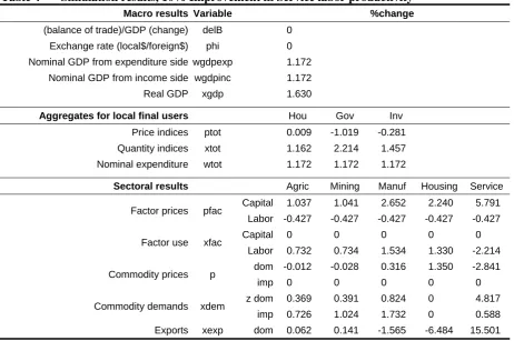
Table 4 Simulation results, 10% Improvement in Service labor productivity
Macro results Variable %change
(balance of trade)/GDP (change) delB 0
Exchange rate (local$/foreign$) phi 0
Nominal GDP from expenditure side wgdpexp 1.172
Nominal GDP from income side wgdpinc 1.172
Real GDP xgdp 1.630
Aggregates for local final users Hou Gov Inv
Price indices ptot 0.009 -1.019 -0.281
Quantity indices xtot 1.162 2.214 1.457
Nominal expenditure wtot 1.172 1.172 1.172
Sectoral results Agric Mining Manuf Housing Service
Capital 1.037 1.041 2.652 2.240 5.791 Factor prices pfac
Labor -0.427 -0.427 -0.427 -0.427 -0.427
Capital 0 0 0 0 0
Factor use xfac
Labor 0.732 0.734 1.534 1.330 -2.214
dom -0.012 -0.028 0.316 1.350 -2.841 Commodity prices p
imp 0 0 0 0 0
z dom 0.369 0.391 0.824 0 4.817 Commodity demands xdem
imp 0.726 1.024 1.732 0 0.588
Exports xexp dom 0.062 0.141 -1.565 -6.484 15.501
6.3 The SIMPLE model in GAMS
Table 5 below shows how the SIMPLE model may be implemented22 in GAMS. In this case a single GMS text file replaces the TAB and CMF file used by GEMPACK. As far as possible the same notation has been used as in the GEMPACK implementation. The chief difference is that although results are again reported as percentage changes, the model is specified in the levels. This means that for all quantities and prices, separate symbols must be defined to represent initial values, final values and percentage changes. In addition, the levels equations require a number of multiplicative constants (which drop out in percentage change form). The need to declare and assign values to all these parameters and variables takes a bit more space than needed in GEMPACK.
Section 1 of the GMS file reads in sets and data from the GDX file, and defines some additional sets. Then, zeroes in the factor payments data are replaced by tiny numbers, while the degenerate case where a CES = 1 is avoided. This simplifies subsequent code, although other approaches are possible. Next some useful add-ups of the input data are defined, and we check that industry costs equal domestic sales.
Section 2 declares initial values of all variables, and assigns values to these variables which are consistent with the base data. By convention, prices are set to 1 – then volumes are equal to initial flow values. Similarly Section 3 deduces technology and distribution parameters in production functions that are consistent with known prices and quantities.
Section 4 declares the model variables and equations. The variables are set equal to their initial values. A dummy variable, OBJ, serves as a maximand in case an optimizing solver is used (even though the system is fully constrained).
Section 5 begins by defining a standard set of exogenous variables (both factors mobile and fixed in aggre-gate) and performs a trial simulation without any shock. The aim is to check that the initial values do indeed constitute a solution. Next, the closure is altered so that industry capital stocks are fixed. A shock is imposed (10% cut in labor needed by services) and the model solved again.
Section 6 uses new and original values to compute a few percent-change results for reporting. The percent change in real GDP is computed as a Fisher (ideal) GDP quantity index—giving the same numerical result as the corresponding Divisia index in the GEMPACK model. Results are stored in a GDX file.
While the GEMPACK modeler automatically receives percent-change results for all variables, the GAMS modeler has to prepare formulae for each percent change. The path of least resistance is to compute percent-change results for only a few, summary, variables. In that case, detailed results, which could contain points of interest or even anomalies, may never be viewed.
Table 5 GMS Input file for example GAMS model and simulation
$Title Simple Model $OFFSYMLIST
$OFFSYMXREF $EOLCOM !
* Convention: variables (and initial values of variables) are in lowercase, * other parameters are in upper case
*======================== (1) Set Declaration ============================ * Declare and read Sets and Parameters stored in GDX
Set ! on data file
USR Users
FAC Factors
LOCUSR(USR) Local users
COM(LOCUSR) Commodities
IND(COM) Industries
LOCFIN(LOCUSR) Local final users
SEC(IND) Sectors
SRC Sources / dom, imp / ;
Parameter ! on data file
USE(COM,SRC,USR) Value of inputs
FACTOR(FAC,IND) Primary factor costs
SIGMA(COM) CES dom‐imp elasticity ;
$GDXIN input.gdx
$LOADdc USR, FAC, LOCUSR, COM, IND, LOCFIN, SEC, FACTOR, USE, SIGMA
Set ! Additional Sets
FIN(USR) Final users / Hou, Gov, Inv, Exp /
EXP(USR) Exports / Exp / ;
Alias (IND,i),(COM,c),(SRC,s),(USR,u),(FAC,f),(f,ff),(LOCFIN,lf),(LOCUSR,lu),(FIN,fu);
FACTOR(f,i)$(FACTOR(f,i)eq 0) = 1E‐9; ! alter data to avoid problems
SIGMA(c) $(SIGMA(c)eq 1) = 1.0001; !NOTE: CES sigma must not equal 1
Parameter ! addups of base data
VALADD0(i) Factor costs
COSTS0(i) Costs
SALES0(c,s) Sales
DIFF(i) Costs ‐ sales ;
VALADD0(i) = SUM[f,FACTOR(f,i)];
COSTS0(i) = VALADD0(i) + SUM((c,s), USE(c,s,i));
SALES0(c,s) = SUM(u, USE(c,s,u));
DIFF(i) = SALES0(i,"dom")‐ COSTS0(i);
DISPLAY VALADD0, COSTS0, SALES0, DIFF, FACTOR;
ABORT$(ABS{SUM[i, DIFF(i)]} GT 0.01)"!!!DATA BALANCE PROBLEM!!!";
*======================= (2) Parameter declarations ====================== Parameter ! initial values of variables (and variables) are in lower case
ffac0(f,i) Factor wage shift
pfac0(f,i) Factor prices
pfac_f0(i) Factor composite prices
xfac0(f,i) Factor use
xfac_i0(f) Total value‐weighted factor use
ffac_i0(f) Factor wage shift
xfac_f0(i) Total factor use by industry
z0(i) Industry outputs
x0(c,s,lu) Value of inputs
wtot0(lf) Nominal expenditure by local final users
xtot0(lf) Real expenditure by local final users
xdem0(c,s) Total demand for goods
xcomp0(c,lu) Quant: final dom‐imp composites
ptot0(lf) Price indices for local final users
p0(c,s) Goods prices
pcomp0(c,lu) Price: Intermediate dom‐imp composites for local users
wgdpinc0 Nominal GDP from income side
wgdpexp0 Nominal GDP from expenditure side
delB0 Trade balance
phi0 Exchange rate