Efficient Batch Zero-Knowledge Arguments for
Low Degree Polynomials
?Jonathan Bootle and Jens Groth
University College London, UK
Abstract. Bootle et al. (EUROCRYPT 2016) construct an extremely efficient zero-knowledge argument for arithmetic circuit satisfiability in the discrete logarithm setting. However, the argument does not treat relations involving commitments, and furthermore, for simple polynomial relations, the complex machinery employed is unnecessary.
In this work, we give a framework for expressing simple relations between commitments and field elements, and present a zero-knowledge argument which, by contrast with Bootle et al., is constant-round and uses fewer group operations, in the case where the polynomials in the relation have low degree. Our method also directly yields a batch protocol, which al-lows many copies of the same relation to be proved and verified in a single argument more efficiently with only a square-root communication overhead in the number of copies.
We instantiate our protocol with concrete polynomial relations to con-struct zero-knowledge arguments for membership proofs, polynomial eval-uation proofs, and range proofs. Our work can be seen as a unified ex-planation of the underlying ideas of these protocols. In the instantiations of membership proofs and polynomial evaluation proofs, we also achieve better efficiency than the state of the art.
Keywords: Sigma-protocol, zero-knowledge argument, batch-verification, discrete logarithm assumption.
1
Introduction
Zero-knowledge proofs and arguments allow a prover to convince a verifier that a particular statement is true, without revealing anything beyond that fact. More formally, the statement is an elementufrom an NP-languageL, and the prover convinces the verifier that there exists a witnesswto the fact thatu∈ L. They are useful both in theory and in practice, as they can be used to construct signature schemes, encryption schemes, anonymous credentials, and multi-party computation schemes with strong security guarantees.
Zero-knowledge arguments are computationally sound, meaning that cheat-ing the verifier to accept when u /∈ L reduces to breaking a computational
intractability assumption. In this paper, we focus on the discrete logarithm as-sumption. There are many examples of zero-knowledge arguments based on the discrete logarithm assumption, for both general, NP-complete languages such as arithmetic circuit satisfiability [7], and for simpler languages such as range and membership arguments, shuffle arguments, and discrete logarithm relations.
While very efficient, arguments for general statements often make use of generic reductions and complex machinery, and fail to be as efficient as arguments specialised for a particular language.
1.1 Contributions
In this paper, we aim to bridge the gap between general and simple languages. We do this in three ways.
Framework for Low Degree Relations. We provide a framework to describe the types of languages commonly encountered. Protocols such as the 1-out-of-N
membership argument of [28], and the polynomial evaluation argument of [2] prove membership in languages where the witnesses are zeroes of low-degree polynomial relations. In other words, the statement is an arithmetic circuit of low degree, and part of the witness is a satisfying assignment for the circuit. We give a general relation which allows us to recover specific protocols by instantiating with concrete polynomial relations. By separating the task of developing more efficient ways to perform the zero knowledge proof, and the task of designing better relations to describe a given language, we can explain the logic behind past optimisations of membership proofs in [28,6], and produce new optimisations for membership proofs and polynomial evaluation proofs.
Common Construction Techniques. We unify the approaches used in [28,2,6] to construct zero-knowledge proofs for membership and polynomial evaluation, which can all be viewed as employing the same construction method. The con-structions of zero-knowledge arguments for low degree polynomial relations in these works proceed by masking an input variableuasfu=ux+ub, using a ran-dom challengexand a random blinderub. During the proof, the polynomial or circuit from the statement is computed withfuin place ofu, so that the original relation appears in the leading x coefficient. The communication and compu-tational complexity of the resulting arguments is determined by the degree of the polynomial relation and the number of inputs. By contrast, the complexity of general arithmetic circuit protocols is determined by the number of gates. In the case of [7], the authors embed a polynomial evaluation argument for a poly-nomial of degreeN into a low degree polynomial with logN inputs and degree logN, obtaining a protocol withO(logN) communication using 3 moves, and requiring O(logN) exponentiations in a suitably chosen cryptographic group. On the other hand, a polynomial of degreeN requiresN multiplication gates to evaluate in general, so the best arithmetic circuit protocol [7] can only achieve
higher than that of computing finite-field multiplications in the discrete log-arithm setting, computing O(logN) group exponentiations rather than O(N) leads to a significant performance advantage when considering implementation on constrained devices.
Bayer [1] gives two efficient batch proofs for multiplication and polynomial evaluation, which achieve a square-root communication overhead in the number of proofs to be batched. The key to achieving square-root overhead in [1] is to use Lagrange interpolation to embed many instances of the same relation into a single field element. This technique can be applied more generally to produce efficient batch proofs for the low-degree relations described above. Furthermore, by combining this with the polynomial commitment subprotocol in section 3, we improve the communication cost of the batched proof from√tcto √tc, where
c is the communication cost of the original non-batched proof, and t is a large number representing the number of proofs to be batched together.
Efficient Protocols for Applications. We exhibit a general protocol in our frame-work, and give an efficient batch protocol for proving and verifyingtinstances of the same relation simultaneously. We then show how to recover protocols of pre-vious works with some optimisation. More specifically, we give new 1-out-of-N
membership arguments and polynomial evaluation arguments. Our new instan-tiations simultaneously decrease communication costs and reduce prover and verifier computation, while retaining the conceptual clarity and simple 3-move structure of the originals. As an example, we obtain the most communication efficientΣ-protocols for membership or non-membership of a committed value in a public list, in the discrete logarithm setting. We also include an argument for range proofs, which captures the folklore method for performing range proofs and demonstrates the expressivity of our general relation. Our arguments all possess the following desirable properties:
– Perfect completeness and perfect special honest verifier zero-knowledge. – Computational soundness based on the discrete logarithm assumption. – Simple 3-move public coin structure.
– Common reference strings are formed from random group elements. They require no special structure.
– Prover and verifier both have efficient computation.
The discrete logarithm assumption is well-known, well-examined, and widely used in cryptography. Our protocols rely on the discrete logarithm assumption in groups with prime order p. The assumption is believed to hold in suitable subgroups of elliptic-curve groups. The best algorithms for finding discrete loga-rithms in such elliptic curve groups are still generic algologa-rithms with complexity
Ω(√p). For these groups we therefore enjoy lower parameter sizes than protocols based on RSA groups that are subject to sub-exponential attacks.
known attacks. This makes protocols communicating large numbers of group el-ements highly impractical in this setting. As an improvement on previous works, in the case where t = 1 and we have a single relation, our protocols can be tuned so that they only require a constant number of group elements, resulting in much better efficiency when instantiated in finite fields of prime order, since the polylogλ3 λ communication cost can then appear as a constant additive factor rather than a multiplicative one.
As a building block in our arguments, we also present an adaptation of the polynomial commitment sub-protocol appearing in [7], which allows the prover to commit to a polynomial so that the verifier can learn an evaluation of the polynomial in a secure manner.
1.2 Efficiency
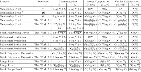
Figure 1 compares the efficiency of our protocol with other works. One notable place where we improve communication efficiency over previous proofs is in our membership and polynomial evaluation proofs, which use a constant number of group elements, but have better communication efficiency regardless of whether the proofs are instantiated in elliptic curve groups or multiplicative subgroups of finite fields. Another is the polynomial evaluation argument withO(log loglogNN) communication costs, which is an asymptotic improvement over the previous state-of-the-art, O(logN). Finally, our batch polynomial evaluation argument improves on [1] by putting the logN cost inside a square root.
1.3 Related Work
Zero Knowledge and Batching. There has been much work constructing efficient zero-knowledge arguments. For general statements, Kilian [34] gave the first zero-knowledge argument for circuit-satisfiability with poly-logarithmic com-munication complexity, but with high computational complexity. Bootle et al. [7] construct arguments with logarithmic communication complexity and linear computation costs based on the discrete logarithm assumption. Recent progress [8] yields zero-knowledge arguments with constant overhead for the prover, and square-root communication costs, though the large constants involved in the construction prevent it from being practical. For more specialised languages, such as range proofs, membership arguments, and polynomial evaluation argu-ments, there are numerous constructions [28,2], including some extremely simple
Σ-protocols.
Camenisch and Stadler [15] provide a well-known symbolic notation for de-scribing statements for zero-knowledge arguments of knowledge, and construct-ing protocols more easily from simple buildconstruct-ing blocks. By contrast, our general
1
We compare against the efficiency when [28] is instantiated using Pedersen commit-ments, and the prover and verifier know the openings of the list of commitments.
2
Protocol Reference Communication Prover Computation Verifier Computation
G Zp (G, exp) (Zp,×) (G, exp) (Zp,×)
Membership Proof [7] 4 logN+ 8 2 logN+ 7 12N O(N) 4N O(N)
Membership Proof1 [28] 4 logN 3 logN+ 1 O(logN) O(NlogN) O(logN) O(N)
Membership Proof2 [6] logN+ 12 3
2logN+ 6 O(logN) O(NlogN) O(logN) O(N)
Membership Proof This Work, 5.1 7 4 logN+ 4 O(log loglogNN) O(NlogN) O(log loglogNN) O(N) Membership Proof This Work, 5.1 2.7√logN 1.9 logN+ O( logN
log logN) O(NlogN) O(
logN
log logN) O(N) +5 2.7√logN+ 4
Batch Membership Proof This Work, 5.1 4.1√tlogN 4.1√tlogN O(tlogtN)O(tNlogtN)O(√tlogtN) O(tN) Polynomial Evaluation [7] 4 logN+ 8 2 logN+ 7 12N O(N) 4N O(N) Polynomial Evaluation [2] 4 logN+ 2 3 logN+ 3 O(logN) O(NlogN) O(logN) O(N) Polynomial Evaluation This Work, 5.2 7 3 logN+ 4 O(log loglogNN) O(NlogN) O(log loglogNN) O(N) Polynomial Evaluation This Work, 5.2 O(log loglogNN) O(log loglogNN) O(log loglogNN) O(NlogN) O(log loglogNN) O(N) Batch Polynomial Evaluation [1] O(√tlogN) O(√tlogN) O(tlogN) O(tNlogN) O(√tlogN) O(tN) Batch Polynomial Evaluation This Work, 5.2 2.8√tlogN 2.8√tlogN O(tlogtN)O(tNlogtN)O(√tlogtN) O(tN) Range Proof This Work, 5.3 7 3 logN+ 4 O(logN) O(logN) O(logN) O(logN) Range Proof This Work, 5.3 O(log loglogNN) O(log loglogNN) O(logN) O(logN) O(logN) O(logN) Batch Range Proof This Work, 5.3 2.8√tlogN 2.8√tlogN O(tlogN) O(tlogN) O(tlogN) O(tlogN)
Fig. 1. Efficiency Comparisons. N is the instance-size, t is the number of batched instances,G means the number of group elements transmitted,Zpmeans the number of field elements transmitted, (G, exp) means the number of group exponentiations and
relation aims to describe languages defined by low degree polynomials and pro-duce protocols for this case.
The idea of embedding many statements into a single polynomial using La-grange interpolation polynomials in a challenge x originates in the quadratic arithmetic programs of Gennaro et al. [26]. It was used in the context of in-teractive zero-knowledge arguments by Bayer [1]. The technique was originally applied to construct a Hadamard product argument and batched polynomial evaluation argument. We show here that the same technique can be applied to our general relation. Earlier work by Gennaro et al. [25] batches Schnorr proofs using simple powers ofx.
Other batch arguments in the literature use methods from [3] and multi-ply different instances of the proof by small exponents before compressing the proofs together. This approach may be used to trade soundness for efficiency. Our batching process proves and verifies the logical AND of many statements si-multaneously. There are also batch proofs for OR statements [44], and k-out-of-N batch proofs [29]. Finally, Henry and Goldberg [29] define a notion of conciseness to characterise batch proofs.
Polynomial Commitments. Our polynomial commitment protocol is a key part of our zero-knowledge argument, and builds on the polynomial commitment protocol presented in [7]. Polynomial commitments were first introduced by Kate et al. [33], who give a construction using bilinear maps. The original construction has also been extended to the multivariate case [41,46]. Libert et al. [37] also gave a construction relying on much simpler pairing-based assumptions. Our polynomial commitment protocol gives square-root communication complexity based on the discrete logarithm assumption.
Applications. In a membership argument [11,10], a prover demonstrates that a secret committed value λ is an element of a listL ={λ0, . . . , λN−1}, without
revealing any other information aboutλ.
In a polynomial evaluation argument [23,10], a prover demonstrates that a secret committed valuevis the evaluation of a public polynomialh(U) at another secret committed valueu.
In a range proof [9,38], a prover demonstrates that a secret committed value
ais an element of the interval [A;B].
One approach to constructing protocols for these applications is to design an arithmetic circuit which captures the desired conditions on the witness, and then apply existing zero-knowledge protocols for proving satisfiability in general circuits. There are currently several efficient arguments in the discrete logarithm setting. The methods of Cramer et al. [18] lead to arguments with communi-cation complexity linear in the size of the circuit. The best interactive zero-knowledge protocol based on the discrete logarithm assumption for arithmetic circuits [7] yields a logarithmic communication complexity, but requires a non-constant number of rounds.
et al. [19] give techniques for composing sigma-protocols, producing proofs for AND composition, OR composition, and 1-out-of-many statements using sigma protocols for the individual statements. These techniques can be applied in a straightforward manner to produce sigma-protocols with linear communication complexity for the mentioned applications.
The goals of membership arguments are related to those of zero-knowledge sets [39]. Membership arguments allow a prover to commit to a secret value and show that it lies in a public set, without leaking information on the value. On the other hand, zero-knowledge sets allow the prover to commit to a secret set, and handle membership and non-membership queries in a verifiable manner, without leaking information on the set.
Herranz constructs attribute-based signatures [30] using what is essentially a set membership argument for multiple values. Like this work, the argument relies only on the discrete logarithm assumption, but the communication complexity is much higher; linear in the size of the set. Camenisch et al. [12] also provide set membership proofs with logarithmic communication complexity, and Fauzi et al. [22] construct constant size arguments for more complex relations between committed sets. The latter two works both rely on pairing-based assumptions.
Range arguments can be seen as a special case of membership arguments, where L is simply a list of consecutive integers. Many are based on the strong RSA assumption, and use Lagrange’s Four-Square Theorem. Couteau et al. show that this assumption can be replaced by an RSA-variant which is much closer to the standard RSA assumption [17]. Examples are [27,38]. The work [16] gives an argument with sub-logarithmic communication complexity in the size of the list, which is comparable to the efficiency we achieve, and also relies on the hardness of the discrete logarithm problem, but uses pairings for verification.
Membership arguments also generalise arguments that a committed value lies in a linear subspace such as [31,32,35], which all make use of pairings. Peng [43] achieves a square-root complexity. Some existing protocols [2], [28] even achieve logarithmic communication complexity. Our single-value membership proof is an extension of the latter works where we reduce the number of commitments from logarithmic to constant.
Cryptographic accumulators,[4,40,13,14], can also be used to give member-ship proofs. The members of a set are absorbed into a constant-size accumulated value. Witnesses for set-membership can then be generated and verified using the accumulated value. Efficient instantiations of accumulators exist and often rely on the Strong RSA assumption or pairing-based assumptions. An RSA modulus has to be polylogλ3 λ bits to provide security against factorisation using the General Number Field Sieve. Security of pairing-based schemes with constant embedding degree scale similarly due to sub-exponential algorithms for attacking the dis-crete logarithm problem in the target group. Furthermore, such schemes require a trusted setup. By contrast, we only require random group elements of size
non-membership arguments in the discrete logarithm setting. Accumulators that sup-port non-membership arguments have been constructed, based on both pairing assumptions ([21]) and the strong RSA assumption ([36]).
1.4 Outline
Section 2 contains preliminary definitions needed to understand our protocols. Section 3 gives an adaptation of the polynomial commitment scheme used in [5]. Section 4 gives a general batched witness relation and efficient batched argument. Finally, Section 5 gives concrete choices of parameters to obtain zero knowledge arguments for several useful languages.
2
Preliminaries
Writey=A(x;r) when the algorithmAoutputsy on inputxwith randomness
r. We write y ←A(x) to mean selecting r at random and setting y =A(x;r). We writey←S for samplingyuniformly at random from a setS. We define [n] to be the set of integers 1, . . . , n.
Let λ ∈ N be a security parameter, usually provided to the algorithms in unary form 1λ. We say that f :
N 7→ [0,1], is negligible if for every positive polynomial p, we have f(λ)≤ 1
p(λ) forλ0. We writef(λ)≈g(λ) if|f(λ)− g(λ)|is negligible. We say thatf is overwhelming iff(λ)≈1.
2.1 Assumptions
The results in this paper rely on the Discrete Logarithm Assumption. Let G
be a probabilistic polynomial time algorithm that takes input 1λ and outputs
gk= (G, p, g). Here,Gis a cyclic group of orderp, which has efficient polynomial time algorithms for deciding membership and for computing group operations and inverses. The primephasλbits. The group is generated by the elementg.
Definition 1 (Discrete Logarithm Assumption). The discrete logarithm assumption holds relative toG if for all probabilistic polynomial time algorithms
A
Prhgk= (G, p, g)← G(1λ);x←Zp:x← A(gk, gx) i
≈0
2.2 Homomorphic Commitment Schemes
A non-interactive commitment scheme consists of two probabilistic polyno-mial time algorithms (Gen,Com). The first algorithm creates a commitment key
ck ← Gen(1λ). The key specifies a message space M
ck, a commitment space
Cck and a randomiser spaceRck. The sender commits tom∈ Mckby selecting
r← Rck and computing the commitmentc= Comck(m;r)∈ Cck.
Definition 2 (Hiding). A commitment scheme (Gen,Com) is (computation-ally) hiding if for all probabilistic polynomial time stateful algorithms A
Prhck←Gen(1λ); (m0, m1)← A(ck);b← {0,1};c←Comck(mb) :A(c) =b i
≈1
2
If we have equality above then we say that the commitment scheme is perfectly hiding.
Definition 3 (Binding). A commitment scheme is (computationally) binding if for all probabilistic polynomial time adversaries A
Pr
ck←Gen(1λ); (m
0, r1, m1, r1)← A(ck) :
m06=m1∧Comck(m0;r0) = Comck(m1;r1)
≈0
If we have equality above then we say that the commitment scheme is perfectly binding.
Suppose further that (Mck,+), (Rck,+) and (Cck,·) are groups.
Definition 4 (Homomorphic Commitment Scheme). We call the com-mitment scheme homomorphic if for all λ ∈ N and for all ck ← Gen(1λ) the commitment function Com :Mck× Rck→ Cck is a group-homomorphism, i.e., for allm, m0 ∈ Mck and allr, r0 ∈ Rck
Comck(m+m0;r+r0) = Comck(m;r)·Comck(m0;r0)
Pedersen commitments. Our zero-knowledge arguments can be instantiated with any homomorphic, perfectly hiding and computationally binding commit-ment scheme. For concreteness, we will focus on the Pedersen commitcommit-ment scheme [42] to multiple values. The generator outputs a description of a group of prime orderpand a set of random group elementsck= (p,G, g1, . . . , gn, h). The message space isZn
p, the randomness space is Zp and the commitment space is G. To commit to a vectorm= (m1, . . . , mn) pickr←Zp and return the com-mitmentc= Comck(m;r) =hr
Qn i=1g
mi
i . The Pedersen commitment scheme is homomorphic, perfectly hiding and computationally binding under the discrete logarithm assumption.
2.3 Σ-Protocols
AΣ-protocol is a 3-move public-coin interactive protocol that enables a prover to convince a verifier that a particular statement is true. First, the prover sends an initial message to the verifier. The verifier sends back a randomly selected challenge. The prover responds to the challenge. Finally, the verifier decides whether or not to accept the proof based on the conversation.
We assume a probabilistic polynomial time algorithm G that generates a common reference string crsknown to all parties. In this papercrsconsists of the key for a homomorphic commitment scheme. For Pedersen commitments, this is just a list of random group elements.
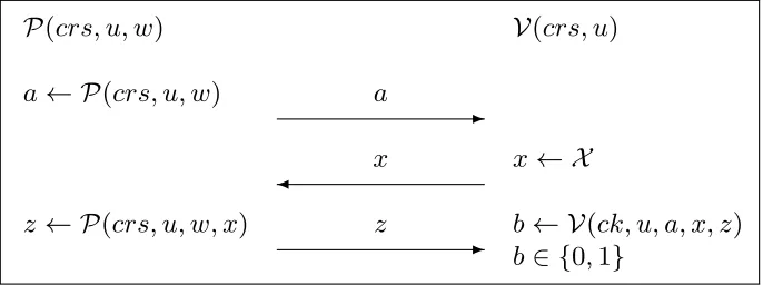
LetRbe a polynomial-time decidable relation. We callwa witness for state-mentuif (crs, u, w)∈R. AΣ-protocol forRis a collection of stateful probabilis-tic polynomial time algorithms (G,P,V). The algorithm G provides a common reference string (which in our paper will be a commitment key as described above). Algorithms P,V function as shown in Figure 2. The challenge spaceX
is implicitly given by the common reference string. Intuitively, V outputs 1 if accepting the proof and 0 if rejecting.
P
(
crs, u, w
)
V
(
crs, u
)
a
← P
(
crs, u, w
)
a
-x
x
← X
z
← P
(
crs, u, w, x
)
z
b
← V
(
ck, u, a, x, z
)
-
b
∈ {
0
,
1
}
Fig. 2.A GeneralΣ-Protocol
Algorithms (G,P,V) are a Σ-protocol if they satisfy completeness, special soundness, and special honest verifier zero-knowledge:
Definition 5 (Perfect Completeness). (G,P,V) is perfectly complete if for all probabilistic polynomial time algorithmsA, we have
Pr
crs← G(1λ); (u, w)← A(crs);a← P(crs, u, w);x← X;z← P(x) : (crs, u, w)∈/R orV(crs, u, a, x, z) = 1
= 1
with the same initial messagea and distinct challenges to compute the witness. For all probabilistic polynomial time algorithmsA
Pr
crs← G(1λ); (u, a, x1, z1, . . . , x
n, zn)← A(crs);
w←χ(u, a, x1, z1, . . . , xn, zn) :
(crs, u, w)∈R or∃i∈[n]such that V(crs, u, a, xi, zi)6= 1
≈1,
where the adversary outputs distinctx1, . . . , xn.
If the above holds with equality, then we say that (G,P,V) has perfect n -special soundness.
Definition 7 (Special Honest Verifier Zero Knowledge (SHVZK)).We say that (G,P,V) has SHVZK if there exists a probabilistic polynomial time simulatorS such that for all interactive probabilistic polynomial time algorithms
A
Pr
crs← G(1λ); (u, w, x)← A(crs);a← P(crs, u, w);z← P(x) :A(crs, a, z) = 1
≈Pr
crs← G(1λ); (u, w, x)← A(crs); (a, z)← S(crs, u, x) :A(crs, a, z) = 1
If the above holds with equality, then we say that(G,P,V)has perfect SHVZK.
Full zero-knowledge. In real life applications special honest verifier zero-knowledge may not suffice since a malicious verifier may give non-random chal-lenges. However, it is easy to convert an SHVZK argument into a full zero-knowledge argument secure against arbitraryverifiers in the common reference string model using standard techniques. The conversion can be very efficient and only costs a small additive overhead. Details of conversion methods can be found in [27,24,20].
2.4 Relations
In this section, we describe the relations for our zero-knowledge proofs. The prover’s witness is a secret vectorasatisfying some conditions, and an opening to a commitment Cwhich is computed froma.
This type of relation could be modelled using a relation with a polynomialP to impose conditions ona, and another polynomial Qto compute the opening toC. The value ris the randomness used to make the commitment.
P(a) =0, C= Com(Q(a);r)
For example,a= (a0, a1, a2) could be a secret vector of bits, imposed byP(a) =
a◦(1−a), andQ(a) =a0+ 2a1+ 4a2 could compute the integer represented
by the bits.
can recover the range proof above by usingb= (1,2,4). We can also get relations about other knapsacks by using a different value ofb.
More formally, letP(a,b),Q(a,b) be length`P, `Qvectors of polynomials of degreesdP, dQrespectively. LetCbe a commitment. Letb∈Z`b
p be a public vec-tor of field elements. The prover gives a zero-knowledge argument of knowledge ofa∈Z`a
p andr∈Zp such that
P(a,b) =0, C= Com(Q(a,b);r)
We give more general batched proofs which can handle tinstances at once. LetC1, . . . , Cmbe commitments. Lett=mn. Letb1,1, . . . ,bm,n∈Z`bp be public vectors of field elements. Thebi,j values allow a single instance to capture some variation in the statement. The batched argument is an argument of knowledge of values{ai,j}m,ni,j=1 and{ri}mi=1, such thatP(ai,j,bi,j) =0fori∈[m], j∈[n], and the prover knows commitment openings
C1 = Com(Q(a1,1,b1,1), Q(a1,2,b1,2), . . . ,Q(a1,n,b1,n); r1)
C2 = Com(Q(a2,1,b2,1), Q(a2,2,b2,2), . . . ,Q(a2,n,b2,n); r2) ..
.
Cm= Com(Q(am,1,bm,1),Q(am,2,bm,2), . . . ,Q(am,n,bm,n);rm)
Whenm=n= 1, we havet= 1 and recover the relation for a zero-knowledge argument of knowledge for a single instance.
The idea is thatQallows the prover to prove things about parts of the wit-ness that were included as commitments in the statement for the zero-knowledge proof. Then P deals with parts of the witness that were not included as com-mitments in the statement. Therefore, by choosingP andQ appropriately, we can easily deal with applications where the evaluation of a polynomial is known, and applications where it is in committed form.
We can easily generalise to the case where multiple polynomialsQ1(a,b), . . . ,Qk(a,b) are given in separate commitments.
2.5 Lagrange Polynomials
Letz1, . . . , zmbe distinct points in some field. The Lagrange polynomialsl1(X), . . . , lm(X) are the unique polynomials of degreem−1 such thatli(zj) =δi,j, whereδi,j is
the Kronecker-delta. In cryptography, Lagrange polynomials have been used for secret-sharing [45].
Forj ∈[m],lj(X) can be computed as
`j(X) := Y
0≤m≤k m6=j
X−zm
zj−zm
=(X−z0) (zj−z0)
· · ·(X−zj−1)
(zj−zj−1)
(X−zj+1)
(zj−zj+1)
· · ·(X−zk)
3
Polynomial commitment schemes
We present a protocol which allows a prover to commit to a polynomial in the discrete-logarithm setting, using a homomorphic commitment scheme. The prover may then later reveal to the verifier an evaluation of the polynomial in a specific pointxchosen by the verifier and prove the evaluation is correct. Bootle et al. [7] dealt with a similar problem for Laurent polynomials with constant term zero, whose coefficients were single field elements. We use the same techniques and generalise to the case of vector coefficients. We treat only positive powers and ignore the condition on the constant term since this suffices for our needs. However, the case of Laurent polynomials is straightforward and similar to [7].
3.1 Definition
A polynomial commitment scheme (Gen,PolyCommit,PolyEval,PolyVerify) en-ables a prover to commit to a secret vector of polynomialsh(X)∈Zlp[X] of some known degree N. Later on the prover may choose to evaluate the committed polynomial in a pointx∈Zp and send an opening to the verifier.
Gen(1λ)→ck: Gen is a probabilistic polynomial time algorithm that returns a commitment key ck. The commitment key specifies among other things a primepof size |p|=λ.
PolyCommit(ck,h(X))→(msg1,st): PolyCommit is a probabilistic polynomial time algorithm that given a commitment keyck and a vector of degree N
polynomials returns a commitment messagemsg1 and a statest.
PolyEval(st, x)→msg2: PolyEval is a deterministic polynomial time algorithm that given a state and a pointx∈Zp returns an evaluation messagemsg2.
PolyVerify(ck,msg1,msg2, x)→h:¯ PolyVerify is a deterministic polynomial time
algorithm that given a commitment key, a commitment message, an evalu-ation message and a point x ∈ Zp returns ⊥ if it rejects the input, or a purported evaluation of the committed vector of polynomials inx.
A polynomial commitment scheme should be complete, (m+ 1)-special sound and special honest verifier zero-knowledge as defined below.
The definition of completeness simply guarantees that if PolyCommit and PolyVerify are carried out honestly, then PolyVerify will return the correct poly-nomial evaluationh(x).
Definition 8 (Perfect Completeness).
(Gen,PolyCommit,PolyEval,PolyVerify) has perfect completeness if for all
λ∈N, for allck←Gen(1λ), and allh(X)∈
Zlp[X]of degree N, and allx∈Zp
Pr
(msg1,st)←PolyCommit(ck,h(X))
msg2←PolyEval(st, x) ¯
h←PolyVerify(ck,msg1,msg2, x)
: ¯h=h(x)
The definition of (m+ 1)-Special Soundness guarantees that given m+ 1 accepting evaluations for different evaluation points, but from the same poly-nomial commitment message msg1, then it is possible to extract a polynomial h(X) that is consistent with the evaluations produced. Furthermore, any other accepting evaluations for the same commitment will also be evaluations ofh(X).
Definition 9 (Computational (m+ 1)-Special Soundness).
(Gen,PolyCommit,PolyEval,PolyVerify)is(m+1)-special sound if there ex-ists a probabilistic polynomial time algorithm χthat uses m+ 1accepting tran-scripts with the same commitment messagemsg1to compute the committed poly-nomialh(X). For all probabilistic polynomial time adversariesAand allL≥m
Pr
ck←Gen(1λ) (msg1, x(0),msg(0)
2 , . . . , x(L),msg (L)
2 )← A(ck)
h(X)←χ(ck,msg1, x(0),msg(0)
2 , . . . , x(m),msg (m) 2 )
¯
hi←PolyVerify(ck,msg1,msg (i) 2 , x(i))
: There is a ¯ hi =⊥ or all h¯i=h(x(i))
≈1,
where the adversary outputs distinct pointsx(0), . . . , x(L)∈
Zp and the extractor returns a degreeN vector of polynomials.
Perfect special honest verifier zero-knowledge means that given any evalua-tion point xand an evaluation h(x), it is possible to simulatemsg1,msg2 that are distributed exactly as in a real execution of the protocol, in a way that is consistent with the evaluationh(x).
Definition 10 (Perfect Special Honest Verifier Zero Knowledge). (Gen,PolyCommit,PolyEval,PolyVerify) has perfect special honest verifier zero knowledge (SHVZK)if there exists a probabilistic polynomial time simulator
S such that for all stateful probabilistic polynomial time adversariesA
Pr
ck←Gen(1λ); (h(X), x)← A(ck) (msg1,st)←PolyCommit(ck,h(X))
msg2←PolyEval(st, x)
: A(msg1,msg2) = 1
= Pr
ck←Gen(1λ); (h(X), x)← A(ck)
(msg1,msg2)← S(ck, x,h(x)) : A(msg1,msg2) = 1
3.2 Construction
In the following, we will build a polynomial commitment scheme on top of a perfectly-hiding, homomorphic commitment scheme (Gen,Com) to vectors in Znlp . Let us first give some intuition about how the construction will work.
Leth(X) =PNi=0hiXi be a polynomial of degree N = (n+ 1)m−1 with coefficients that are row-vectors inZl
p. Define anm×(n+ 1)lmatrix
h0,0 h0,1 · · · h0,n h1,0 h1,1 · · · h1,n ..
. ... . ..
hm−1,0hm−1,1· · · hm−1,n =
h0 hm · · · hnm h1 hm+1 · · · hnm+1
..
. ... . .. hm−1h2m−1· · · hN
With this matrix we haveh(X) =Pnj=0(Pmi=0−1hi,jXi)Xmj. In the polyno-mial commitment scheme, the prover commits to each row of the matrix with commitments {Hi}mi=0−1. After receiving a pointx from the verifier, the prover
computes for each column ¯hj = Pmi=0hi,jxi and sends them to the verifier as part of openings of the commitmentQmi=0−1Hxi
i . The verifier can use the homo-morphic property of the commitments to check that the ¯hj values are correctly formed and computeh(x) =Pnj=0h¯jxjm.
While the main idea we have sketched above gives the verifier assurance that the committed polynomial has been correctly evaluated, the prover may not be happy. The problem is that the solution gives away information about the coefficients ofh(X). We will therefore introduce some random blinding vectors to ensure no information is leaked about the committed coefficients except the evaluation of the polynomial. We will also adjust the protocol to handle an arbitrary polynomial degree N =mn+d for 0 ≤ d < m by shifting the first column of the matrix.
We pick random blindersb1, . . . ,bn ←Zpl and define an (m+ 1)×(n+ 1)l matrix{hi,j}
m,n
i=0,j=0 as follows:
h0 b1 · · · bn−1 bn
h1 hd+1 · · · h(n−2)m+d+1 h(n−1)m+d+1
.. .
hd−b1 ... . .. hnm
0 hnm+1
..
. ...
0 hm+d−1 · · · h(n−2)m+d−1 hN−1
0 hm+d−b2· · · h(n−2)m+d−bnhN
We can therefore rewrite the polynomial as
h(X) = m X
i=0
hi,0Xi+ n X j=1 m X i=0
hi,jXi !
X(j−1)m+d.
In the polynomial commitment scheme, the prover commits to each row of the matrix with commitments {Hi}mi=0. After receiving a point xfrom the verifier,
the prover computes for each column ¯hj = Pm
i=0hi,jxi and sends them to the verifier as part of an opening of the commitment Qmi=0Hxi
i . The verifier can use the opening to check that the ¯hj values are correct and compute h(x) = ¯
h0+Pnj=1h¯jx(j−1)m+d. We describe the full polynomial commitment scheme below.
PolyCommit(ck,h(X))→(msg1,st): The prover randomly selectsb1, . . . ,bn← Zlpand arranges them into a matrix with entries {hi,j}
m,n
i=0,j=0 as follows:
h0 b1 · · · bn−1 bn
h1 hd+1 · · · h(n−2)m+d+1 h(n−1)m+d+1
.. .
hd−b1 ... . .. bn
0 hnm+1
..
. ...
0 hm+d−1 · · · h(n−2)m+d−1 hN−1
0 hm+d−b2· · · h(n−2)m+d−bnhN
For 0 ≤ i ≤ m, the prover randomly selects ri ← Zp and computes a commitmentHi to theith row of the matrix using randomnessri.
msg1= ({Hi}mi=0), st= h(X),{bj}nj=1,{ri}mi=0
The prover sendsmsg1to the verifier.
PolyEval(st, x): →(msg2): For 0≤j≤n, the prover computes
¯ hj=
m X
i=0
hi,jxi+1.
The prover also computes ¯r=Pmi=0rixi. Setmsg2= {h¯j}nj=0,r¯
.
The prover sendsmsg2to the verifier.
PolyVerify(ck,msg1,msg2, x): →(cmt): The verifier checks whether
com(¯h0, . . . ,h¯n; ¯r) = m Y
i=0 Hixi.
Return⊥if this fails.
After accepting the commitment opening, the verifier returns
¯ h=
m X
i=0
hi,0xi+ n X j=1 m X i=0
hi,jxi !
x(j−1)m+d.
Lemma 1. The polynomial commitment protocol given above has perfect com-pleteness, computational (m+ 1)-special-soundness, and perfect special honest verifier zero-knowledge.
Givenxandh(x), we describe an efficient simulator to prove special honest verifier zero knowledge. The simulator first picks random ¯h1, . . . ,h¯n ←Zlp and then computes ¯h0=h(x)−
Pn
j=1h¯jx(j−1)m+d. In other words, thehjare chosen uniformly at random, conditional on giving the correct evaluation h(x). The simulator also picks at random ¯r ∈ Zp and r1, . . . , rm ← Zp and sets Hi = Comck(0;ri). Finally, it computesH0= Comck(¯h0, . . . ,h¯n; ¯r)
Qm i=1H
−xi i . This is a perfect SHVZK simulation. First, because the commitment scheme is perfectly hiding, the commitmentsH1, . . . , Hmare identically distributed in real proofs and simulated proofs. The values ¯h1, . . . ,h¯n and ¯rare also independently and uniformly at random in real proofs due to the choices ofb1, . . . ,bn andr0, just as in the simulated proofs. Finally, given these random values both real and simulated proofs, the matchingH0and ¯h0are uniquely determined. This means
we have identical distributions of real and simulated proofs which are consistent with the evaluationh(x).
Finally, we prove (m+ 1)-special soundness. Suppose that we are givenmsg1
andx(0), . . . , x(m),msg(0)2 , . . . ,msg(2m)which are all accepting, and where thex(i)
are distinct. Consider the Vandermonde matrix:
1 1 · · · 1
x(0) x(1) · · · x(m)
..
. ... . .. ...
x(0)m
x(1)m
· · · x(m)m
This matrix is invertible, meaning that for any 0≤k≤m, we can take linear combinations of the columns to obtain (0, . . . ,0,1,0, . . . ,0)T, where thekth entry is 1. We may take the same linear combinations of the verification equation com(¯h0, . . . ,h¯n; ¯r) =
Qm i=0H
xi
i in order to find openings to each Hk. We now have that H0, . . . , Hm are commitments to known row vectors (hi,0, . . . ,hi,n) with known randomness ri. We define the extracted vector of polynomials to be h(X) =Pmi=0hi,0Xi+Pnj=1 Pmi=0hi,jXiX(j−1)m+d, which is a vector of degreeN polynomials.
By the binding property of the commitment scheme, for each accepting tran-script, we have
¯ hk=
m X
i=0
hi,0(x(k))i+
n X
j=1
m X
i=0
hi,j(x(k))i !
(x(k))(j−1)m+d.
Therefore, all openings are consistent with the extracted polynomialh(X). ut
Communication. The prover must sendm+ 1 group elements andl(n+ 1) + 1 field elements to the verifier.
4
Batch Protocol for Low Degree Relations
We give an argument of knowledge of values{ai,j}i∈[m],j∈[n] and{ri}i∈[m], such
that P(ai,j,bi,j) = 0 for i ∈ [m], j ∈ [n], and the prover knows commitment openings
C1 = com(Q(a1,1,b1,1), Q(a1,2,b1,2), . . . ,Q(a1,n,b1,n); r1) C2 = com(Q(a2,1,b2,1), Q(a2,2,b2,2), . . . ,Q(a2,n,b2,n); r2)
.. .
Cm= com(Q(am,1,bm,1),Q(am,2,bm,2), . . . ,Q(am,n,bm,n);rm)
The protocol we design will be more efficient than repeatingt=mninstances of the basic protocol in parallel, as the communication depends on√trather than
t.
In the following we will refer to the parameters`a, `b, `P, dP, `Q, dQsuch that ai,j∈Z`a
p , bi,j ∈Z`b
p,Pis a vector of `P (`a+`b)-variate polynomials of total degreedP, and Qis a vector of`Q (`a+`b)-variate polynomials of total degree
dQ.
4.1 Intuition behind Protocol
The protocol embeds multiple instances of the same polynomial equality into a single polynomial by using Lagrange interpolation polynomials, inspired by [26,1]. To recover a single instance, simply evaluate the polynomial in one of the interpolation points.
More concretely, letz1, . . . , zmbe distinct points inZp, and letl1(X), . . . , lm(X) be their associated Lagrange polynomials such that li(zj) = δi,j. Let l0(X) = Qm
i=1(X−zi). The prover produces the following commitments.
A0 = com(a0,1, a0,2, . . . ,a0,n ;r0 )
A1 = com(a1,1, a1,2, . . . ,a1,n ;r1 )
A2 = com(a2,1, a2,2, . . . ,a2,n ;r2 ) ..
.
Am= com(am,1,am,2, . . . ,am,n;rm)
Here, the values a0,1, . . . ,a0,n∈Zla
p, where the value of the first index is 0, are blinding values chosen uniformly at random. These are completely unrelated to the values of the witness, which are a1,1, . . . ,am,n, where the first index has a value strictly greater than 0. After receiving a random challenge xfrom the verifier, the prover sends ¯aj =
Pm
i=0ai,jli(x) to the verifier for eachj ∈[n]. The verifier now checks the received ¯aj against the commitments Ai. This proves knowledge of theavalues. It remains to demonstrate thatai,j,bi,jsatisfy the polynomial relations in the statement. Let ¯bj=
Pm
original polynomial,P(ai,j,bi,j). This implies, for example, thatP(¯aj,b¯j)≡0 modl0(x), or in other words, that P(¯aj,b¯j) is a multiple ofl0(X) for each j.
The prover must commit to the coefficients ofP(¯aj,b¯j)/l0(x) in advance (as a
polynomial in x), and uses the polynomial commitment scheme to achieve this for everyj simultaneously.
Finally, the prover needs to convince the verifier that the commitmentsCi contain commitments toQ(ai,j,bi,j). This is done in a similar way to theP poly-nomial, except here we build up polynomial equalities over committed values. The full protocol can be found below.
Common Reference String: crs= (ck, z1, . . . , zm) whereck←Gen(1λ) and
z1, . . . , zmare distinct points inZpdefining Lagrange polynomialsl1(X), . . . , lm(X) such thatli(zj) =δi,j and definingl0(X) =
Qm
j=1(X−zj). Statement: {Ci}i∈[m],{bi,j}i∈[m],j∈[n],P,Qpolynomials.
Prover’s Witness: {ai,j}i∈[m],j∈[n],{ri}i∈[m] such that
P(ai,j,bi,j) =0fori∈[m], j∈[n]
Ci= com(Q(ai,1,bi,1),Q(ai,2,bi,2), . . . ,Q(ai,n,bi,n);ri) fori∈[m]
P →V: Pick r0, s0, . . . , sm ← Zp and a0,1, . . . ,a0,n ← Z`ap and c1, . . . ,cn ←
Z`Qp . Compute
C0= Comck(c1, . . . ,cn;r0) and Ai= Comck(ai,1, . . . ,ai,n;si) fori∈ {0}∪[m].
Define
¯ aj(X) =
Pm
i=0ai,jli(X) b¯j(X) = Pm
i=1bi,jli(X)
P∗j(X) =P(¯aj(X),b¯j(X))
l0(X) Q
∗
j(X) =cj+
Pm
i=1Q(ai,j,bi,j)li(X)−Q(¯aj(X),b¯j(X)) l0(X)
Run PolyCommit(ck, P∗j(X)
j∈[n])→(msgP,1,stP).
Run PolyCommit(ck, Q∗j(X)
j∈[n])→(msgQ,1,stQ).
The prover sends{Ai}i∈[m] andmsgP,1,msgQ,1 to the verifier.
P ←V: Send the challengex←Zp\ {z1, . . . , zm}to the prover. P →V: Run
PolyEval(stP, x)→msgP,2 PolyEval(stQ, x)→msgQ,2.
Compute
¯
aj = ¯aj(x) r¯= m X
i=0
rili(x) ¯s= m X
i=0 sili(x).
V: Run
PolyVerify(ck,msgP,1,msgP,2, x)→p¯ = (¯p1, . . . ,p¯n)
and
PolyVerify(ck,msgQ,1,msgQ,2, x)→q¯= (¯q1, . . . ,q¯n).
Return 0 if ¯p=⊥or ¯q=⊥. Check
Comck(¯a1, . . . ,¯an; ¯s) = m Y
i=0 Alii(x).
Compute ¯bj= ¯bj(x) and check for allj∈[n] that
P(¯aj,b¯j) = ¯pjl0(x).
Check that
Comck(
¯
qjl0(x) +Q(¯aj,b¯j) j∈[n]; ¯r) = m Y
i=0 Cili(x).
If all checks are satisfied, then the verifier outputs 1, and otherwise 0.
Lemma 2. The batch protocol has perfect completeness, ms-special-soundness, and perfect special honest verifier zero-knowledge, wherems= (mmax(dP, dQ)+ 1).
Proof. Perfect completeness of the protocol follows by perfect completeness of the PolyCommit sub-protocol, and by careful inspection.
For perfect special honest verifier zero knowledge, we provide an efficient simulator for the protocol. The simulator selects z1, . . . , zm as the prover. She then selects ¯aj ← Z`ap , ¯r,s¯ ← Zp, ¯qj ← Z`Qp , and A1, . . . , Am as uniformly random commitments to 0. All these values are distributed exactly as in a real protocol, where they are also uniformly random.
She then simulates the polynomial commitment and evaluation messages
msgP,1,msgP,2,msgQ,1,msgQ,2 using the evaluation point x and evaluations ¯p and ¯q, which are determined by the values already simulated. By the perfect SHVZK of the polynomial commitment scheme, the simulated values have iden-tical distribution to the real proofs. Furthermore, since the polynomial commit-ment simulator takes the polynomial evaluation as input, the simulated poly-nomial commitments are consistent with the rest of the simulated values in the outer protocol.
In both the real and simulated protocols, the verification equations now deter-mine the values ofA0andC0uniquely, and the simulator can easily compute the correct values by rearranging the equations. The entire simulated proof therefore has the same distribution as a real proof.
Pick anym+ 1 of the challenges, and note that the matrix
M =
l0(x(1)) l1(x(1)) · · · lm(x(1))
l0(x(2)) l1(x(2)) · · · l
m(x(2)) ..
. ... . .. ...
l0(x(m+1))l1(x(m+1))· · · lm(x(m+1))
is invertible. This follows from linear independence of the polynomialsl0(X), . . . , lm(X). If the determinant was zero, there would be a non-trivial linear dependence between the columns of the matrix. This would give a non-trival dependence relation between the polynomials.
Therefore, for eachi, it is possible to take a linear combination of the rows to produce (0, . . . ,0,1,0, . . . ,0), where the 1 is at theith entry. By taking the same linear combinations of the left and right hand sides of the verification equation Comck(¯a1, . . . ,¯an; ¯s) =
Qm i=0A
li(x)
i for m+ 1 different transcripts, we can for eachi ∈ {0} ∪[m] extract an opening {ai,j}j∈[n] and si ofAi. By the binding property of the commitment scheme, we now have in each transcript that ¯aj is correctly formed as a polynomial determined by the openings of theAievaluated in x.
By the special soundness of the polynomial commitment protocols, we extract polynomialsP∗j(X) of degree (dP−1)m, and Q∗j(X) of degree (dQ−1)msuch that in each transcript, ¯pj =P∗j(x) and ¯q=Q∗j(x) for the challengexappearing in that transcript.
Consider the verification equationsP(¯aj,b¯j) = ¯pjl0(x). By the binding prop-erty of the commitment scheme, we have that P(¯aj(x),b¯j(x)) = P∗j(x)l0(x) holds for ms different challenges x. Since ms is larger than the degree of the polynomial this implies that we have an equality of polynomials. By evaluating the polynomial expression at a particular interpolation pointzi, and parsing the resulting vector correctly, we see thatP(ai,j,bi,j) =P∗j(zi)l0(zi) =0 for each
i, j.
We can in a similar manner to the extraction of theAi extract openings of allCi to valuesci,1, . . . ,ci,n. The last verification equation tells us that for each
j∈[n]
¯
qjl0(x) +Q(¯aj,b¯j) = m X
i=0
ci,jli(x).
Sincems is larger than the degree of the polynomials this implies that we have an equality of polynomials. By plugging in the evaluation points zi, we get Q(ai,j,bi,j) =ci,j for eachi∈[m], j∈[n]. ut
Communication Letk1, k2 be the dimensions of the matrix used in the
Poly-Commit subprotocol when committing to P∗, and similarly, let t1, t2 be the
dimensions of the matrix in the subprotocol for committing to Q∗. The to-tal communication cost of the protocol is m+k1+t1+ 4 group elements and
Single Proof Case Whent=mn= 1 and the prover is proving a single relation, we may choose parameters so that the protocol only uses a constant number of group elements. Setk1=t1= 1,k2=dP−1,t2=dQ−1. Then the protocol has communication costs of 7 group elements plus`a+`PdP+`QdQ+4 field elements. This minimises communication in the case where the protocol is instantiated over a multiplicative subgroup of a finite field, where group elements are much bigger than field elements.
In the case where the protocol is instantiated using an elliptic curve group, group elements and field elements have roughly the same size. Then, we can
minimise the total communication costs by choosing k2 =
lq dP `P
m
, k1 ≈ dkP2.
Set t2 =lqdQ `Q
m
, t1 ≈ dQ
t2. Then the protocol has costs
√
`PdP + p
`QdQ+ 5
group elements and`a+
√
`PdP+p`QdQ+ 4 field elements.
Batch Proof Case Whent is large, we choose parameters so that the communi-cation costs are proportional to√trather thant. Setk2=lqdP` m
Pn m
,k1≈ dPm k2 .
Sett2=lqdQm `Qn
m
,t1≈dQm
t2 . Finally, setm≈
√
`at, n≈ mt. Then the protocol
has communication costs of roughly√`at+
√
dP`Pt+ p
dQ`Qtgroup elements and√`at+
√
dP`Pt+ p
dQ`Qtfield elements.
Computation The prover’s computational costs are dominated by
O
`
at log`an
+ `Qn log`Qn
+ `PdPt log`Pnk2
+ `PdPt log`Pnt2
exponentiations. OverZp, the prover must perform
O((`a+`b+`P)tdPlogmdP+ (`a+`b+`Q)tdQlogmdQ) +tdPEvalP+tdQEvalQ
multiplications. Here,EvalP is the cost of evaluatingPonce, and similarly forQ. The vectors of polynomialsP∗(X),Q∗(X) are computed using FFT techniques.
The verifier’s computational costs are dominated by
O
m+` an log(m+`an)
+ m+`Qn log(m+`Qn)
+ k1+`Pnk2 log(k1+`Pnk2)
+ t1+`Qnt2 log(t1+`Qnt2)
exponentiations. OverZp, the verifier must perform
O((`P+`Q)n) +nEvalP+nEvalQ
multiplications.
5
Applications
5.1 Membership Argument with Public List
In membership arguments [11,10], the prover wishes to convince the verifier that a commitment contains one of the values in a given list L = (λ0, . . . , λN−1).
Groth and Kohlweiss [28] give an efficient membership argument, which with minor tweaks fits into our framework. For simplicity, we will in the following assumeN is a power of 2.
Statement: (c, λ0, . . . , λN−1)
Witness: `, rsuch thatc= Comck(λ`;r)
Polynomial Encoding: Letm= log2N and let (l0, . . . , lm−1) be the binary
expansion ofl, satisfyinglj(1−lj) = 0 for 0≤j ≤m−1. Define lj,1 :=lj andlj,0= 1−lj. We have that
N−1
X
i=0 λi
m−1
Y
j=0
lj,ij =λl
where we write the binary expansion ofias (i0, . . . , im−1).
Parameter Choice: Writing◦ for the entry-wise product of two vectors – `a = log2N, `b=N, `P = log2N, dP = 2, `Q= 1, dQ= log2N
– a= (l0, . . . , lm−1)
– b= (λ0, . . . , λN−1)
– P(a,b) =a◦(1−a) – Q(a,b) =PNi=0−1λi
Qm−1
j=0 lj,ij
An alternative construction was given in [6] that optimises the membership argument by using ann-ary representation ofl. This alternative construction is captured by our framework as follows, this time assuming for simplicity thatN
is a power ofn, using different polynomials PandQ.
Polynomial Encoding: Letm= lognN and let (l0, . . . , lm−1) be the n-ary
expansion ofl. Letδrs be the Kronecker delta symbol, which is equal to 1 ifr=s and 0 otherwise. Consider the bit-string (δl0,0, δl0,1, . . . , δlm−1,n−1),
each element satisfyingδi,j(1−δi,j) = 0, and with Pn−1
i=0 δlj,i = 1 for each
j. As described in [6], we have that
N−1
X
i=0 λi
m−1
Y
j=0
δj,ij =λl
whereij thejthn-ary digit ofi. Parameter Choice:
– `a =nlognN,`b=N,`P =nlognN,dP = 2,`Q= 1, dQ= lognN – a= (δl0,1, . . . , δlm−1,n−1), not including δj,0for anyj.
– b= (λ0, . . . , λN−1).
– δlj,0= 1− Pn−1
i=1 δlj,ifor eachj. – v= δl0,0, . . . , δlm−1,n−1
– P(a,b) =v◦(1−v) – Q(a,b) =PNi=0−1λi
Qm−1
j=0 δj,ij =λl
Whent = 1 and we are aiming for a constant number of group elements, the simple binary version of the argument gives the lowest communication costs. Otherwise, in the cases wheretis large, or wheret= 1 and we aim to minimise the total number of elements communicated, setting n = 3 gives the lowest communication costs. The protocol efficiency is reported in Table 1.
5.2 Polynomial Evaluation Argument
In a polynomial evaluation argument [23,10], we have a polynomial of degree
N and commitments to a point and its purported evaluation in that point. The prover wants to convince the verifier that the committed evaluation of the polynomial is correct.
The most efficient discrete logarithm based polynomial evaluation argument was given by Bayer and Groth [2]. We will now use our framework of polynomial relations to capture their protocol.
Statement: (cu, cv, h(X)), whereh(X) is a polynomial of degreeN.
Witness: u, η, v, νsuch thatcu= Comck(u;η), cv= Comck(v, ν), andh(u) =
v.
Polynomial Encoding: Setui=u2 i
for 0≤i≤log2N−1, so thatui=u2i−1
for eachi. Ifh(X) =PNi=0−1hiXi, then we can writeh(u) = PN−1
i=0 hiQ
log2N−1
j=0 u
ij j. Parameter Choice:
– `a = log2N, `b=N, `P = log2N−1,dP = 2,`Q= 1, dQ= log2N
– a= (u0, . . . , ulogN−1)
– b= (h0, . . . , hN−1)
– P(a,b) = (u1−u20, . . . , ulogN−1−u2logN−2)
– Q(a,b) =PNi=0−1hiQ
logN−1
j=0 u
ij j
With alternative choices of the matricesP,Q, we can improve the communi-cation costs of their argument by switching to ann-ary encoding of the powers in the polynomial.
Polynomial Encoding: Set ui = un i
for 0 ≤ i ≤ lognN −1, so that
ui = uni−1 for each i. If h(X) =
PN−1
i=0 hiXi, then we can write h(u) = PN−1
i=0 hiQ
lognN−1
j=0 u
ij
j , where this time,ij is the jth digit of thenary rep-resentation ofi. This gives rise to the efficiencies listed in Table 1.
Parameter Choice:
– `a = lognN,`b=N,`P = lognN,dP =n, `Q= 1,dQ = lognN – a= (u0, . . . , ulognN−1)
– b= (h0, . . . , hN−1)
– P(a,b) = (u1−un0, . . . , ulognN−1−u n
lognN−2)
– Q(a,b) =PNi=0−1hiQ
lognN−1 j=0 u
Whent = 1 and we are aiming for a constant number of group elements, setting n = 4 gives the lowest communication costs. When t = 1 and we aim to minimise the total number of elements communicated, we setn= log2N
log2log2N. Otherwise, in the cases wheret is large, settingn= 6 gives the lowest commu-nication costs. The protocol efficiency is reported in Table 1.
We note that [1] gives a batch argument for polynomial evaluation based on similar ideas. However, ours is more communication efficient.
Remark. The relations above arise from choices of a small set of powers of u
which generate all powers from u to uN−1. This is the same as choosing an
additive basis for [N−1]. For certain parameter choices, we have found modest benefits to using more complex bases, such as generalised Zeckendorf bases, but these give only slight improvements, so are omitted for simplicity.
5.3 Range Proof
In range proofs [9,38], we have a commitment and a range [A;B]. The prover wants to convince the verifier that the committed value inside the commitment falls in the given range. A common strategy for constructing a range proof is to write the committed value in binary, prove all the bits are indeed 0 or 1, and that their weighted sum yields a number within the range. We now describe this type of range proof in our framework of polynomial relations, where we for simplicity focus on intervals [0, N] withN = 2m−1.
Statement: (N, c)
Witness: a, r such thatc= Comck(a;r), a∈[0, N].
Polynomial Encoding: Leta0, . . . , am−1 be the binary representation ofa,
so thatai(1−ai) = 0 for 0≤i≤m−1. Thena= Pm−1
i=0 ai2i. Parameter Choice:
– `a =m, `b=m, `P =m, dP = 2, `Q= 1, dQ=m+ 1 – a= (a0, . . . , am−1)
– b= (20,21, . . . ,2m−1)
– P(a,b) =a◦(1−a) – Q(a,b) =Pmi=0−1ai2i
With an alternative choice of P,Q, following [16], it is possible to improve the communication costs of the argument by using ann-ary base. This gives rise to the efficiencies listed in Table 1.
Polynomial Encoding: Let N = nm−1. Let a0, . . . , a
m−1 be the n-ary
representation of a, so that Qnk−=01(ai −k) = 0 for 0 ≤ i ≤ m−1. Then
a=Pmi=0−1aini. Parameter Choice:
– `a =m, `b=m,`P =m,dP =n,`Q = 1,dQ= 1 – a= (a0, . . . , am−1)
– P(a,b) =a◦(a−1)◦. . .(a−n+ 1) – Q(a,b) =Pmi=0−1aini
Whent = 1 and we are aiming for a constant number of group elements, setting n = 4 gives the lowest communication costs. When t = 1 and we aim to minimise the total number of elements communicated, we setn= log2N
log2log2N. Otherwise, in the cases wheret is large, settingn= 6 gives the lowest commu-nication costs. The protocol efficiency is reported in Table 1.
6
Conclusion
We have provided zero-knowledge arguments for simple polynomial relations, relying solely on the discrete logarithm assumption. When we only have one instance of the argument, t = 1, the single value membership arguments and polynomial evaluation arguments compiled within our framework improve on the state of the art both asymptotically and for practical parameters. When there are many instances,t >1, we have a batch argument for polynomial relations, which is significantly more efficient than the na¨ıve solution of repeating single instance arguments many times.
References
1. Stephanie Bayer.Practical zero-knowledge Protocols based on the discrete logarithm Assumption. PhD thesis, University College London, 2014.
2. Stephanie Bayer and Jens Groth. Zero-Knowledge Argument for Polynomial Eval-uation with Application to Blacklists. InEUROCRYPT, pages 646–663, 2013. 3. Mihir Bellare, Juan A. Garay, and Tal Rabin. Batch Verification with Applications
to Cryptography and Checking. InEUROCRYPT, pages 236–250, 1998.
4. Josh Benaloh and Michael de Mare. One-way accumulators: A decentralized alter-native to digital signatures. Advances in CryptologyEUROCRYPT’93, 1994. 5. Jonathan Bootle, Andrea Cerulli, Pyrros Chaidos, Essam Ghadafi, and Jens Groth.
Foundations of Fully Dynamic Group Signatures. InACNS, pages 117–136, 2016. 6. Jonathan Bootle, Andrea Cerulli, Pyrros Chaidos, Essam Ghadafi, Jens Groth, and Christophe Petit. Short Accountable Ring Signatures Based on DDH. In
ESORICS, pages 243–265, 2013.
7. Jonathan Bootle, Andrea Cerulli, Pyrros Chaidos, Jens Groth, and Christophe Petit. Efficient zero-knowledge arguments for arithmetic circuits in the discrete log setting. InEUROCRYPT, pages 327–357, 2016.
8. Jonathan Bootle, Andrea Cerulli, Essam Ghadafi, Jens Groth, Mohammad Ha-jiabadi, and Sune K. Jakobsen. Linear-time zero-knowledge proofs for arith-metic circuit satisfiability. Cryptology ePrint Archive, Report 2017/872, 2017.
http://eprint.iacr.org/2017/872.
9. Fabrice Boudot. Efficient proofs that a committed number lies in an interval. In
EUROCRYPT, pages 431–444, 2002.
11. Emmanuel Bresson and Jacques Stern. Efficient revocation in group signatures. In
PKC, pages 190–206, 2001.
12. Jan Camenisch and Rafik Chaabouni. Efficient protocols for set membership and range proofs. Advances in Cryptology-ASIACRYPT . . ., 2008.
13. Jan Camenisch, Markulf Kohlweiss, and Claudio Soriente. An accumulator based on bilinear maps and efficient revocation for anonymous credentials. Public Key CryptographyPKC . . ., 2009.
14. Jan Camenisch and Anna Lysyanskaya. Dynamic accumulators and application to efficient revocation of anonymous credentials. InCRYPTO, pages 61–76, 2002. 15. Jan Camenisch and Markus Stadler. Proof systems for general statements about
discrete logarithms. Technical Report 260, ETH Zurich, 1997.
16. Rafik Chaabouni, Helger Lipmaa, and Abhi Shelat. Additive combinatorics and discrete logarithm based range protocols. In ACISP, volume LNCS 6168, pages 336–351, 2010.
17. Geoffroy Couteau, Thomas Peters, and David Pointcheval. Removing the strong RSA assumption from arguments over the integers. In Advances in Cryptology -EUROCRYPT 2017 - 36th Annual International Conference on the Theory and Applications of Cryptographic Techniques, Paris, France, April 30 - May 4, 2017, Proceedings, Part II, pages 321–350, 2017.
18. Ronald Cramer and Ivan Damg˚ard. Zero-knowledge proofs for finite field arith-metic, or: Can zero-knowledge be for free? InCRYPTO, pages 424–441, 1998. 19. Ronald Cramer, Ivan Damg˚ard, and Berry Schoenmakers. Proofs of partial
knowl-edge and simplified design of witness hiding protocols.Advances in Cryptology . . ., 839:174–187, 1994.
20. Ivan Damg˚ard. Efficient concurrent zero-knowledge in the auxiliary string model. InEUROCRYPT, pages 418–430, 2000.
21. Ivan Damg˚ard and Nikos Triandopoulos. Supporting Non-membership Proofs with Bilinear-map Accumulators. IACR ePrint archive report 538, 2008.
22. Prastudy Fauzi, Helger Lipmaa, and Bingsheng Zhang. Efficient Non-Interactive Zero Knowledge Arguments for Set Operations. In Financial Cryptography and Data Security, pages 216–233, 2014.
23. Eiichiro Fujisaki and Tatsuaki Okamoto. Statistical zero knowledge protocols to prove modular polynomial relations. InCRYPTO, pages 16–30, 1997.
24. Juan A. Garay, Philip MacKenzie, and Ke Yang. Strengthening zero-knowledge protocols using signatures. Journal of Cryptology, 2006.
25. Roario Gennaro, Darren Leigh, Ravi Sundaram, and William Yerazunis. Batching Schnorr identification scheme with applications to privacy-preserving authorization and low-bandwidth communication devices. InASIACRYPT, volume LNCS 3329, pages 276–292, 2004.
26. Rosario Gennaro, Craig Gentry, Bryan Parno, and Mariana Raykova. Quadratic Span Programs and Succinct NIZKs without PCPs. InEUROCRYPT, pages 626– 645, 2013.
27. Jens Groth.Honest verifier zero-knowledge arguments applied. PhD thesis, Aarhus University, 2004.
28. Jens Groth and Markulf Kohlweiss. One-out-of-Many Proofs: Or How to Leak a Secret and Spend a Coin. InEUROCRYPT, pages 253–280, 2015.
29. Ryan Henry and Ian Goldberg. Batch proofs of partial knowledge. InACNS, pages 502–517, 2013.
31. Charanjit Jutla and Arnab Roy. Shorter {Q}uasi-{A}daptive{NIZK} {P}roofs for{L}inear{S}ubspaces. InASIACRYPT, volume LNCS 8269, pages 1–20, 2013. 32. Charanjit S. Jutla and Arnab Roy. Switching lemma for bilinear tests and constant-size NIZK proofs for linear subspaces. Lecture Notes in Computer Science (includ-ing subseries Lecture Notes in Artificial Intelligence and Lecture Notes in Bioin-formatics), 8617 LNCS(PART 2):295–312, 2014.
33. Aniket Kate, Gregory M. Zaverucha, and Ian Goldberg. Constant-size commit-ments to polynomials and their applications. In Advances in Cryptology - ASI-ACRYPT 2010 - 16th International Conference on the Theory and Application of Cryptology and Information Security, Singapore, December 5-9, 2010. Proceedings, pages 177–194, 2010.
34. Joe Kilian. A note on efficient zero-knowledge proofs and arguments. InSTOC, pages 723–732, 1992.
35. Eike Kiltz and Hoeteck Wee. Quasi-adaptive NIZK for linear subspaces revisited.
Lecture Notes in Computer Science (including subseries Lecture Notes in Artificial Intelligence and Lecture Notes in Bioinformatics), 9057(339563):101–128, 2015. 36. Jiangtao Li, Ninghui Li, and Rui Xue. Universal Accumulators with Efficient
Nonmembership Proofs.Proceedings of the 5th international conference on Applied Cryptography and Network Security (ACNS), pages 253–269, 2007.
37. Benoˆıt Libert, Somindu C. Ramanna, and Moti Yung. Functional commitment schemes: From polynomial commitments to pairing-based accumulators from sim-ple assumptions. In43rd International Colloquium on Automata, Languages, and Programming, ICALP 2016, July 11-15, 2016, Rome, Italy, pages 30:1–30:14, 2016. 38. Helger Lipmaa. On diophantine complexity and statistical zero-knowledge
argu-ments. InASIACRYPT, pages 398–415, 2003.
39. Silvio Micali, Michael O. Rabin, and Joe Kilian. Zero-knowledge sets. InFOCS, pages 80–91, 2003.
40. Lan Nguyen. Accumulators from bilinear pairings and applications to ID-based ring signatures and group membership revocation. In CT-RSA, pages 275–292, 2005.
41. Charalampos Papamanthou, Elaine Shi, and Roberto Tamassia. Signatures of correct computation. In Theory of Cryptography - 10th Theory of Cryptography Conference, TCC 2013, Tokyo, Japan, March 3-6, 2013. Proceedings, pages 222– 242, 2013.
42. Torben P. Pedersen. Non-interactive and information-theoretic secure verifiable secret sharing. InCRYPTO, pages 129–140, 1991.
43. Kun Peng. A general, flexible and efficient proof of inclusion and exclusion.Trusted Systems, pages 33–48, 2012.
44. Kun Peng and Feng Bao. Batch ZK Proof and Verification of OR Logic. InInscrypt, volume LNCS 5487, pages 141–156, 2008.
45. Adi Shamir. How to share a secret. Commun. ACM, 22(11):612–613, 1979. 46. Yupeng Zhang, Daniel Genkin, Jonathan Katz, Dimitrios Papadopoulos, and