VICTORIA ~ UNIVERSITY
•
~..
z 0 0
:
DEPARTMENT OF COMPUTER AND
MATHEMATICAL SCIENCES
Markets For Non-Storable Commodities
Barry A
.
Goss and S
.
Gulay Avsar
(55ECON1)
May
,
1995
(AMS
:
90A60)
TECHNICAL REPORT
VICTORIA UNIVERSITY OF TECHNOLOGY
(P 0 BOX 14428) MELBOURNE MAIL CENTRE
MELBOURNE, VICTORIA
,
3000
AUSTRALIA
MARKETS FOR NON-STORABLE COMMODfflES
by
BARRY
A. Goss AND
s.
GULA y A
VSAR"'December 1994
(Preliminary draft: for comment only)
MARKETS FOR NON-STORABLE COMMODfl'IES
by
BARRY
A.
Goss ANDs.
GULA yA
VSAR*ABSTRACT
Published empirical studies of simultaneous rational expectations models of spot and futures markets for non-storable commodities are extremely rare. Indeed, only two countries, the US and Australia, have produced data sets for the study of such markets. This paper develops, and presents estimates of a simultaneous rational expectations model of the live cattle market in Australia, the world's leading beef exporting country. The model contains functional relationships for short hedgers and speculators combined (there is no disaggregation of hedgers' and speculators' commitments in Australian data), long hedgers and speculators, and consumers, and is completed with a spot price equation and market clearing identity. Unit root tests indicate that all variables in the model are stationary, except for consumption of beef and the price of pork, which are 1(1). Cointegration tests suggest that these two variables are not cointegrated. The model is estimated by the instrumental variables method of McCallum, which provides consistent estimates. The estimates of all 15 structural parameters have the expected sign, and all are significant at the five per cent level. In a 34 month post-sample period, the model forecasts the spot and futures prices with per cent RMSE's of 3.6% and 2.1 % respectively, and in forecasting the spot price, the model outperforms conventional benchmarks such as a random walk and an ARIMA model. The model also outperforms a lagged futures price as a predictor of the spot price, thus providing some evidence against the efficient markets hypothesis.
JEL Codes: Gl3 Ql3 G14
*
Monash University and Victoria University ofTechnology, Australia, respectively. Address for correspondence:Barry A. Goss
Economics Department Monash University Clayton, Vic 3168 Australia
MARKETS
FOR NON-STORABLE COMMODITIES
I
INTRODUCTION
The objective of this paper is to develop and present empirical results for a simultaneous,
rational expectations model of the Australian finished live cattle market. Finished live cattle
are non-storable, because they can be kept in their finished condition for a period of six to
eight weeks only. This model employs information from both spot and futures markets. Only
two countries, the United States and Australia, have introduced futures contracts for live
cattle, and hence only these two countries have produced data sets for the estimation of such
models. While studies of the US live cattle market have been made, comprising simultaneous
rational expectations models, none of these studies has been published, as far as the present
authors are aware, and no such study has been made of the Australian market, to the best of
the present authors' knowledge.
Simultaneous theoretical models of the determination of spot and futures prices have
been developed by Peston and Yamey (1960), Stein (1961, 1964), Dewbre (1981) and Kawai
(1983 ), the last of these being specifically for non-storable commodities. Empirical,
simultaneous models of (non-storable) livestock markets, without rational expectations, have
been developed and estimated by Leuthold and Hartmann (1979) and Leuthold and Garcia
( 1992) and others, while empirical, simultaneous models, with rational expectations, for
storable commodities have been developed by Giles et al. (1985), Goss et al. (1992) and
others. This paper extends the work of Peston and Yamey (1960), Giles et al. (1985) and
Goss et al. (1992) to develop a simultaneous model, with rational expectations, of the
International live cattle markets have attracted considerable attention from researchers,
particularly markets in the USA. Leuthold (1972) was reluctant to reject the random walk
hypothesis with US live cattle price data, even though some filter rules yielded profits net of
transaction costs. Leuthold (1974) did not reject the unbiasedness hypothesis, for US live
cattle futures prices as predictors of delivery date spot prices, with lags up to three months
from maturity, but did reject that hypothesis with longer lags. Giles and Goss (1980) obtained
a very similar result with Australian data. Just and Rausser (1981) compared the predictive
performance of various commercial econometric price forecasts with that of the futures price,
for a range of commodities. In the case of live cattle they found that only one commercial
forecast out of five surpassed the futures price, with a three month lag to maturity, whereas
with longer lags several commercial forecasts surpassed the futures price. While Leuthold
and Hartmann (1979) refined the model prediction approach to market efficiency (for hogs),
Leuthold and Garcia (1992) applied this approach to live cattle, and were unable to reject the
ef~cient markets hypothesis. The latter authors also computed the Stein (1986) social loss
measure for cattle and hogs, and found that this measure was smaller for cattle.
Australia, with 22.4 million head of cattle in 1989, is one of the leading beef
producing countries in the world, ranking behind, for example, USA (98m head), Brazil
(130m head) and Argentina (57m head). In Australia, the main producing states are
Queensland, New South Wales and Victoria. In 1989, Australia exported 872,000 tonnes of
beef, or 55.4% of production, making it the world's leading exporter of beef. The main
export markets served are in USA and Japan; indeed 76. 7% of Australia's beef exports goes
to these two countries (see ABARE, 1993).
Although a cattle contract was introduced on the Sydney Futures Exchange in July
1975, this contract, which called for the delivery of carcases, traded thinly. Revisions were
steers every calendar month (28 steers approx.). This revised contract became relatively successful, with average monthly turnover reaching 16,559 contracts in 1981, and 28,007
contracts being traded in March of that year. By 1985, however, average monthly turnover
had fallen to 1190 contracts, and in May 1986 this Trade Steers Contract, as it had become
known, was replaced by a live cattle contract providing for mandatory cash settlement. This
last contract, although retaining I 0,000 kg live weight of cattle as the contract unit, provided that contracts were to be settled at the Live Cattle Indicator price, which is itself an average
of cash prices for specified cattle types at specified locations. Although still quoted on the
Sydney Futures Exchange, trading in the cash settlement contract became thin after the end
of 1988.
The objective of this paper is to develop, present estimates of, and evaluate a
simultaneous, rational expectations model of price determination in the Australian live cattle
market. Section II of this paper discusses the specification of the model, while Section III
discusses the data employed, presents results for tests for unit roots and cointegration, and
discusses the methodology employed for estimation of the model. Results for the intra-sample
period are presented and discussed in Section IV, while Section V discusses post-sample
simulation by the model, compared with various benchmarks. Some conclusions are presented in Section VI.
II
MODEL SPECIFICATION
This model contains four functional relationships and a market clearing identity. The first
equation explains the combined futures market commitments of both short hedgers and short
and a spot price equation, and is completed with a futures market clearing identity.
This structure represents a modification of the original model by Peston and Y amey
( 1960) and of the approach in the empirical models of Giles et al. (1985) and Goss et al.
(1992), to deal with the case of non-storables. The combined nature of the first two equations
arises because Australian futures market data on commitments of traders are not disaggregated
into hedging and speculation components, as are data for Reporting Traders provided by the
Commodity Futures Trading Commission in the USA.
Although the ideas of Working (1953, 1962) on discretionary hedging were developed
for storable commodities, such as grains, his analysis of the motives for hedging is applicable
to the case of non-storables. Two of the major types of hedging distinguished by Working
(1953, 1962) are carrying charge hedging and selective hedging. On the first hypothesis, the
market commitments of short hedgers, who gain from a reduction in the forward premium,
can be expected to vary directly with the current forward premium (futures price less spot
price), and negatively with the expected forward premium. If, on the other hand, short
hedgers are selective hedgers, where a proportion only of their spot market commitments is
hedged, then their futures market commitments would be expected to vary directly with the
current futures price, and negatively with the expected futures price. Preliminary. estimation
for short hedgers in this market, such as beef producers, favoured the latter of these two
hypotheses.
The market commitments of short speculators, who expect the futures price to fall can
be expected to vary directly with the current futures price, and negatively with the expected
futures price and marginal risk premium. This specification is based on the equilibrium
condition for short speculators (see Goss (1972, p. 23)). The traditional view that the
coefficient of the marginal risk premium is negative (e.g. see Kaldor (1953, p. 23) and
in terms of his "hedging pressure theory", that an increase in the risk premium may have a
positive or negative effect on the futures price, and hence on the market commitments of
speculators.
The supply of futures contracts by short hedgers and short speculators combined may
be expected to be a function of the sum of the influences outlined above. The specification
of this function (HSS) is therefore:
(1)
where Pt
=
current futures price;Pt: I
=
rational expectation of the futures price for period (t+
1), formed in periodand
t·
'
rt
=
marginal risk premium;e
It = error term=
constant;e2
> 0 ;e3
< 0 ;e 4
< > 0 ;This specification suggests a predominance of speculative, rather than hedging, elements.
The rational expectations hypothesis, which is employed in this model, originated with
Muth's observation that mean expectations in an industry are as accurate as "elaborate
equation systems" and his suggestion that "rational expectations are the same as the
predictions of the relevant economic theory (Muth, 1961, p. 316). Much has been written on
the assumptions, implications and formation of rational expectations, and summaries of this
literature can be found in Sheffrin (1985), Minford and Peel (1986), Goss (1991) and Goss
deserve to be emphasized. The first of these is that the rational expectations hypothesis
(REH) implies that agents have the particular economic model, under review, in mind in
forming their expectations, so that any test of the REH is a joint test of the expectations
hypothesis and of the appropriateness of the model (Maddock and Carter 1982). The REH
implies, therefore, that the model which agents believe determines returns is the same as the
model driving returns in practice; otherwise abnormal returns would occur (Minford and Peel,
1986, p. 122). Second, the question of the likelihood of agents learning to form rational
expectations may still be open, although some pessimistic notes (e.g. Frydman, 1983) and
some optimistic notes (e.g. Bray and Savin 1986) have been struck. The question of how
agents learn to form rational expectations has been discussed by several authors, including
Blume et al. (1982) who referred to agents using the same forecasting rule for a long period,
and Stein (1986) whose asymptotically rational expectations converge to Muth rational
expectations with repeated sampling. Third, there is experimental evidence on the
convergence of prices to rational expectations equilibrium in futures and asset markets, in the
work of Plott and Sunder (1982), Friedman et al. (1983) and Harrison (1992). It is the view
of the present authors that experimental evidence suggests that a rational expectations
equilibrium can be achieved in a comparatively short time, especially with futures markets
operating. Finally, support for the REH has been found in models of this type for storable
commodities (see Giles et al. (1985), Goss et al. (1992)).
The market commitments of long hedgers, such as meat processors and beef exporters
traditionally, have been regarded as the mirror image of those of short hedgers (e.g. see Stein,
1961 ). We would expect the positions of these agents, therefore, to vary negatively with the
current forward premium, directly with the expected forward premium, and directly with
measures of the market commitments of these agents, such as planned consumption and
nse, can be expected to vary negatively with the current futures price, directly with the
expected futures price, and negatively With the marginal risk premium. The combined
functional relationship for these two groups of agents could be expected to reflect the sum of
these influences. Preliminary estimation suggested that the price spread variables were more
important than the level form price variables, and that the planned change in consumption
should replace the planned level of consumption. This last change is a consequence of the
unit root and cointegration tests reported in Section Ill. The demand function for futures
contracts (HSL ), therefore is
where
=
current spot price;=
rational expectation of the forward premium in (t+l) formed inperiod t;
change in consumption next period, which is a proxy for the
planned change, assumed to be realized;
=
exports in period (t+ I), which is a proxy for planned exports,assumed to be realized;
r,
= marginal risk premium;This specification contains a mixture of hedging and speculative elements, although it does
suggest a predominance of hedging activity. It is, however, consistent with the view that
The demand for live cattle is derived from the demand for dressed beef. The demand
function for live cattle, therefore, can be seen as dependent upon the spot price of live cattle,
parameters of the demand for the end product, and parameters of the supply of other inputs.
In this case, expected real income next period, and the spot prices of two substitute meats,
lamb and pork, have been employed as parameters of the demand for dressed beef. The spot
price of oats, a complementary input with live cattle, is used as a proxy for the supply of
other inputs. The demand for live cattle, therefore, can be expected to vary negatively with
the spot price of live cattle and the price of oats, and directly with expected real income, the
price of lamb and the price of pork. It should be noted that the demand for live cattle and
the price of pork appear in first difference form in this specification, as a consequence of the
unit root and cointegration tests reported in Section Ill. The resulting specification of this
function is
(3)
where
AC,
=
C, - C,_
1=
change in consumption of live cattle in period t.Yt+ 1
=
real income in period (t+ I), used as a proxy for planned realincome;
A/
=
spot price of lamb;p p p .
AA1 =A, - A1_ 1 = change in price of pork in penod t;
A1
°
=
spot price of oats;is specified first, as a direct function of the current futures price, on the ground that changes
in these two prices are expected to be closely correlated. Secondly, it is postulated that the
spot price is negatively related to the number of store cattle in current yardings for sale,
because an increase in yardings can be expected to lead to an increase in the number of
finished live cattle, and hence to a decline in the spot price. The spot price equation is
written as
(4)
where Nt
=
number of cattle in current yardings; and 618 > 0; 619 < 0.This model, with five endogenous variables (HSS, HSL, LiC, P, A) and four equations,
is completed with the futures market clearing identity
(5)
Conventional identification conditions do not apply to linear multi-equation models with
forward rational expectations (Pesaran, 1987, p. 119). The model developed here, however,
fulfils the identification conditions developed by Pesaran (1987, pp. 156-60) for such models.
m
DA TA, UNIT ROOTS, COINTEGRA TION TESTS AND ESTIMATION
Data
The sample period for the results reported in this paper, after allowance for leads and lags,
is 1980(05) to 1985(12), comprising a total of 68 monthly observations; the post-sample
forecast period, again after allowance for leads and lags, is 1986(03) to 1988(12), which is
a total of 34 observations. Data are discussed in this section under the headings "Endogenous
Endogenous Variables
Futures price data (P) are futures prices of live steers, on the median trading day of the month, for a contract two months prior to delivery (the most heavily traded contract), in
Australian cents per kg live weight from the Sydney Futures Exchange Statistical Yearbook 1980-88.
Spot price data (A) for the period 1980(05) to 1986(06), during which time the Trade Steer Contract (deliverable) traded on the SFE, are prices in Australian cents per kg live weight, for "futures type steers", on the median trading day of the month, provided by the
New South Wales Meat Industry Authority. Data on spot prices for the period 1986(07) to 1988(12), when the Live Cattle (cash settlement) Contract replaced the previous contract, are SFE Live Cattle Indicator prices, on the median trading day of the month, in Australian cents per kg live weight, provided by the SFE. The Live Cattle Indicator price is a five day average of cash prices for specified cattle types at specified selling centres. At maturity, positions in the Live Cattle Contract are settled at the Indicator price.
The total supply of, and total demand for futures contracts (HSS
=
HSL) are measured by the open positions (or commitments) of traders, in number of contracts, on the median trading day of the month, for a futures contract two months from maturity. The data oncommitments of traders, therefore, are synchronized with the data on spot and futures prices. Data on consumption (C) are Australian consumption of beef and beef meat products, per quarter, in thousand tonnes, from Australian Bureau of Statistics (ABS) Livestock and
Livestock Products (Catalogue 7221.0). These data were interpolated to monthly observations using the program TRANSF (Wymer 1977).
Exogenous Variables
per month, from ABS Exports, Australia, Monthly Summary Tables (Cat. 5432) and ABS
Exports of Major Commodities and Their Principal Markets (Cat. 5403). Exports of live beef
cattle from Australia are insignificant and are not included.
Real income (Y) is Australian household disposable income per quarter in million
Australian dollars from ABS, divided by the Consumer Price Index (quarterly), also from
ABS. These data were interpolated to monthly observations.
The marginal risk premium (r) is the monthly average 90 day bank accepted bill rate,
in per cent per annum, minus the monthly average 90 day Treasury Bill rate, in per cent per
annum; observations on both these rates are taken from the Reserve Bank of Australia
Statistical Bulletin. This treatment of the risk premium is consistent with Stein (1991, p. 39).
The spot price of lamb (AL) is the monthly average saleyard price, in Australian cents
per kg for lambs (l 6kg to l 9kg) on a dressed weight basis. Similarly, the spot price of pork (AP)
is the monthly average saleyard price, in Australian cents per kg for pigs (60kg to 70kg) on
a dressed weight basis. Observations on both these prices were taken from Australian Meat
and Livestock Corporation, Statistical Review of Livestock and Meat Industries, and ABARE
( 1993 ). The spot price of oats (A 0
) is the monthly average price, in Australian dollars per
tonne, from ABARE Situation and Outlook: Coarse Grains.
The number of cattle in current yardings (N) is the total number per month of beef
cattle in current yardings listed for sale from ABS Livestock and Livestock Products.
UNIT ROOTS AND COINTEGRA TION TESTS
To obtain meaningful estimates of the parameters of the model, it is necessary that the
residuals of the estimating equations are stationary. This condition will be fulfilled if all the
some of these variables are integrated of order I (1) or higher order, this condition will be
fulfilled only if the non-stationary variables are integrated of the same order and are
cointegrated. The first step in this procedure is to determine the order of integration of the
variables in the model.
In the autoregressive representation of the time series
z,
= pZ,_
1 +e,
(6)where Z is an economic variable, pis a real number, and
e,
is NlD (0, a2), ifIp I
< l,Z,
converges to a stationary series as t ~ oo. On the other hand, if p
=
1, there is a single unitroot and Z1 is non-stationary, while if
I
pI
> 1, the series is explosive.Tests of the hypothesis H(p
=
I) in ( 6), and for variations of this model with constantand time trend, were developed by Dickey and Fuller (1979, 1981). Critical values for these
tests are given in Fuller ( 1976) and Dickey and Fuller ( 1981 ). These tests were extended by
Said and Dickey (1984) to accommodate autoregressive processes in
e,
of higher butunknown order. In this latter case the model is augmented by lagged first differences in Z
to render
e,
as NlD (0, a2) , and the hypothesis H(p=
1) is tested by the AugmentedDickey-Fuller Test (ADF).
In this paper the following models were estimated by ordinary least squares (OLS) to
test the hypothesis of a unit root in all endogenous and exogenous variables in the structural
model:
AZ,
=
µ +y Z,_
1 +<j>AZ,_
1 +e,
(7)AZ,
=
µ +y z,_
1 +<j>AZ,_
1 + $2AZ,_
2 +e,
(8)=
(10)where µ = constant;
J3,
Q>, 4>1 , <f>2 , are coefficients to be estimated;e,
is assumed to be NlD(0,
o2).Models (9) and (10) contain a time trend, (7) and (9) contain a single lagged value of
az,,
and (8) and (10) contain two such lagged values.1 In each case, (7) was estimated first, the
other models being estimated as necessary to whiten
e,.
The hypothesis H(p=
1) isaddressed by testing the hypothesis H(y
=
0) in (7) - (10). This is executed by the ADF test,although it is now preferable to refer to critical values ofMacKinnon (1991), which are based
on more replications than the original Dickey-FuHer tables. Calculated ADF statistics,
together with 5 per cent and 10 per cent critical values from MacKinnon ( 1991 ), are provided
in Appendix 1 for all variables in the model. Notwithstanding the low power of these tests
(see Evans and Savin, 1981), it will be seen that for only two variables (consumption of beef
C and the spot price of pork AP) is it not possible to reject the hypothesis of a single unit
root; these tests support the view that all other variables in the model are stationary.2
In equations (I) and ( 4) of this model there are no non-stationary variables, and hence
it can be assumed that the residuals of these equations will be stationary. In equation (2),
there is one non-stationary variable,
C,,..
1 , and in order to render the residuals in (2)stationary, the first difference of this variable is taken. In equation (2), therefore, the planned
consumption proxy employed for long hedgers' commitments is
a c, ...
1 •In equation (3) there are two 1(1) variables only, C, and
At,
all other variables beingvariables may be stationary, i.e. they may be cointegrated, in which case the residuals of (3)
will be stationary. To investigate whether these I(l) variables are cointegrated, the
cointegration test analysed by MacKinnon (1991), which is based on the work of Engle and
Granger (1987), was employed. The Engle-Granger technique is adequate in this case,
because the question of cointegration refers to two variables only. 3 This test requires first that
a relationship between the I (1) variables, such as the following, be estimated by OLS.
(11)
The hypothesis of no cointegration in (11) is addressed by testing the hypothesis that
the series of estimated values of residuals (
u
1) from (11) contains a unit root. To test thehypothesis of a unit root in
ut
the following model was estimated(12)
and the hypothesis H(y
=
0) was tested, using the Augmented Engle-Granger (AEG) test. Asthe information in Appendix 2 shows, this hypothesis is not rejected at the 10 per cent level,
and hence the hypothesis of no cointegration in (I I) is not rejected. Stationarity of the
residuals in the consumption relationship equation (3), therefore, can be achieved by
employing first differences of the two I(I) variables in this equation,
Ct
andAt.
&timation
Full information estimators of simultaneous models with forward rational expectations, while
potentially more efficient, are less robust to specification errors, and are computationally more
demanding than limited information methods (Pesaran, 1987, p. 162). For these reasons the
model presented here is estimated by the instrumental variables (IV) method of McCallum
expectation of an endogenous variable, such as P1: 1 m (1), as a fitted value on the
information set at time
t
(at) compnsmg all exogenous and predetermined variables(including lagged endogenous variables) in the model. That is
Pt:l
=
E ( P1+1 f <P1 ) andpt+l
=
E(P1+1f<P,)
+ 11, (13)where E ( TJ,) = 0 and TJ, is uncorrelated with the variables in <!>,,under rational expectations.
E ( P, + 1 /
$
1 ) is taken to be linear in the elements ofcl>,.
The structural equations can thenbe estimated by IV, and if the residuals of those equations are not serially correlated, this
method will produce consistent estimates. This procedure is discussed in McCallum (1979)
and is summarized in Giles et al. (1985, pp. 754-55). This procedure has been used for
equation (2) in this model. 4
When serial correlation is present, however, a simple autoregressive (AR) correction
with IV estimation will not produce consistent estimates, as Flood and Garber (1980) pointed
out. In this case an AR transformation has been made, and each of the variables in the
transformed equation was regressed on the elements of the relevant information set, using
OLS. The fitted values so obtained were substituted in the transformed equation (see
McCallum (1979, p. 67-68)), and consistent estimates of the parameters in that equation were
obtained by non-linear least squares, using the option LSQ in TSP (Hall et al., 1993). This
method, which is discussed by Cumby et al. (1983), has been employed for equation (1) in
this model.
Equation (3 ), which contains no expectational variables, but does contain an
Equation (4), which agam does not contain any expectational variables but includes an
endogenous regressor, was estimated also by IV, although in this case a correction for first
order serial correlation was necessary. 6
IV
REsULTS: INTRA-SAMPLE PERIOD
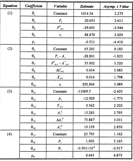
Estimates of the parameters of the model are provided in Table 1, together with their
asymptotic t values. It will be seen that estimates of all 15 structural parameters have the
expected signs and all are significant at the five per cent level (one tail test), thereby
providing strong support for the model specification discussed above. There are, however,
several features of the results for individual equations, which deserve comment. First, the
clear significance of
.
e
3 and6
7 , the coefficients of the expected futures price and expectedprice spread respectively, provides support for the rational expectations hypothesis. Moreover,
the results for equation (1) support the view that HSS is essentially a speculative relationship.
Similarly, the results for equation (2) suggest that commitments on the long side of the market
are a combination of hedging and speculative elements, with a strong discretionary component
in the hedging activities.
Second, the positive estimates of 64 and 610 , the coefficients of the marginal risk
premium in equations (1) and (2) respectively, support an interpretation different from the
Kaldor (1953) - Brennan (1958) view of the risk premium. In equation (1) the positive sign
of
6
4 can be explained as follows: an increase in the marginal risk premium cet par will lead
to an increase in the equilibrium futures price, and hence to an increase in the market
cet par will lead to a decrease in the equilibrium futures price, and hence to an increase in
the market commitments of long speculators. These explanations are similar to the "hedging
pressure theory" of Stein (1986, pp. 48-52), although Stein's argument is directed to the effect
of a change in the risk premium on price alone.
Thirdly, in equation (3), the consumption relationship, the positive sign of
B
14 isconsistent with a substitution relationship between beef and lamb in the sense that a rise in
the price of lamb will lead to an increase in the rate of change of consumption of beef. This
is not the usual sense of substitutability, however, and it is possible that the equilibrium value
of fl Ct, in the period in question, may still be negative. Again, the positive sign of
B
15 ,"".'hich relates a change in the price of pork to a change in the consumption of beef, is
consistent with substitutability between these two meats. This is not the same as the
conventional view of such a relationship, however, because the equilibrium value of
aAt
may be positive while that of .d
Ct
may be negative. Indeed, similar qualifications must beattached to the interpretation of
S
16 , which suggests that live cattle and oats arecomplementary inputs, as well as to the interpretation of the price and income coefficients.
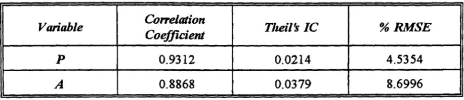
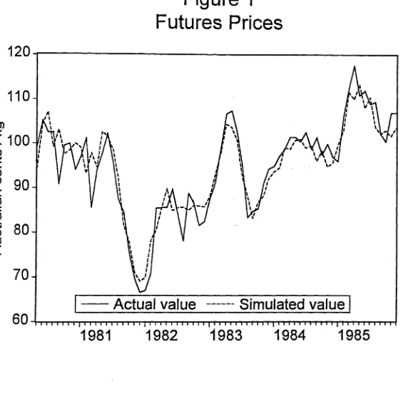
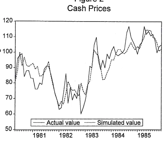
A further test of the appropriateness of this model is the ability of the model to
forecast the endogenous variables within the sample period, according to specified criteria.
Table 2 presents an evaluation of the (static) intra-sample simulation of the two key variables,
P and A, according to the correlation coefficient, Theil's inequality coefficient, and per cent
root mean square error. 7 These simulations are illustrated in figures I and 2. Concentrating
on the per cent RMSE criterion, it will be seen that the better forecast is that of the futures
somewhat larger than those for the futures and spot prices. This may be due, in part, in the
case of fl
ct'
to the inherent difficulty in predicting the magnitudes of first differences, andin the case of HSS (= HSL), to the thinness of the market in the latter part of the sample
period.
v
POST-SAMPLE SIMULATION
A more stringent test of model performance is the ability of the model to forecast key
endogenous variables, against pre-determined criteria, outside the sample period, especially
in comparison with alternative forecasts. Table 3 presents an evaluation of (dynamic) two
months ahead forecasts of the futures and spot prices, for the post-sample forecast period
1986(03) to 1988(12), comprising 34 monthly observations. Concentrating on the per cent
RMSE criterion, it will be seen first, that again the better forecast is that of the futures price,
and second, and more important, the accuracy of both forecasts has improved significantly
compared with the intra-sample simulation of these variables. Indeed, for P and A the per
cent RMSE's are each less than half of their corresponding values for intra-sample simulation.
This latter outcome provides substantial support for the validity of the model.
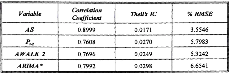
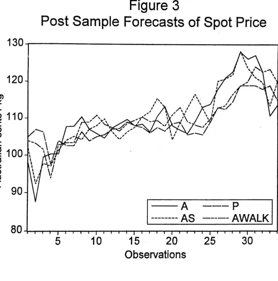
The question is then how does the model perform, compared with alternative price
forecasts. Table 4 presents an evaluation of post-sample fore·casts of the spot pric·e, two
months ahead, by the model (AS: the same as A in Table 3), compared with three alternative
forecasts. The first of the alternative forecasts is the futures price lagged two months prior
to maturity (
Pt_
2), the second is a random walk forecast two months ahead,8 and the thirdis a complex ARIMA model of MA terms with lags of one and five months, and an AR term
the forecasting performance of economic models. Table 4 shows that the model developed
in this paper clearly outperforms all the alternative forecasts of the spot price, according to
the per cent RMSE criterion. Moreover, the difference bet~een the per cent RMSE's for the
model (AS) and the random walk (A WALK 2), which is the best of the alternative forecasts
on this criterion, is statistically significant, at the five per cent level, according to the test
proposed in Granger and Newbold (1986, pp. 278-79).
Turning to a comparison of the spot price forecasts provided by the model (AS) and
by the lagged futures price ( P,_2 ), it should be noted that in executing the model-derived
post-sample forecasts, the parameter estimates of the model were updated by one month
following each forecast. Hence, the model and the futures price were placed always on the
same informational footing during the post-sample period. Since the model significantly
outperforms the futures price in making a two month ahead forecast of the spot price, it can
be inferred that this comparison provides some evidence against the semi-strong efficient
markets hypothesis (EMH). The reason for this inference is that the model evidently contains
some publicly available information not reflected in the futures price (see Leuthold and
Hartmann (1979), Leuthold and Garcia (1992) and the summary in Goss (1992, pp .. 4-7)) (see
also Figure 3 ).
Any temptation to reject the EMH on the basis of this evidence, however, should be
resisted. While forecasting performance by an alternative model, superior to that of the
futures price, is a necessary condition for market inefficiency, it is not sufficient. The EMH
should not be rejected until it can be shown that the model under consideration can be
employed, in a trading strategy, to produce significant profits net of transaction costs (this is
a sufficient condition: see Leuthold and Garcia (1992, pp. 62-71 )).
improved substantially compared with the accuracy of the intra-sample forecasts of these
variables. Second, in post-sample forecasts of the spot price, the model developed in this
paper significantly outperforms three alternative predictors, comprising a lagged futures price,
a random walk model and a complex ARIMA model. Both these outcomes must be regarded
as positive in assessing the performance of the model presented here.
VI
CONCLUSIONS
This paper develops and presents estimates of a simultaneous rational expectations model of
the Australian finished (non-storable) live cattle market, using information from both spot and
futures markets. Published studies of simultaneous rational expect~tions models of such
markets are extremely rare, and only two countries, Australia and the US, have produced data
sets for the estimation of such models.
Australia is the world's leading beef exporting country. The model developed in this
paper contains functional relationships for short hedgers and short speculators combined (there
is no disaggregation of hedging and speculative positions in Australian market commitments
data), long hedgers and long speculators combined, and consumers. The model contains also
a spot price equation, and is completed with a futures market clearing identity.
Unit root tests indicate that all variables in this model are stationary except the
consumption of beef and the spot price of pork (an exogenous variable in the consumption
equation), these latter two variables being integrated of order I(l), i.e. first difference
stationary. Cointegration tests of the Engle-Granger (1987) type, which are adequate with
only two 1(1) variables, suggest that these two non-stationary variables are not cointegrated.
of McCallum (1979) in the absence of serial correlation, and by non-linear least squares for
equations where correction for serial correlation was required. This methodology will produce
consistent estimates, as explained in detail in Section III. All parameter estimates have the
expected signs, and all are statistically significant at the five per cent level. The signs and
significance of the estimated coefficients of the price and expected price variables in the
combined hedger-speculator relationships for the futures market, provide support for the
rational expectations hypothesis. Moreover, the parameter estimates for the equation referring
to short market commitments suggest that this relationship is essentially speculative;
furthermore, there is support for a rival hypothesis of the risk premium, of the type discussed
by Stein (1986, pp. 48-52). Parameter estimates suggest also that market commitments on
the long side of the futures market are predominantly those of discretionary long hedgers in
the sense of Working (1953), probably beef exporters and meat processors.
Estimated coefficients in the consumption relationship should be interpreted with
caution, because the dependent variable in that equation appears in first difference form; hence
changes in the level of explanatory variables such as the spot price of beef are linked to the
rate of change of consumption of beef.
Intra-sample the model simulates the futures price of beef with a per cent RMSE of
4.5% and the spot price with per cent RMSE of 8.7%, while post-sample these forecast errors
decline to 2.1 % and 3.6% respectively. In post-sample forecasting of the spot price, the
model thus significantly outperforms rival predictors such as a random walk model (% RMSE
5.3%), an ARIMA model (% RMSE 6.7%) and a lagged futures price(% RMSE 5.8%). This
last comparison means that this study provides some evidence against the semi-strong efficient
markets hypothesis (EMH), although the EMH should not be rejected until there is evidence
Endnotes
1. Fuller ( 1976) has shown that the limit distribution of the t statistic for
y
isindependent of the number of lags of t:,Z in the equation.
2. For three variables (A, A0
, Y) this rejection is made at the 10 per cent level, using the
most appropriate model from the group (7) - (10).
3. In the case of three or more I(l) variables a procedure such as the maximum
likelihood procedure of Johansen and Juselius (1990) would be necessary to identify
all cointegrating relationships.
4. The instruments employed for the IV estimation of equation (2) are:
5. The instruments for the IV estimation of equation (3) are:
6. The instruments for the IV estimation of equation (4) are:
7. Theil's inequality coefficient and per cent RMSE are defined in Pindyck and Rubinfeld
(1981, pp. 362, 364).
8. Random walk forecasts of the spot pnce two months ahead were obtained by
estimating the following model by OLS:
where a.,
J3
are constants. From these estimates fitted valesAt
were obtained, whichTable 1
PARAMETER ESTIMATES
Eq_uaJion Coefficient Variable .&timate Asymp. t Value
(1)
el
Constant 1014.54 2.275e2
pt 20.053 2.611e3
p*t+l -29.691 -2.946e4
rt 88.870 2.029P1
-0.511 -4.410(2)
e5
Constant 65.201 0.183e6 Pt -Ar -28.801 -1.823
87
p·t+I - A .t+J 53.002 3.320es
dCt+1 0.634 3.08389
Xt+I 0.014 1.798elO
r, 292.866 3.089(3) I
ell
Constant -11009.5 -2.605012
A1 -12.929 -1.773013
f t+I 0.562 2.202014
AL I 15.283 2.795015
MP
t 73.887 3.031016 Ao I 10.139 2.850
'
(4) 017 Constant 23.703 1.162
018
pt 1.003 5.165el9
N I -0.501x10⁻⁴ -2.917Table 2
INTRA-SAMPLE SIMULATION
Variable Con-elation Tlieil's IC %RMSE
Coefficient
p 0.9312 0.0214 4.5354
Table 3
POST-SAMPLE SIMULATION: SPOT AND FuTURES PRICES
Variable Co"elation Tlieil's IC %RMSE
CoefjicienJ
p 0.9197 0.0099 2.0793
Table 4
POST-SAMPLE SPOT PRICE FORECASTS
Variable Co"elation Theil's IC %RMSE
Coefficient
AS 0.8999 0.0171 3.5546
P,_2
0.7608 0 .. 0270 5.7983AWALK 2 0.7696 0.0249 5.3242
ARIMA* I
0.7992 0.0298 6.6541
Appendix 1
UNIT ROOT TESTS
Calculated
ADF 5% Critical 10% Critical Integration
Variable Model Statistic Value Value Order
p 9 -3.8095 -3.4527 -3.1516 1(0)
A 9 -3.3090 -3.4527 -3.1516 1(0)
HSS (=HSL) 9 -4.7421 -3.4527 -3.1516 I(O)
c
9 -1.8444 -3.4527 -3.1516 1(1)(P-A) 7 -3.1357 -2.8889 -2.5812 I(O)
x
8 -3.6586 -2.8892 -2.5813 1(0)y 9 -3.3182 -3.4527 -3.1516 1(0)
7 10 -5.2094 -3.4531 -3.1519 1(0)
AL 7 -5.1816 -2.8889 -2.5812 1(0)
AP
8 -2.1550 -2.8892 -2.5813 1(1)N 7 -3.7352 -2.8889 '-2.5812 1(0)
Equations
(11), (12)
Variables
Appendix 2
COINTEGRA TION TEST
Calculated 10 % Critical Durbin-Watson
AEG Statistic Value Statistic
REFERENCES
ABARE (Australian Bureau of Agricultural and Resource Economics) (1993). Commodity Statistical Bulletin, Canberra.
Blume, L.E., M.M. Bray & D. Easley (1982). "Introduction to the stability of rational expectations equilibrium", Journal of Economic Theory, 26: 313-17.
Bray, M.M. & N.E. Savin (1986). "Rational expectations equilibria, learning and model specification", Econometrica, 54(5): 1129-60.
Brennan, M.J. (1958). "The supply of storage", American Economic Review, 48: 50-72.
Cumby, R.E., J. Huizinga & M. Obstfeld (1983). "Two-step two-stage least squares estimation in models with rational expectations", Journal of Econometrics, 21: 3 3 3-5 5. Dewbre, J.H. ( 1981 ). "Interrelationships between spot and futures markets: some
implications of rational expectations", American Jouranl of Agricultural Economics, 63: 926-33.
Dickey, D.A. & W.A. Fuller (1979). "Distribution of the estimators for autoregressive time series with a unit root", Journal of the American Statistical Association, 74: 327-31.
Dickey, D.A. & W.A. Fuller (1981). "Likelihood ratio statistics for autoregressive time series with a unit root", Econometrica, 49: 1057-72.
Engle, RF. & C.W.J. Granger (1987). "Co-integration and error correction: representation, estimation and testing", Econometrica, 55: 251-76.
Evans, G.B.A. & N.E. Savin (1981). "Testing for unit roots: l", Econometrica, 49: 753-79.
Evans, G.B.A. & N.E. Savin (1984). "Testing for unit roots: 2", Econometrica, 52: 1241-68. Fama, E.F. (1970). "Efficient capital markets: a review of theory and empirical work",
Journal of Finance, 25: 383-417.
Flood, RP. & P.M. Garber (1980). "A pitfall in estimation of models with rational expectations", Journal of Monetary Economics, 6: 433-35.
Friedman, D., G.W. Harrison & J.W. Salmon (1983). "The informational role of futures markets: some experimental evidence", Chapter 6 in Futures Markets: Modelling,
Managing and Monitoring Futures Trading, ed. M.E. Streit, Oxford: Basil Blackwell.
Frydman, R. (1983). "Individual rationality, decentralization and the rational expectations hypothesis", Chapter 5 in R Frydman and E.S. Phelps (eds), Individual Forecasting
Fuller, W.A. (1976). Introduction to Statistical Time Series, New York: Wiley.
Giles, D.E.A. & B.A. Goss (1981). "Futures prices as forecasts of commodity spot prices: live cattle and wool", Australian Joumal of Agricultural Economics, 25( I): 1-13.
Giles, D.E.A., B.A. Goss & O.P.L. Chin (1985). "Intertemporal allocation in the com and
soybeans markets with rational expectations", American Jouma/ of Agricultural
Economics, 67: 749-760.
Goss, B.A. (1972). The Theory of Futures Trading, London: Routledge and Kegan Paul. Goss, B.A. (1992) (ed.). Rational Expectations and Efficiency in Futures Markets, London:
Routledge.
Goss, B.A., S.G. Avsar & S-C. Chan (1992). "Rational expectations and price determination in the _U.S. oats market", Economic Record, Special Issue on Futures Markets, 16-26.
Granger, C.W.J. & P. Newbold (1986). Forecasting Economic Time Series, second ed., London: Academic Press.
Hall, B.H., C. Cummins & R. Schnake (1993). Time Series Processor Version 4.2 Reference
Manual, California: Stanford.
Harrison, G.W. (1992). "Market dynamics, programmed traders and futures markets:
beginning the laboratory search for a smoking gun", Economic Record, Special Issue on Futures Markets, 46-62.
Johansen, S. & K. Juselius (1990). "Maximum likelihood estimation and inference on co integration - with applications to the demand for money", Oxford Bulletin of
Economics and Statistics, 52: 169-210.
Just, R.E. & G.C. Rausser (1981 ). "Commodity price forecasting with large-scale
econometric models and the futures market", American Journal of Agricultural
Economics, 63: 197-208.
Kaldor, N. (1961), "Speculation and economic stability", in Essays on Economic Stability and
Growth, London: Duckworth, 17~58.
Kawai, M. (1983). "Spot and futures prices of nonstorable commodities under rational expectations", Quarterly Journal of Economics, 97: 235-54.
Leuthold, R.M. (1972). "Random walks and price trends: the live cattle futures market",
Journal of Finance, 27: 879-89.
Leuthold, R.M. & P. Garcia (1992), "Assessing market performance: an examination of livestock futures markets", Chapter 3 in Goss (1992).
Leuthold, R.M. & P.A. Hartmann (1979). "A semi-strong form evaluation of the efficiency of the hog futures market", American Journal of Agricultural Economics, 61 (3 ): 482-9.
McCallum, B.T. (1979). "Topics concerning the formulation, estimation and use of macroeconomic models with rational expectations", Proceedings of the Business and
Economic Statistics Section, pp.65-72, Washington D.C.: American Statistical Association.
MacKinnon, J.G. (1991). "Critical values for cointegration tests", in R.F. Engle & C.W.J. Granger (eds), Long-Run Economic Relationships: Readings in Cointegration, Oxford: Oxford University Press, 267-76.
Maddock, R. & M. Carter (1982). "A child's guide to rational expectations", Journal of
Economic Literature, 20: 39-51.
Minford, P. & D. Peel (1986). Rational Expectations and the New Macroeconomics, Oxford: Basil Blackwell.
Muth, J. (1961). "Rational expectations and the theory of price movements", Econometrica, 29: 315-35.
Pesaran, M.H. (1987). The Limits to Rational .Expectations, Oxford: Basil Blackwell, (corrected ed. 1989).
Peston, M.H. & B.S. Yamey (1960). "Intertemporal price relationships with forward markets: a method of analysis", Economica, 27: 355-367.
Pindyck, R.S. & D.L. Rubinfeld (1981). Econometric Models and Economic Forecasts, 2nd
ed., Singapore: McGraw-Hill.
Plott, C.R. & S. Sunder ( 1982). "Efficiency of experimental security markets with insider information: an application of rational expectations models", Journal of Political
Economy, 90(4): 663-98.
Said, S.E. & D.A. Dickey (1984). "Testing for unit roots in autoregressive-moving average models of unknown order", Biometrika, 71(3): 599-607.
Sheffrin, S.M. (1985). Rational Expectations, Cambridge: Cambridge University Press.
Stein, J.L. (1961).. "The simultaneous determination of spot and futures prices", American
Economic Review, 51(5): 1012-25.
Stein, J.L. (1986). The Economics of Futures Markets, Oxford: Basil Blackwell.
Working, H. (1953). "Futures trading and hedging'', American Economic Review, 43:
313-343.
Working, H. (1962). "New concepts concerning futures markets and prices", American
Economic Review, June, 52: 431-59.
Wymer, C.R. (1977). "Computer programs: TRANSF manual", Washington DC, International
110
C)
:: 100
"'
...,,
c:
Q)
0
90
c:
m
-
m
'-80
...,,
"'
::J<l:
70
Figure 1
Futures Prices
-
Actual value --- Simulated value
I
Figure 2
Cash Prices
120-r---110
C'>
100
\~ .
\
...
- J
"'
I...
Ic
90
II
Q) I I I
(.) I I I
I I I
I I I
c
I I Ico
80
I .,
...
I