On calculating the probability of a set of orthologous sequences

(1)

Advances and Applications in Bioinformatics and Chemistry

Dove

press

open access to scientific and medical research

Open Access Full Text Article _{O R i g i n A L R e s e A R C h}

On calculating the probability of a set of orthologous

sequences

Junfeng Liu1,2 Liang Chen3 hongyu Zhao4 Dirk F Moore1,2 Yong Lin1,2

Weichung Joe shih1,2 1_{Biometrics Division, The Cancer}

institute of new Jersey, new Brunswick, nJ, UsA; 2_Department

of Biostatistics, school of Public health, University of Medicine and Dentistry of new Jersey, Piscataway, nJ, UsA;

3_{Department of Biological sciences,}

University of southern California, Los Angeles, CA, UsA; 4_Department

of epidemiology and Public health, Yale University school of Medicine, new haven, CT, UsA

Correspondence: Junfeng Liu Department of Biostatistics, school of Public health, University of Medicine and Dentistry of new Jersey, Piscataway, nJ 08854, UsA

Tel +1 732 235 8816 Fax +1 732 235 8809 email liu16@umdnj.edu

Abstract: Probabilistic DNA sequence models have been intensively applied to genome research. Within the evolutionary biology framework, this article investigates the feasibility for rigorously estimating the probability of a set of orthologous DNA sequences which evolve from a common progenitor. We propose Monte Carlo integration algorithms to sample the unknown ancestral and/or root sequences a posteriori conditional on a reference sequence and apply pairwise Needleman–Wunsch alignment between the sampled and nonreference species sequences to estimate the probability. We test our algorithms on both simulated and real sequences and compare calculated probabilities from Monte Carlo integration to those induced by single multiple alignment.

Keywords: evolution, Jukes–Cantor model, Monte Carlo integration, Needleman–Wunsch alignment, orthologous

Introduction

Comparative genomics/proteomics research often focuses on a set of orthologous sequences arising from evolutionary speciation. For example, multiple related species (for example, human, mouse, and rat) can have a common gene as well as the corresponding promoters in the upstream region of such a gene, although these matched sequences may have minor difference across species. For simplicity the set of sequences studied in the sequel are assumed to have almost equal length in light of these examples. Sequence

alignment algorithms1_{have substantially facilitated comparative genomics/proteomics}

research by showing conservation pattern along orthologous sequences, and biologi-cally functional segments are likely to be those more conserved regions along the

genome. For the vast body of related literature, we refer to Liu and colleagues,2_Kellis

and colleagues,3_{Moses and colleagues,}4_{Xie and colleagues,}5_{Wei and Jensen,}6_Sinha

and He,7_{and many others. As another major tool, statistical modeling approaches are}

devoted to comprehensively describing the probabilistic uncertainties linked to those established biological evolution models which may include two topological structures: parallel and phylogenic models (see Figure 1).

The joint parallel evolution process probability Pr(Ancestor, Species 1, 2, and 3) is

Pr(Ancestor) ∏

=

i 1 3

Pr (Species i|Ancestor), (1)

and the joint phylogenic evolution process probability Pr(Root, Ancestor, Species 1, 2, 3) is

Pr(Root)Pr(Species 1|Root)Pr(Ancestor|Root)∏

=

i 2 3

Pr (Species i|Ancestor). (2)

Advances and Applications in Bioinformatics and Chemistry downloaded from https://www.dovepress.com/ by 118.70.13.36 on 19-Aug-2020

For personal use only.

Number of times this article has been viewed

(2)

Liu et al Dovepress

Jukes and Cantor8_{proposed the first probabilistic}

nucleotide evolution model which assumes substitution to take place randomly among four types of nucleotides “A[1]T[2]C[3]G[4]”. The transition (from nucleotide i to nucleotide j) probability up to time t is derived as

p t e i j

e i j

ij

t

( ) ( / ) ( / ) for ( ),and

( / ) ( / ) (

= + =

- ≠

-1 4 3 4

1 4 1 4

4

α

α _for _)). ₍₃₎

We assume that the substitution rate parameter (α) is

constant for different species and the evolution duration (t)

is represented by specific time period (t₀, t₁, t₂, or t₃) for the

associated divergence process (see Figure 1). Our question is how to effectively estimate the marginal probability for the given orthologous species sequence set without knowing the genotype of the ancestor and/or root.

Material and methods

For the unknown ancestor sequence, we simply assume that the nucleotide on any site follows a tetranomial distribution with categories {ATCG} and equal proportion, (1/4). We further assume that each nucleotide on the ancestor sequence evolves independently (under the probability law, Eq. (3)), so that each species sequence is a series of nucleotides which follow another tetranomial distribution identically and inde-pendently. The state space is {ATCG} and the state

propor-tions are (P_A, P_T, P_C, P_G) which can be calculated by

pj p tij i j ATCG

i

= = ∈ =

=

∑

( / ) ( )1 4 1 4/ , , {1234} { }.

1 4

(4)

Thus, each species’ nucleotide follows the same tetranomial distribution as the ancestor nucleotide. Under the indepen-dence assumption, the probability for the species sequence is simply a product of all nucleotide marginal probabilities, (1/4). This formulation can also be used to sample the unknown ancestor state among {ATCG} given the reference

species state j = (A, T, C or G), since the posterior distribution

among {ATCG} for the unknown ancestor state can be easily derived to be

p i j p tij p t ikj

k

( )= ( ) ( ), = , , , .

=

∑

1 4

1 2 3 4 (5)

We now briefly investigate the ambiguity extent to which different sources of sequence are aligned. For simplicity, we use

the Jukes and Cantor8_{model and assume the ancestor vs species}

nucleotide identity (“ancestor = species”) probability is

1 3- p, (6)

which equals p tii( ), in Eq. (3), the substitution probability

is p, which equals p tij( ) in Eq. (3) for i≠ j. The identity

probability between two species (“species = species”)

nucleo-tides with equal evolution duration is thus

(1 3_- _p)2₊3_p2. ₍₇₎

The statistical sequence evolution model works on probabilistic transition from the ancestor nucleotide to species nucleotide. Since the ancestor sequence is never known for a direct alignment, we may sample it a posteriori given the reference species nucleotide. The probability for event “X”, nucleotide identity between such a posterior ancestor nucleotide and another species’ nucleotide

(“posterior ancestor = species”) other than the reference

species nucleotide, is derived as

Pr(reference species = another species) Pr(X|reference spe

× ccies = another species)

+ Pr(reference species another sp≠ eecies) Pr(X|reference species another species)

× ≠

= (1 3- _p)2+3_p22 2 2

3 2

1 3 1 1 3 3

48 36 9 1

(

)

(

-

)

+ - -

(

-

)

= - + - +

p p p p

p p p

( )

. (8)

The three identity probabilities (Eqs. (6), (7), and (8)) are plotted in Figure 2 where the ancestor-to-species transition probability (p) varies. We find that, the identity probabilities for these three types of matched nucleotides follow the order

Pr(ancestor = species)  Pr(species = species)

 Pr(posterior ancestor = species),

or

(6)  (7)  (8).

Ancestor

Species 1

Species 2

Species 3 t₁

t₂

t₃

Root

Species 1

Species 3 Species 2

Ancestor t₁

t₂ t₃ t₀

(Parallel evolution) (Phylogenic evolution)

Figure 1 evolution models.

(3)

On calculating the probability of a set of orthologous sequences Dovepress

Thus, alignment between the ancestor and species sequences may be less ambiguous than between two species sequences. Figure 2 also indicates that, the difference among these three types of identity probability is most significant in

the middle of interval (0, 1/4). The dominance of “Pr(ancestor =

species) over Pr (reference species = another species)” is more

significant than that of “Pr (reference species = another

spe-cies) over Pr (posterior ancestor = another species)”, and the

difference between the lower two curves (Figure 2) seems not to be relatively large. Thus pairwise alignment between the posterior ancestor and another species sequence may achieve similar unambiguity as alignment between species.

Now we study a multispecies orthologous sequence set

(say Human = Species 1, Mouse = Species 2, and Rat =

Species 3 in Figure 1). We denote by B_a, B₁, B₂, and B₃the

sequences of the unknown ancestor, Species 1, 2, and 3. Under the nucleotide substitution model and unambiguous matching, the probability for the set of sequences under parallel evolution is

P P

P

B B B B B B B B

B B B B

B

a

B a

a

B a

a

1 2 3 1 2 3

1 2

3

, , , , |

| |

(

)

=

(

) ( )

=

(

) (

)

∑

π

×

(

||B_a

) ( )

π B_a , (9)

where _π_{( )}_⋅ is the identical and independent

tetrano-mial distribution for the ancestor nucleotide with state

space {ATCG} and equal (1/4) proportion. The result is obtained by integrating out four possible ancestor nucleotides on each site for a marginal nucleotide group (three members across species) probability and multiplying these individual marginal probabilities along the sequence. Similarly, the phylogenic evolution model requires integrat-ing out both the ancestor and root nucleotides on each site to get the result. Note that multiple alignment is not needed under the substitution model since no gaps are allowed. For general nucleotide substitution–insertion–deletion, the

probabilistic evolution model developed by Rivas9_{gives the}

overall “substitution, insertion, and deletion” probabilities from the ancestor to species given divergence time. Calcu-lating the evolution probability from the ancestor (assumed to be known) to the observed species sequence using the

Rivas9_{model may require multiple alignments up front in}

order to match those nucleotides between the ancestor and species. Aside from not knowing the ancestor sequence, unambiguous alignment may not exist due to moderate

sequence divergence.7_{Thus, one can underestimate the}

sequence set probability which is induced in a similar way to Eq. (9) because it simply picks one alignment to cal-culate the sequence set probability without incorporating other possible alignments. Ignoring ambiguous alignment may also lead to incorrect phylogenic inference and/or

misleading sequence taxa partition pattern.10,11_{Under a}

Ancestors vs. species

Posterior ancestors vs. species Species vs. species

Identity probability

Transition probability

0.00

0.0

0.2

0.4

0.6

0.8

1.0

0.05 0.10 0.15 0.20 0.25

Figure 2 identity probabilities for matched nucleotide pair (“ancestor vs species,” “species vs species” and “posterior ancestor vs species”).

(4)

moderate sequence length (∼100 nucleotides), a tetranomial

distribution for each nucleotide along the ancestor sequence may be used to sample ancestor nucleotides independently to form a large number (n) of sequences which are further used to induce a probabilistically evolved set of species

sequences based on the Rivas9_{model. The sequence set}

probability is simply estimated as the number of exact duplicates of the given sequence set divided by n. However, this is highly impractical under moderate sequence length due to the small chance of duplicate sequence sets. Another possible way is applying pairwise alignment between each sampled ancestor sequence and observed species-specific sequences, and the sequence set probability may be done by averaging these evolution probabilities over all sampled ancestor sequences.

However, this may also be inefficient due to non-informative ancestor sampling and lack of reliable alignment between a random sequence and species sequences. Thus it becomes desirable to propose and investigate more efficient multiple-imputation-like approaches such as using posterior ancestor samples which may offer multiple representa-tive alignment results conditional on a reference species sequences for sequence set probability elicitation. Instead of

following the theme of Eq. (9), we turn to calculating P (B₁,

B₂, B₃) in an alternative way under parallel evolution

P B B B P B B B P B

P B B B P B B

P B

B a a

B a a ( , , ) ( , ) ( ) ( , ) ( (

1 2 3 2 3 1 1

2 3 1

=

= ∑_ _

× ∑ 11

2 3 1

1

B B

P B B P B B P B B

P B B B

a a

B a a a

B a a

a a ) ( ) ( ) ( ) ( ) ( ) ( π π   = ∑_ _ × ∑ )) ,  

=

[ ]

I ×

[ ]

II ₍₁₀₎

where [II] is obtained after multiplicity over all nucleotide marginal probabilities for Species 1 (see Eq. (4)). As for

[I], since B_a (posterior ancestor) is sampled from the

reference sequence (offspring) B₁ and the integrand is

the offspring (B₂, B₃) probability derived from the

repre-sentative ancestor B_a which is already linked to offspring

B₁ through posterior sampling. Monte Carlo integration

introduced in Eq. (10) realistically implements the joint probability of multiple post-evolution sequences by work-ing on pairwise alignments between the sampled ances-tor sequence and observed species-specific sequences. Under phylogenetic (tree-structured) evolution (the right

panel in Figure 1), the sequence set probability can be written as

P B B B B P B B B

B Br a r a r a

( , , ) ( , ) ( )

( , , ) ( , )

,

1 2 3 2 3 1 1

2 3 1

=

= ∑_ _

× ∑_ _

= ∑

B r r

B B r a a r r

r

r a

P B B B

P B B B B P B B P B B

( ) ( )

( , , ) ( ) ( )

, 1

2 3 1

π



 

× ∑_ _

= ∑_

B r r

B B a a r r

r

r a

P B B B

P B B B P B B P B B

( ) ( )

( , ) ( ) ( )

, 1

2 3 1

π

 

× ∑_ _

= ∑

B r r

B B a a a r r

r

r a

P B B B

P B B P B B P B B P B B

( ) ( )

( ) ( ) ( ) ( )

, 1

2 3 1

π



 

× ∑_ _

=

[ ]

×

[ ]

Br P B Br Br

I II

( ) ( )

,

1 π

(11)

where B₁ is Species 1 (Human) sequence, B_ris the root

sequence, and B_a is the ancestor sequence in Figure 1.

How-ever, if we use Species 2 (Mouse) sequence B₂ as the

refer-ence sequrefer-ence, then we have the following decomposition

P B B B B P B B B

B Br a r a r a

( , , ) ( , ) ( )

( , , ) ( , )

,

1 2 3 1 3 2 2

1 3 2

=

= ∑_ _

× ∑_ _

= ∑_ 

B r r

B B r a r a

r

r a

P B B B

P B B P B B P B B B

( ) ( )

( ) ( ) ( , )

, 2

1 3 2

π

 × ∑_ Br P B B( 2 r)π ( )Br _ (12)

Note that,

P B B B( ,_r _a ₂)=P B B( _r _a)(B B_a ₂)

and

P B B_r B_r P B B P B B B

Br Br Ba a a r r

( ₂ ) ( )π =  ( ₂ ) ( ) π( ).

      

∑

(13)

As in Eq. (4), we assign 1/4 to the probability for each

nucleotide along the reference sequence B₂ after applying

Eq. (13). Only pairwise alignment between the posterior ancestor sequence and species sequence is used for Monte Carlo integration (Eqs. (10), (11), and (12)). Since the prob-ability of a sequence evolving from an ancestor is obtained by multiplying over all individual nucleotide evolution

prob-abilities along a sequence, a large sequence length (say 100)

may result in an overly small probability and lead to numerical overflow. The log-probability (LogPr) for a species

(5)

evolutionary sequence from the ancestor is the summation of individual nucleotide evolutionary log-probabilities, and the evolutionary probability expectation obtained from Monte Carlo integration (exp(LogPr) mean), can be implemented by using moment generating function with argument one. Normality of these randomly produced LogPrs leads to the

simple result of exp (µ +σ 2_/2)_where_µ_and_σ2_{are the sample}

mean and variance for these LogPrs.

simulation and real data study

We first introduce in detail the extended Jukes and Cantor

model by Rivas9_{which will be used for our simulation study.}

The transition probabilities among general states {-ATCG}

(“-” is the gap or covalent bond between two nucleotides)

until time t are

--

( ) ( ) ( ) ( ) ( )

( ) ( )

A T C G

t t t t t

t r t s t s t s t t s t

σ ξ ξ ξ ξ

γ

γ rr t s t r t t s t s t r t s t t s t s t s t r t

( ) ( ) ( )

( ) ( ) ( ) ( ) ( )

     γ γ            , (14)

where the {-ATCG} column to the left of the transition

probability matrix represents the initial (ancestor) states and

the {-ATCG} row on top of the matrix represents the final

(species) states. Specifically,

r t e e

S t e e

t t t ( ) ; ( ) ( ) ( ) = + = -- - + - - + (1/4) (3/4) (1/4) (1/4) β α β β α β 4 4 tt t t t t e

t q e

; ( ) ; ( ) ( ) ; ( ) ( ) . γ ξ σ β β β = -= = -    -1 1 1 1 0 0 (1/4)      (15)

For these generalized transition probabilities, we refer to the notations from the substitution model (Eq. (3)) and denote

the element (u, v) in the matrix (Eq. (14)) to be pu-1,v-1( ),t

where u (row index) and v (column index) = 1, 2, 3, 4, 5.

Parameter 0  q₀  1 controls the background (nongap)

frequency at time t. Specifically, letting β= 0 leads to the

original Jukes and Cantor model (Eq. (3)) and q₀= 1 excludes

nucleotide insertion. Since each pair of neighboring ancestor

nucleotides holds a potential insertion site (gap, “-”) with

an overall “gap:nongap” ratio of one, we assume a penta-nomial distribution for general ancestor nucleotide states

with sample space {-[0]A[1]T[2]C[3]G[4]} and normalized

probability set (p₀=1 2/ ,p₁= p₂= p₃= p₄ =1 8/ ). This

assumption is useful for sampling the posterior ancestor

state among {-ATCG} given the reference species state (-,

A, T, C or G). If we denote the general species nucleotide state

to be J ∈ {-ATCG}, then the posterior distribution among

{-ATCG} for the unknown ancestor state is

P i j p p ti ij p p t ik kj k

( | )= ( ) ( ), = , , , , .

=

∑

0 1 2 3 4

0 4

(16)

Parallel evolution model

We refer to the left panel of Figure 1.

1. Simulate the ancestor sequence with length = L₀;

2. Simulate species “1, 2, 3” sequences from this simulated ancestor sequence;

3. Apply Monte Carlo integration to randomly produced log(evolution probabilities) for Species 2 and 3 conditional on Species 1 sequence, where the unknown ancestor sequences are sampled using Eq. (16) with corresponding divergence time;

4. As a numerical verification, we apply Monte Carlo integration to randomly produced log(evolution probabilities) for Species 1 and 3 conditional on Species 2 sequence, where the unknown ancestor sequences are sampled using Eq. (16) with corresponding divergence time;

5. As another numerical verification, we apply Monte Carlo integration to randomly produced log(evolution probabilities) for Species 1 and 2 conditional on Species 3 sequence, where the unknown ancestor sequences are sampled using Eq. (16) with corresponding divergence time;

6. We investigate the consistency among different references.

7. Various divergence time vector (t₁, t₂, t₃) in the left panel

of Figure 1 and transition parameter (β and q₀ in Eq. (15))

configurations are given in Table 1, where transition

parameter (α in Eq. (15)) is standardized into one unit.

Phylogenic evolution model

We refer to the right panel of Figure 1.

1. Simulate root sequence with length = L₀ and the evolved

ancestor sequence for Species 2 and 3;

2. Simulate Species 1 sequence from this simulated root sequence, and simulate the Species 2 and 3 sequences from this simulated ancestor sequence;

3. Apply Monte Carlo integration to randomly produced log(evolution probabilities) for Species 2 and 3 condi-tional on Species 1 sequence, where the unknown root and ancestor sequences are sampled using Eq. (16) with corresponding divergence times;

4. As a numerical verification, we apply Monte Carlo integra-tion to randomly produced log(evoluintegra-tion probabilities) for

(6)

Species 1 and 3 conditional on Species 2 sequence, where the unknown root and ancestor sequences are sampled using Eq. (16) with corresponding divergence times; 5. As another numerical verification, we apply Monte

Carlo integration to randomly produced log(evolution probabilities) for Species 1 and 2 conditional on Species 3 sequence, where the unknown root and ancestor sequences are sampled using Eq. (16) with corresponding divergence times;

6. We investigate the consistency among different references.

7. Various divergence time vector (t₀, t₁, t₂, t₃) in the right

panel of Figure 1 and transition parameter (β and q₀ in

Eq. (15)) configurations are given in Table 1, where

transition parameter (α in Eq. (15)) is standardized into

one unit. We use the same transition parameter (β and

q₀ in Eq. (15)) from the parallel model simulation and

make evolution divergence times comparable between the parallel and phylogenic models.

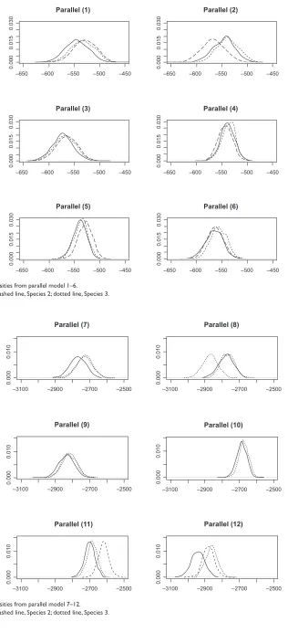
We collect LogPrs from 1000 Monte Carlo simulations. The distribution of these LogPrs are plotted in Figures 3, 4, 5 and 6. A Kolmogorov–Smirnov normality test gives p-value

(0.15) for all LogPr sets, which means that the difference

between the produced LogPrs and a normally distributed random variable is not significant. The normality assumption for LogPrs holds and the probability approximation based on log-normal distribution is reasonable. For such an assump-tion, a heuristic justification without rigorous theoretical proof is as follows: Given each randomly produced ancestor sequence, each nucleotide (event) LogPr on the non-reference sequences acts as an independently and identically distributed random variable, and the summation of these LogPrs follows

the central limit theorem for a large sample size (sequence length). By increasing the ancestor or root length from 100 to 500, we can see that the relationship between LogPr and the sequence length is approximately linear. Another observa-tion from Tables 2 and 3 is that different reference species sequences may lead to inconsistent sequence set probabilities due to different evolution durations and/or topological locations within the phylogenic structure. The phylogenic evolution model (the right panel of Figure 1) seems to show more inconsistency than the parallel evolution model (the left panel of Figure 1) does due to the dual missing sequences (the root and ancestor) instead of ancestor only in the paral-lel evolution model. A reference sequence which is closer to the root and/or ancestor is preferable since the imputed multiple roots and/or ancestors tend to be more informative due to shorter divergence. The CLUSTAL W multiple

align-ment12_{-induced probability is obtained by moving along the}

sequence set which holds nucleotides {ATCG} and possible

gaps (covalent bonds) and applying Rivas9_{model, where “one}

gap with two nucleotides” across three matched sequence sites stands for a deletion and “two gaps with one nucleotide” across three matched sequence sites stands for an insertion. For each simulated sequence set, the discrepancy between Monte Carlo integration (MCI) and single multiple alignment (MA) induced probabilities are clearly more significant than that among probabilities estimated from different reference species sequences.

CREB

promoters study

From the ABS database,13_{we extracted the promoter regions}

of transcription factor CREB for three mammals (human,

Table 1 Simulation configurations (parallel [PA] and phylogenic [PH] evolution models, α= 1.0)

No β t₀ t₁ t₂ t₃ q₀ L₀

(PA, Ph) (PA, Ph) (PA, Ph) (PA, Ph)

1 0.05 n/A, 0.05 0.10, 0.10 0.10, 0.05 0.10, 0.05 0.95 100

2 0.05 n/A, 0.05 0.10, 0.10 0.20, 0.15 0.10, 0.05 0.95 100

3 0.05 n/A, 0.10 0.20, 0.20 0.20, 0.10 0.20, 0.10 0.95 100

4 0.20 n/A, 0.15 0.30, 0.30 0.30, 0.15 0.30, 0.15 0.90 100

5 0.20 n/A, 0.15 0.30, 0.30 0.60, 0.45 0.30, 0.15 0.90 100

6 0.20 n/A, 0.01 0.05, 0.05 0.05, 0.04 0.05, 0.04 0.80 100

7 0.05 n/A, 0.05 0.10, 0.10 0.10, 0.05 0.10, 0.05 0.95 500

8 0.05 n/A, 0.05 0.10, 0.10 0.20, 0.15 0.10, 0.05 0.95 500

9 0.05 n/A, 0.10 0.20, 0.20 0.20, 0.10 0.20, 0.10 0.95 500

10 0.20 n/A, 0.15 0.30, 0.30 0.30, 0.15 0.30, 0.15 0.90 500

11 0.20 n/A, 0.15 0.30, 0.30 0.60, 0.45 0.30, 0.15 0.90 500

12 0.20 n/A, 0.01 0.05, 0.05 0.05, 0.04 0.05, 0.04 0.80 500

(7)

Parallel (1)

–650 –600 –550 –500 –450

0.000

0.015

0.030

Parallel (2)

–650 –600 –550 –500 –450

0.000

0.015

0.030

Parallel (3)

–650 –600 –550 –500 –450

0.000

0.015

0.030

Parallel (4)

–650 –600 –550 –500 –450

0.000

0.015

0.030

Parallel (5)

–650 –600 –550 –500 –450

0.000

0.015

0.030

Parallel (6)

–650 –600 –550 –500 –450

0.000

0.015

0.030

Figure 3 Log(probability) densities from parallel model 1–6.

Notes: solid line, species 1; dashed line, species 2; dotted line, species 3.

Figure 4 Log(probability) densities from parallel model 7–12.

0.010

0.000

–3100 –2900 –2700 –2500

Parallel (7)

0.010

0.000

–3100 –2900 –2700 –2500

Parallel (8)

0.010

0.00

0

–3100 –2900 –2700 –2500

Parallel (10)

0.010

0.00

0

–3100 –2900 –2700 –2500

Parallel (9)

0.01

0

0.00

0

–3100 –2900 –2700 –2500

Parallel (11)

0.01

0

0.00

0

–3100 –2900 –2700 –2500

Parallel (12)

(8)

Figure 5 Log(probability) densities from phylogenic model 1–6.

0.000

0.015

0.030

–700 –650 –600 –550 –500 –450 –400

Phylogenic (1)

0.000

0.015

0.030

–700 –650 –600 –550 –500 –450 –400

Phylogenic (2)

0.00

0

0.015

0.030

–700 –650 –600 –550 –500 –450 –400

Phylogenic (4)

0.00

0

0.015

0.030

–700 –650 –600 –550 –500 –450 –400

Phylogenic (3)

0.00

0

0.01

5

0.03

0

–700 –650 –600 –550 –500 –450 –400

Phylogenic (5)

0.00

0

0.01

5

0.03

0

–700 –650 –600 –550 –500 –450 –400

Phylogenic (6)

Figure 6 Log(probability) densities from phylogenic model 7–12.

0.000

0.010

–3400 –3200 –3000 –2800 –2600

Phylogenic (7)

0.000

0.010

–3400 –3200 –3000 –2800 –2600

Phylogenic (8)

0.000

0.010

–3400 –3200 –3000 –2800 –2600

Phylogenic (10)

0.000

0.010

–3400 –3200 –3000 –2800 –2600

Phylogenic (9)

0.000

0.010

–3400 –3200 –3000 –2800 –2600

Phylogenic (11)

0.000

0.010

–3400 –3200 –3000 –2800 –2600

Phylogenic (12)

(9)

mouse and rat). We used MEGA 4.1 package14_{to construct}

the phylogeny tree with corresponding divergence times under uniform transition rate 1 (see Figure 7). These are used for sampling the posterior ancestor and root.

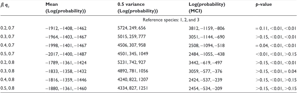
Since no current packages give us β and q₀ maximum

likelihood estimation for Rivas9_{model (Eq. (14)), we mainly}

investigate the sequence set probability sensitivity to β and

q₀ input by trying different values. We report the means

and variances as well as estimated Log(sequence set

prob-abilities) under two parameter settings for β and q₀ under

different reference species. We also report the p-values

from Kolmogorov–Smirnov normality test (Table 4). The normality test results are sensitive to parameter input and reference species selection, which may be due to the fact that conservation levels/transition probabilities are likely to be nonhomogeneous along the sequences. Two LogPr distributions under associated parameter inputs are plotted in Figure 8. As a verification, we apply multiple alignment to these three promoters and at each site we calculate the nucleotide identity proportion within the window (with size 23) starting from this site at the gene direction (Figure 9). The conservation levels show that evolutionary transition rates

Table 2 Computation results (parallel evolution models)

No Mean

(Log(probability))

0.5 variance (Log(probability))

Log(probability) (MCI)

Length (MA)

Log(probability) (MA)

Reference species: 1, 2, and 3

1 -544, -528, -533 267, 257, 263 -277, -270, -270 104 -1343 2 -545, -567, -538 229, 252, 231 -317, -315, -307 104 -1343 3 -572, -565, -568 197, 205, 212 -376, -361, -356 109 -1344 4 -538, -543, -536 92, 99, 87 -447, -444, -450 112 -1143 5 -539, -528, -537 88, 100, 91 -450, -429, -446 108 -1118 6 -565, -563, -556 152, 130, 119 -413, -432, -437 123 -1056 7 -2767, -2727, -2734 1135, 1130, 1121 -1632, -1597, -1613 536 -6825 8 -2775, -2868, -2766 1026, 970, 853 -1748, -1898, -1913 535 -6823 9 -2835, -2815, -2822 1008, 937, 853 -1827, -1879, -1969 533 -6801 10 -2684, -2683, -2673 434, 459, 412 -2249, -2225, -2261 533 -5786 11 -2700, -2620, -2685 455, 451, 429 -2245, -2170, -2257 538 -5678 12 -2940, -2878, -2860 763, 535, 580 -2177, -2342, -2280 630 -5413 Abbreviations: MCi, Monte Carlo integration; MA, multiple alignment.

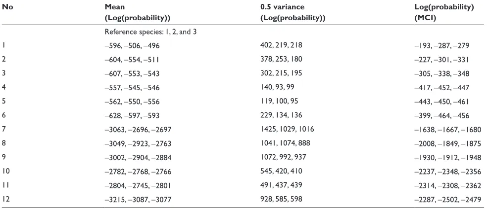
Table 3 Computation results (phylogenic evolution model)

No Mean

1 -596, -506, -496 402, 219, 218 -193, -287, -279

2 -604, -554, -511 378, 253, 180 -227, -301, -331

3 -607, -553, -543 302, 215, 195 -305, -338, -348

4 -557, -545, -546 140, 93, 99 -417, -452, -447

5 -562, -550, -556 119, 100, 95 -443, -450, -461

6 -628, -597, -593 229, 134, 136 -399, -464, -456

7 -3063, -2696, -2697 1425, 1029, 1016 -1638, -1667, -1680

8 -3049, -2923, -2763 1041, 1074, 888 -2008, -1849, -1875

9 -3002, -2904, -2884 1072, 992, 937 -1930, -1912, -1948

10 -2782, -2768, -2766 545, 420, 410 -2237, -2348, -2356

11 -2804, -2745, -2801 491, 437, 439 -2314, -2308, -2362

12 -3215, -3087, -3077 928, 585, 598 -2287, -2502, -2479

Abbreviation: MCi, Monte Carlo integration.

(10)

are approximately constant piece-wisely, thus the central limit theorem discussed for the simulated data study may still apply to these LogPrs on each promoter segment with quasi-constant conservation level under certain nucleotide

insertion-deletion parameter (β, q₀) values.

Discussion

We proposed and investigated some promising numerical algorithms for accurately estimating the probability of a set of orthologous sequences with equal length under certain assumptions. Our approach was to informatively shuffle the unknown ancestors and/or roots and to find the distribu-tional characteristics of simulated log-probabilities in order to reasonably approximate the true probability. The merit of our approach depends on how well the ancestor and/or root is imputed based on certain pentanomial distribution

proportions (p_-, p_A, p_T, p_C, p_G) in Eq. (16) using the evolution

model9_{and how reliably the pairwise Needleman-Wunsch}

alignment is applied to cross-species matching of nucleotides which are supposed to come from the same ancestor entry

{-, A, T, C or G}. The former depends on the divergence

duration from the ancestor/root to the reference sequence and the latter may depend on the species-specific adjustment of pairwise alignments based on phylogenic information.

When this piece of information is not immediately

avail-able, the algorithms by Yang,15_{Redelings and Suchard,}11

and MEGA package14_{are useful. Recently, Wong and}

col-leagues16_{demonstrated that various alignments may lead to}

quite inconsistent inference. Although distance estimation for multiple species from a common ancestor may lack some accuracy using only one sequence set (Figure 9), we used MEGA package for phylogenic structure information for real sequence set probability estimation. Note that we only use background sequences as examples to demonstrate our algorithms by assuming independent tetranomial dis-tribution among {ATCG} along sequences. For the set of

orthologous sequences involving many species (3), we

follow the evolutionary process (described by a phylogenic tree) to sample the internal nodes within the phylogenic tree conditional on one selected reference sequence (a terminal node on the phylogenic tree) and apply Monte Carlo integra-tion to these imputed internal nodes for obtaining LogPrs (we omit the details). As one referee points out, it may be unreliable to directly apply our algorithms to sequences with very irregular lengths, since the insertion–deletion events need to be identified by matching nucleotides across all involved species other than due to artificial sequence truncation. Thus a crude multiple alignment across such

0.300

0.208

0.045

0.092

Human

Mouse Rat

Figure 7 Phylogeny tree for orthologous CREB promoters.

Table 4 Computation results for CREB promoter sequence set (phylogenic evolution models)

β, q0 Mean

p-value

0.2, 0.7 -1912, -1408, -1462 5724, 249, 656 3812, -1159, -806 = 0.11, 0.01, 0.01 0.3, 0.7 -1964, -1403, -1467 5015, 259, 777 3051, -1144, -690 0.15, 0.01, 0.01 0.4, 0.7 -1998, -1401, -1467 4506, 307, 958 2508, -1094, -518 = 0.04, 0.01, 0.01 0.5, 0.7 -2017, -1400, -1487 4501, 345, 1049 2484, -1055, -438 0.01, 0.01, 0.15 0.2, 0.8 -1789, -1361, -1424 5231, 742, 927 3442, -619, -497 0.15, 0.01, 0.01 0.3, 0.8 -1833, -1358, -1432 4892, 781, 1056 3059, -577, -376 0.15, 0.01, = 0.04

0.4, 0.8 -1816, -1359, -1446 4240, 822, 1207 2424, -537, -239 0.15, 0.01, 0.15 0.5, 0.8 -1880, -1361, -1460 4334, 827, 1251 2454, -534, -209 0.15, 0.01, 0.15 Abbreviation: MCi, Monte Carlo integration.

(11)

Figure 8 Distribution of LogPrs (CREB promoters).

Reference = Human Reference = Mouse Reference = Rat

Log(probability) distribution

(

CREB

promoters, phylogenic model)

–2400 –2200 –2000 –1800 –1600 –1400 –1200

0.00

0

0.015

0.030

Beta = 0.2, q₀ = 0.8

Reference = Human Reference = Mouse Reference = Rat

Log(probability) distribution

(

CREB

promoters, phylogenic model)

–2400 –2200 –2000 –1800 –1600 –1400 –1200

0.000

0.015

0.030

Beta = 0.5, q₀ = 0.7

0 100 200 300 400 500

Location along upstream promoter region (from left to right)

0.0

0.2

0.4

0.6

0.8

1.0

Nucleotide identity proportion

Conservation level along CREB promoter region

Figure 9 nucleotide identity proportion along the upstream promoter regions for transcription factor CREB.

(12)

Advances and Applications in Bioinformatics and Chemistry

Publish your work in this journal

Submit your manuscript here: http://www.dovepress.com/advances-and-applications-in-bioinformatics-and-chemistry-journal Advances and Applications in Bioinformatics and Chemistry is an

international, peer-reviewed open-access journal that publishes articles in the following fields: Computational biomodelling; Bioinformatics; Computational genomics; Molecular modelling; Protein structure modelling and structural genomics; Systems Biology; Computational

Biochemistry; Computational Biophysics; Chemoinformatics and Drug Design; In silico ADME/Tox prediction. The manuscript management system is completely online and includes a very quick and fair peer-review system, which is all easy to use. Visit http://www.dovepress.com/ testimonials.php to read real quotes from published authors.

Dove

press

sequences may overly produce insertion and/or deletions. A rough solution may involve first applying multiple align-ment procedures to these sequences and then segalign-menting the aligned sequences into subsequences involving different numbers of species followed by segment-wise Monte Carlo integration. However, the internal edge-effects introduced by segmentation deserves further study. Lastly, we highlight that applying the proposed algorithms to real sequences is not so straightforward in view of heterogeneous conserva-tion patterns along the orthologous sequences, which poses as an important future research topic.

Acknowledgments

We thank Terence P Speed for his directions on evolution models when he visited Yale Center for Statistical Genomics and Proteomics (YCSGP) in May 2004. We are also grate-ful to Stéphane Robin and many anonymous referees for their constructive and insightful comments which greatly improved our work.

Disclosure

The authors report no conflicts of interest in this work.

References

1. Needleman SB, Wunsch CD. A general method applicable to the search for similarities in the amino acid sequence of two proteins. J Mol Biol. 1970;48:443–453.

2. Liu JS, Neuwald AF, Lawrence CE. Markovian structures in biological sequence alignment. J Am Stat Assoc. 1994;94:1–15.

3. Kellis M, Patterson N, Endrizzi M, Birren B, Lander ES. Sequencing and comparison of yeast species to identify genes and regulatory elements. Nature. 2003;423:241–254.

4. Moses AM, Chiang DY, Eisen MB. Phylogenetic motif detection by expectation-maximization on evolutionary mixtures. Pac Symp Biocomput. 2004;324–335.

5. Xie J, Li K-C, Bina M. A Bayesian insertion/deletion algorithm for distant protein motif searching via entropy filtering. J Am Stat Assoc. 2004;99(466):409–420.

6. Wei Z, Jensen ST. GAME: detecting cis-regulatory elements using a genetic algorithm. Bioinformatics. 2006;22:1577–1584.

7. Sinha S, He X. MORPH: Probabilistic alignment combined with hidden Markov models of cis-regulatory modules. PLoS Comput Biol. 2007;3(11):e216.

8. Jukes TH, Cantor CR. Evolution of protein molecules. In: Munro HN, editor. Mammalian Protein Metabolism. New York: Academic Press 1969; p. 21–132.

9. Rivas E. Evolutionary models for insertions and deletions in a proba-bilistic modeling framework. BMC Bioinformatics. 2005;6:63. 10. Lutzoni F, Wagner P, Reeb V, Zoller S. Integrating ambiguously aligned

regions of DNA sequences in phylogenetic analyses without violating positional homology. Syst Biol. 2000;49:628–651.

11. Redelings BD, Suchard MA. Joint Bayesian estimation of alignment and phylogeny. Syst Biol. 2005;54(3):401–418.

12. Higgins D, Thompson J, Gibson T, Thompson JD, Higgins DG, Gibson TJ. CLUSTAL W: improving the sensitivity of progressive multiple sequence alignment through sequence weighting, position-specific gap penalties and weight matrix choice. Nucleic Acids Res. 1994;22:4673–4680.

13. Blanco E, Farré D, Albà M, Messeguer X, Guigò R. ABS: a database of annotated regulatory binding sites from orthologous promoters. Nucleic Acids Res. 2006;34:D63–D67.

14. Tamura K, Dudley J, Nei M, Kumar S. MEGA4: Molecular evolutionary genetics analysis. Mol Biol Evol. 2007;24:1596–1599.

15. Yang Z. Maximum-likelihood estimation of phylogeny from DNA sequences when substitution rates differ over sites. Mol Biol Evol. 1993;10:1396–1401.

16. Wong KM, Suchard MA, Huelsenbeck JP. Alignment uncertainty and genomic analysis. Science. 2008;319:473–476.