Navigating Earthquake Physics with High-Resolution Array Back-Projection

(1)

Navigating Earthquake Physics with

High-Resolution Array Back-Projection

Thesis by

Lingsen Meng

In Partial Fulfillment of the Requirements for the Degree of

Doctor of Philosophy

CALIFORNIA INSTITUTE OF TECHNOLOGY Pasadena, California

2013

(2)

(3)

(4)

Shengji Wei, Dr. Risheng Chu , Dr. Fanchi Lin, and Dr. Wenzheng Yang for their advice and help both with questions in my research and life around Caltech. Carl and Lijun set the standard of suc-cessful Caltech graduates that I will aim to emulate. I also enjoyed socializing with Dongzhou, Xi Zhang, Da Yang, Dan Bower, Caitlin Murphy, Laura Alisic, Nina Lin, Yu Wang, Ting Chen, Zhongwen Zhan, Nneka Williams, Francisco Ortega, Xiangyan Tian, Yiran Ma, Dunzhu Li, and many other students, and I cherish their friendship. I am thankful to the helpful and friendly staff, Julia Zuckerman, Viola Carter, Dian Buchness, and Donna Mireles, who has been heroes behind the success of every Seismo Lab researcher.

I thank Anthony Sladen, Herbert Redon, Wenbo Wu, Sidao Ni, Morgan Page, Ken Hudnut, and Zach Duputel who has been very dedicated and responsive during our collaborations. I also thank my colleagues working on earthquake source imaging, Miyaki Ishii, Alex Hukto, Huajian Yao, Pe-ter Shearer, Thorne Lay, and Keith Koper who had very inPe-teresting discussions with me at various conferences.

(5)

(6)

(7)

(8)

(9)

(10)

(11)

(12)

D.3 Comparison of the unwrapped InSAR images for the kinematic slip model ... 147

D.4 Comparison of the wrapped InSAR images for the kinematic slip model ... 148

D.5 Predicted surface deformation ... 150

D.6 Head-on view of the slip distribution for our preferred kinematic model ... 151

D.7 Surface projection of the preferred static slip model (InSAR+GPS) ... 152

D.8 Head-on view of the slip distribution for our preferred static slip model ... 153

D.9 Comparison of the unwrapped InSAR images for the static slip model ... 154

D.10 Comparison of the wrapped InSAR images for the static slip model ... 156

(13)

LIST OF TABLES

Number Page

4.1 Parameters of the 4 dynamic models shown in Figure 4.3 ... 49

A.1 1D velocity model for Japan ... 116

C.1 Parameters of the 4 dynamic models shown in Figure C.2 ... 143

(14)

(15)

(16)

(17)

(18)

(19)

(20)

(21)

(22)

Figure 1.2. Sketch of beamforming back-projection (figure adopted from Alex Hutko’s

2009 AGU talk). The black dots in the center of the rectangular grids indicate the location

of testing sources. The true source location (red star) is connected to the receivers (black

triangles) through ray theory. The black curves above the receivers denote the recorded

seismograms. In principle, the moveout of true source locations (red lines) brings the

(23)

(24)

(25)

(26)

(27)

(28)

(29)

(30)

(31)

(32)

(33)

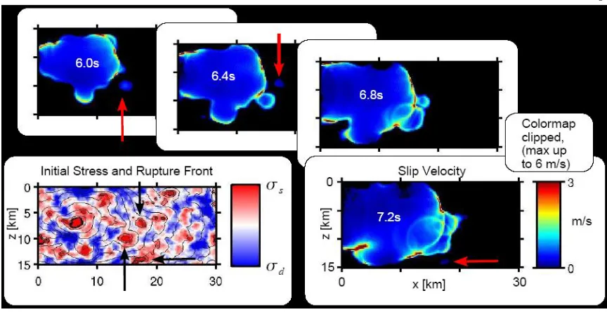
pershear phenomena, since the back-projection tends to image apparent secondary sources with small power connecting true sources (Figure A.7). This artifact is unlikely for the Tohoku-Oki earthquake, since the power is almost uniform during the supershear stage. However, the very fast front propagates mainly along strike and existing theoretical models do not allow supershear rup-tures in mode III. Along-strike supershear rupture in subduction earthquakes requires a significant along-strike slip component or yet unexplored mode coupling processes that efficiently break the mode III symmetries. While the second strong phase observed in the strong motion data can be as-sociated to the HF radiation found in dynamic rupture models during the transition to supershear speeds, this is not a unique interpretation. Further signatures of supershear propagation might be found in the local strong motion data if there is significant Mach cone radiation towards the land. Ocean bottom pressure gauges that recorded HF acoustic signals, especially stations TM1 and TM2, could also provide precious insight into this question.

(34)

(35)

(36)

(37)

(38)

(39)

(40)

(41)

(42)

(43)

(44)

(45)

(46)

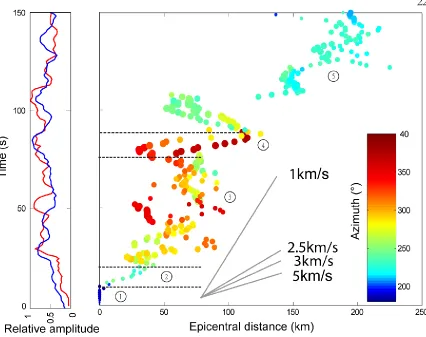
Figure 3.2. Spatiotemporal details of the rupture process. Left: timing and position of the high frequency radiators relative to the hypocenter. The position is reported in alternation along the axes labeled X (red) and Y (blue) in Fig.3.1-inset. Circles and squares are the results of Europe and Japan arrays, respectively. Filled and open symbols indicate principal and secondary high-frequency radiators, respectively. Inset: shear strength (τ) vs. normal stress (σ) diagram of a non-linear strength envelope with small apparent friction coefficient µ (almost pressure-insensitive material) and large cohesion C, resulting in almost orthogonal failure planes (Ө ~ 90°). Right: dynamic Coulomb stress changes induced near the tip of a right-lateral crack propagating at steady rupture speed, resolved onto orthogonal left-lateral faults in the compressional quadrant as a function of the ratio between rupture speed and shear-wave speed, [Poliakov et al. 2002]. The symbols denote dynamic changes of normal stress ( , negative compressive, blue dashed

line), shear stress ( , positive left-lateral, red dashed line) and Coulomb stress (

, color solid curves, assuming various apparent friction coefficients indicated in the leg-end). Stresses are normalized based on the Mode II stress intensity factor ( ) and the distance to

(47)

(48)

(49)

(50)

(51)

(52)

(53)

(54)

(55)

(56)

(57)

(58)

:

(59)

(60)

(61)

Figure 4.4. Maximum friction coefficient (µ) that allows compressive branching (positive dynamic Coulomb stress change near the rupture tip), as a function of rupture speed (Vr) and for three values of the Skempton coefficient B (see legend). The curves correspond to branching on an orthogonal fault, and the color bands encompass the range of fault orientations within the uncertainty inferred from the back-projection results (Figure 1). This analysis is based on analytical solutions for the dynamic stresses near a propagating rupture front (Poliakov et al. 2002). The numbers in circles indicate the parameters settings of the dynamic rupture models (with B = 0) shown in Figure 4.3, which confirm these analytical arguments.

(62)

Model index

µ

s

µ

d

C

σ

0

τ

0

Vr/Vs

dτ

Dc’

1

0

38 MPa

250 MPa

38 MPa

0.54

13 MPa

2.2e-3

2

0.2 0.1 0

250 MPa

38 MPa

0.54

13 MPa

2.2e-3

3

0.2 0.1 0

250 MPa

38 MPa

0.89

13 MPa

6e-4

4

0.6 0.4 0

250 MPa

115 MPa

0.54

15 MPa

1.5e-3

(63)

C h a p t e r 5

HIGH-RESOLUTION BACK-PROJECTION AT REGIONAL DISTANCE:

APPLICATION TO THE HAITI M7.0 EARTHQUAKE AND COMPARISONS

WITH FINITE SOURCE STUDIES

Originally published in L. Meng, J.-P. Ampuero, A. Sladen and H. Rendon (2012), High-resolution back-projection at regional distance: Application to the Haiti M7.0 earthquake and comparisons with finite source studies. J. Geophys. Res., 117, B04313.

Note: the supplementary materials are included in Appendix D.

5.1. Abstract

(64)

(65)

(66)

(67)

(68)

(69)

(70)

(71)

(72)

(73)

(74)

(75)

(76)

(77)

(78)

(79)

(80)

(81)

(82)

(83)

(84)

(85)

(86)

(87)

(88)

(89)

(90)

(91)

(92)

(93)

(94)

(95)

(96)

(97)

(98)

(99)

(100)

(101)

(102)

(103)

(104)

(105)

(106)

(107)

(108)

(109)

(110)

(111)

(112)

(113)

(114)

(115)

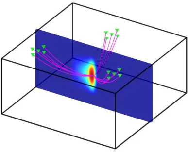
Figure 6.1. The “swimming” artifact of a 1D array in a 2D Earth.

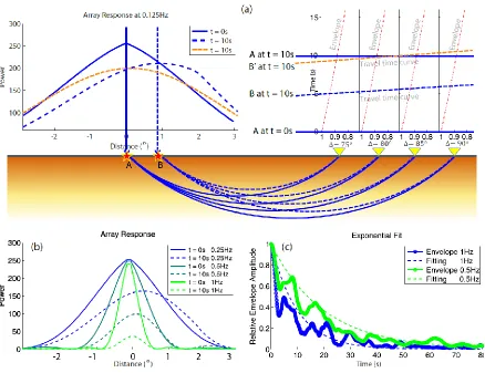
(a) “Swimming” effect at lower frequency (0.125 Hz) with respect to a teleseismic (75°-90°) linear array of 16 stations (1° spacing).

Upper left figure shows the artifact: at t = 10 s, maximum array response drifted from true location A (0°, as solid-edged star) to apparent location B (0.9°, dash-edged star), a difference of about 100 km.

(116)

(117)

(118)

(119)

(120)

(121)

reliable at periods shorter than 4 s. In lower frequencies, the spatial bias is notable but less se-vere than that of beamforming.

(122)

(123)

(124)

(125)

(126)

(127)

(128)

(129)

(130)

A.7. Analysis of Strong Motion Data

We examine velocity envelopes of strong motion data recorded along the northeastern Honshu coastline in order to identify prominent phases observed at teleseismic distances. We band pass fil-ter the data, integrate, square and sum traces of horizontal components. The resulting velocity enve-lopes are averaged using a sliding median filter whose length is equal to five times the lower bound of the band pass filter. Fig. A.10a and Fig. A.10b show scaled smoothed velocity envelopes for 0.5-1 Hz and 2.5-5 Hz frequency bands, respectively. We find that the prominent high-frequency bursts from locations that ruptured 33, 85, and 140 seconds after the mainshock are well resolved for fre-quencies as low as 0.5Hz. This observation is consistent with our results for the 5-10 Hz frequency band presented in the main text.

A.8. Velocity Model

In the analysis of the ground motion data recorded by the K-net and KiK-net seismic networks we use the following 1D model derived from [Takahashi et al. 2004] :

Table A.1. 1D velocity model in Japan.

Depth (km)

S-wave velocity (km/s)

0

3.46

16

3.87

(131)

A.9. Data Sources

We downloaded the data from the following sources: USArray: http://www.usarray.org/

European seismic network: http://www.orfeus-eu.org/ K-net: http://www.k-net.bosai.go.jp/

(132)

(133)

(134)

(135)

(136)

(137)

(138)

(139)

(140)

(141)

(142)

(143)

(144)

(145)

(bore-correspond to an assumed rupture speed of 2.5 km/s. The MUSIC back-projection technique recovers the location and timing of the scenario sources very well. The uncertainty of the peak loca-tions is less than 20 km, which is reasonably good considering the coda and interference between sub-sources. These synthetic tests indicate that the jump between faults C and D is resolvable by the Hi-Net array.

B.3. Multiple Point Source Analysis

(146)

(147)

(148)

(149)

(150)

(151)

(152)

(153)

(154)

Movie B.1: The movie shows the raw results of back-projection source imaging based on teleseismic data from European networks. Warm colors indicate the positions of the high frequency (0.5 to 1 Hz) radiation back-projected onto the source region based on IASP91 travel times [Snoke 2009]. The sliding window is 10 s long and the origin time is 08:38:37, 04-12-12 (UTC). The beginning of the sliding window is set to be 5 s before the initial P-wave arrival. Colors indicate the amplitude of the MUSIC pseudospectrum on a logarithmic scale (dB) after subtracting the background level and rescaling the maximum to the linear beamforming power in each frame separately. The white star is the mainshock epicenter and the green circles are the epicenters of the first day of aftershocks from the NEIC catalog. Time relative to hypocentral arrival time is shown on top. The trench and coastlines are shown by white curves.

(155)

A p p e n d i x C

(156)

(157)

(158)

(159)

in-A p p e n d i x D

(160)

(161)

(162)

Figure D.3. Comparison of the unwrapped InSAR images for the kinematic slip model.

(163)

(164)

(165)

(166)

(167)

(168)

(169)

(170)

(171)

(172)

(173)

(174)

(175)

(176)

(177)

(178)

(179)

(180)

(181)

(182)

(183)

(184)

(185)

rup-Zhang, H., Z. Ge and L. Ding (2011), Three sub-events composing the 2011 off the Pacific coast of Tohoku Earthquake (Mw 9.0) inferred from rupture imaging by back-projecting teleseis-mic P waves, Earth Planets Space, Vol. 63 (No. 7), pp. 595-598.

Zhu, L. P., and D. V. Helmberger (1996), Advancement in source estimation techniques using broadband regional seismograms, Bull. Seismol. Soc. Am., 86(5), 1634–1641.