The Low-Frequency Frontier: Cosmology with Future 21cm Experiments

(1)

Cosmology with Future 21cm Experiments

Thesis by

Abhilash Mishra

In Partial Fulfillment of the Requirements for the degree of

Doctor of Philosophy

CALIFORNIA INSTITUTE OF TECHNOLOGY Pasadena, California

2018

(2)

Abhilash Mishra

ORCID: 0000-0002-4424-4096

(3)

(4)

"[The Emperor Kublai Khan] said: "It is all useless, if the last landing place can only be the infernal city, and it is there that, in ever-narrowing circles, the current is drawing us."

To which Marco Polo replied: "The inferno of the living is not something that will be; if there is one, it is what is already here, the inferno where we live every day, that we form by being together. There are two ways to escape suffering it. The first is easy for many: accept the inferno and become such a part of it that you can no longer see it. The second is risky and demands constant vigilance and apprehension; seek and learn to recognize who and what, in the midst of the inferno, are not inferno, then make them endure, give them space."

-Italo Calvino, Invisible Cities

"It might seem limited to impose our human perception to try to deduce the grandest cosmic code. But we are the product of the universe and I think it can be argued that the entire cosmic code is imprinted in us. Just as our genes carry the memory of our biological ancestors, our logic carries the memory of our cosmological ancestry. We are not just imposing human-centric notions on a cosmos independent of us. We are progeny of the cosmos and our ability to understand it is an inheritance."

(5)

ACKNOWLEDGEMENTS

The opportunity to participate in the scientific enterprise is a great privilege and I would not have embarked on this journey without the early encouragement and support from my teachers and mentors. Rinku Sarangi got me hooked on science in high school; she remains the best teacher I’ve met. Swadhin Pattanayak introduced me to the joys of research; his love for science and commitment to social justice continues to inspire me. Raka Dabhade, Ajit Kembhavi, Rajaram Nityananda, T Padmanabhan, and Subir Sarkar converted me to astrophysics; I’m grateful to them for helping me get here.

This thesis would not have been possible without the support from my advisor Chris Hirata. Chris’ brilliance is matched only by his humility and generosity. He gave me the space to make my own mistakes, nudged me towards working on important problems, and was incredibly patient with me. His ability to bring forth the essential physics of a problem and his attention to detail is awe inspiring. I’m immensely grateful to him for supporting me through these years. My co-advisor Olivier Doré was kind to adopt me into his group. He has fostered a lively and diverse group of young cosmologists at Caltech and JPL and I learned a lot of astrophysics through the weekly journal clubs and group meetings he organized. His insight, advice, and sense of humor has kept me going during tough times and I thank him for his support. I’d also like to thank other members of my thesis committee: Lynne Hillenbrand, Shri Kulkarni, and Gregg Hallinan for their time and advice.

My work during grad school would not have been possible without my collabora-tors Michael Eastwood, Roland de Putter, Barnaby Rowe, Eric Linder, and Vera Gluscevic. I thank them for their dedication and for sharing their time and expertise with me. The Cahill cosmology and theoretical astrophysics community played an important role in teaching me about interesting astrophysical problems during the formative years of grad school. I thank Samaya Nissanke, Francis-Yan Cyr-Racine, Duncan Hanson, Alvise Raccanelli, Phil Bull, Jérôme Gleyzes, Andrew Benson, and Heidi Wu for sharing their ideas and insights.

(6)

always cherish the times we spent together. I thank Aaron Zimmerman for being an amazing friend and mentor. Aaron is a role model to me in many ways and I learned a lot about astrophysics and life over coffee at Red Door. My academic siblings, Antonija Oklopčić, Tejaswi Venumadhav, Elisabeth Krause, and Denise Schmitz always looked out for me and were generous with their time and support. Working on homework sets during the first two years of grad school was a lot of fun because of John Wendell and Kristen Boydstun. I thank them for converting me to Python and educating me about American pop culture. Alicia Lanz and Allison Strom were thoughtful, inspiring leaders in the Caltech student community during a particularly difficult time for the Institute. I’m very lucky to call them friends. My fellow grad students in Cahill, Mislav Baloković, Trevor David, Ben Montet, Matt Orr, Gina Duggan, Donal O’Sullivan, Jacob Jencson, Melodie Kao, Sebastian Pineda, Sherwood Andrew Richers, Elena Murchikova, Jackie Villadsen, Marin Anderson, Becky Jensen-Clem, and Bhawna Motwani made Cahill a warm and welcoming place to work. “The Elders”: Mansi Kasliwal, Varun Bhalerao, Gwen Rudie, Drew Newmann, Laura Perez, and Matthew Stevenson worked really hard to build a supportive, tight-knit grad student body in astrophysics, and shaped Cahill to be a warm, collegial place for doing astrophysics. Thanks also to Anu Mahabal, Patrick Shopbell, Joy Painter, JoAnn Boyd, Gita Patel, Shirley Hampton, and everyone at the Caltech Dean’s office for their helpfulness and generosity.

Grad school can be rather isolating but I’m thankful for the friends around the world who cheered me on along the way. Many thanks to Chris Sheppard and Rakesh Sharma for reminding me that there is a life outside of work. Io Kleiser and Matt Gethers for the laughter and the countless expeditions to WeHo. Mike Bottom and Heather Duckworth for the sparkling conversations, the bad movie nights and cake. Judith and Steve Marosvolgyi for their kindness. Sara Hubbard, Lee Thiesen, George Olive, and Ziyaad Bhorat for their friendship and for introducing me to the many delights of Los Angeles. Krishna Shankar and Ashish Goel for being the best house-mates one could ask for.

(7)

works, no matter where they live. I’m very excited to continue this work during the next stage of my career.

My friends Indra and Pinkesh, have taught me so much over the years. Their friendship means the world to me and nothing I write here can do justice to what I owe them.

One of the most difficult events over the past few years was the passing of my friend Ishita Maity. Her passing left a void that will never be filled. I miss her.

(8)

ABSTRACT

This thesis presents theoretical and observational investigations in two areas of cosmology: the detection of inflationary gravitational waves using the circular polarization of the redshifted 21cm line from neutral hydrogen during the Dark Ages, and the study of galactic foregrounds at low-frequencies using the Owens Valley Radio Observatory Long Wavelength Array (OVRO LWA).

In the theoretical part of this thesis, we propose a new method to measure the tensor-to-scalar ratior using the circular polarization of the 21 cm radiation from the Dark Ages. In Chapter II we discuss the basic principles of inflationary physics, which is now accepted as a standard paradigm for the generation of perturbations in the early universe. Along with density (scalar) perturbations, inflation also produces gravitational wave (tensor) modes. In Chapter IV we outline a novel, albeit futuristic method to detect inflationary gravitational waves. Our method relies on the splitting of theF =1 hyperfine level of neutral hydrogen due to the quadrupole moment of the CMB during the Dark Ages. We show that unlike the Zeeman effect, whereMF = ±1

have opposite energy shifts, the CMB quadrupole shifts MF = ±1 together relative

toMF =0. This splitting leads to a small circular polarization of the emitted 21cm

photon, which is in principle observable. Further, we forecast the sensitivity of future radio experiments to measure the CMB quadrupole during the era of first cosmic light (z ∼20). The tomographic measurement of 21 cm circular polarization allows us to construct a 3D remote quadrupole field. Measuring the B-mode component of this remote quadrupole field can be used to put bounds on the tensor-to-scalar ratio r. We make Fisher forecasts for a future Fast Fourier Transform Telescope (FFTT), consisting of an array of dipole antennas in a compact grid configuration, as a function of array size and observation time. The forecasts are dependent on the evolution of the Lyman-α flux in the pre-reionization era, that remains observationally unconstrained. Finally, we calculate the typical order of magnitudes for circular polarization foregrounds and comment on their mitigation strategies. We conclude that detection of primordial gravitational waves with 21 cm observations is in principle possible, so long as the primordial magnetic field amplitude is small, but would require a very futuristic experiment with corresponding advances in calibration and foreground suppression techniques.

(9)

(10)

PUBLISHED CONTENT AND CONTRIBUTIONS

Mishra, A., & Hirata, C. M., 2017, ArXiv e-prints, arXiv:1707.03514,

(11)

LIST OF FIGURES

Number Page

1.1 The cosmic microwave background map after removal of galactic and extragalactic foregrounds from the Planck mission gives us a snapshot of a nearly homogeneous universe around 380,000 years after the big bang. . . 3 1.2 Different cosmological probes and the length scales they probe adapted

from Tegmark & Zaldarriaga 2002: The figure shows power spec-trum of density fluctuations in the Universe as predicted by theΛCDM model (red line) and the various probes used to measure the power spectrum at different length scales. This figure is based on data available in 2002 and cosmological LSS probes have advanced sig-nificantly since then. However, the essential mapping of probes to scales is the same. . . 4 2.1 Conformal diagram for standard FRW cosmology. In standard

cos-mology there are∼ 105causally disconnected patches (figure adopted from Baumann 2009). . . 10 2.2 Inflation extends conformal time to negative values. The end of

inflation is atτ=0. As we can see in the figure, causally disconnected patches atτ=0 were in causal contact before inflation (figure adopted from Baumann 2009). . . 11 2.3 Inflation postulates that the energy density of the universe is

dom-inated by the vacuum energy associated with the displacement of a scalar field (the inflaton). The inflaton potential is unknown and needs to be constrained by observations. Here, shown for illustration are two toy models for the inflaton potential from ((figure adopted from Kamionkowski & Kovetz 2016)). . . 13 2.4 All scales that are relevant to cosmological observations today were

(14)

2.5 Current constraints on the scalar spectral indexnsand tensor-to-scalar

ratior, for a variety of slow-roll inflationary models. Figure adopted from Planck Collaboration et al. 2016. . . 24 2.6 The top panel shows a polarization pattern composed only of E

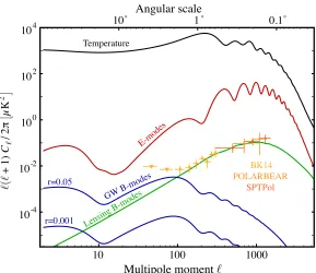
modes. The polarization pattern is tangential around hot spots and radial around cold spots. The bottom panel shows a polarization pattern composed only of B modes. The polarization pattern sur-rounding hot and cold spots of the Bmode show a swirling pattern. Note that the E-mode is parity invariant while the B-mode is not. Figure adopted from Kamionkowski & Kovetz 2016. . . 25 2.7 Theoretical predictions for the temperature (black), E-mode (red),

and tensor B-mode (blue) power spectra. Also shown are expected values lensing B-modes (green). Current measurements of the B-mode for BICEP2/Keck Array (yellow), POLARBEAR (orange), and SPTPol (dark orange). Figure adopted from Abazajian et al. 2016. . . 26 3.1 21 cm observations can potentially map the largest volumes of the

observable universe, while the CMB can probe a 2D surface at z ∼ 1100. and LSS surveys can map small volumes of the local universe. Note that more than half of the comoving volume of the universe lies atz > 20. Figure adopted from Tegmark & Zaldarriaga 2009. . . 31 3.2 The transitions relevant for the Wouthuysen-Field effect. Solid line

transitions contribute to spin flips. Transitions denoted by dashed lines are allowed but do not contribute to spin flips. Figure adopted from Pritchard & Loeb 2012. . . 33 3.3 The evolution of the 21 cm global signal depends on different

phys-ical processes at different epochs. The evolution of the brightness temperatureTb leads to the 21cm signal appear either in absorption

or in emission against the CMB. The top panel shows a slice through a simulation showing the evolution ofTb and the heating due to the

(15)

3.4 The evolution of the 21 cm power spectrum as a function of the ionized fraction is expected to reveal the astrophysical processes that drove reionization and the nature of the first stars and galaxies. The right side of the y-axis shows neutral fraction of the universe. As the universe goes from almost neutral (yellow) to ionized (gray), the overall amplitude of the power spectrum decreases. Moreover, as reionization proceeds the high-k power decreases since reionization bubbles start forming at small scales and then grow to larger scales. . 36 3.5 The evolution of the universe from the CMB (extreme left) to the

current day (extreme right). After the CMB the universe goes through the Dark Ages when it is largely neutral. As the first stars and galaxies light up, the universe gets reionized. Reionization is inhomogeneous and fills the the universe with merging bubbles of ionized hydrogen. Image credit: HERA/Avi Loeb/SciAm . . . 38 3.6 Schematic of a two antenna interferometer. . . 41 4.1 Energy Level Splitting . . . 54 4.2 Tomographic measurements by Fast Fourier Transform Telescopes

(FFTTs) would allow us to measure the remote quadrupole of the CMBa2m(z)(m =1,2) in volume pixels ("voxels") of volumeVcin narrow slice of redshift space. Creating a map of remote quadrupole moments across many voxels allows us to construct a spin-weightm field, which can be decomposed into E andBmodes. Measurement of theB-modes of this field allows us to put bounds on the tensor-to-scalar ratior. . . 58 4.3 Inputs used for the sensitivity calculation, computed for standard

cosmology using the 21CMFAST code. The plot shows the fiducial models for spin, kinetic, and CMB temperatures. . . 62 4.4 Inputs used for the sensitivity calculation, computed for standard

cosmology using the 21CMFAST code. The plot shows the fiducial models for quantities that parametrize the rate of depolarization of the ground state by optical pumping and atomic collisions as discussed in the text and in Gluscevic et al. 2017 . . . 63 4.5 Temperature, circular polarization, and noise power spectra relevant

(16)

4.6 Elements of the Fisher matrixw1as a function of redshiftz, computed for a model of reionization described in the text. For our fiducial model, both w1and w2 peak at z = 19.5, i.e. the redshift where the Lyman-alpha coupling becomes efficient ( ˜xα ∼1). . . 65

4.7 Elements of the Fisher matrixw2as a function of redshiftz, computed for a model of reionization described in the text. For our fiducial model, both w1and w2 peak at z = 19.5, i.e. the redshift where the Lyman-alpha coupling becomes efficient ( ˜xα ∼1). . . 66 4.8 Forecasts for σr for different FFTT telescope configurations. The

parameters used to make these forecasts are described in Fig. 4.4 & 4.3 and in Section 4.4. For the given Lyman-α flux model the values of weights w1 and w2 peak around z ∼ 19.5 as shown in Fig. 4.7. For our forecasts we consider a shell with zmin = 18 and

zmax = 23. Note that the live observation time quoted here will be

shorter than the wall-clock time of the survey. . . 72 4.9 Order of magnitude of expected foregrounds for the circular

polar-ization signal from Galactic synchrotron (purple line) and due to Faraday rotation through the ISM (orange line) compared against the noise power spectra expected for for three different configurations of FFTTs. . . 77 4.10 Order of magnitude of expected foregrounds for the circular

polar-ization signal from unresolved point sources (blue, green, and purple line)and Faraday rotation due to the ionosphere (orange line) com-pared against the noise power spectra expected for three different configurations of FFTTs. . . 79 5.1 Map of the antenna layout for OVRO LWA. Black circles correspond

to the 251 core antennas. The black triangles correspond to the 32 expansion antennas that extend the maximum baseline of the array. The 5 crosses are antennas equipped with noise-switched front ends for calibrated total power measurements. This figure was provided courtesy of Michael Eastwood and to be published in Eastwood et. al. (in prep) . . . 93 5.2 3-color all-sky map generated with m-mode analysis imaging

(17)

5.4 Cross-spectra between LWA map and Dust map with power injected in thel = 250−300 band . . . 103 5.5 Recovered auto-power spectrum of the dust map with power injected

in thel = 250−300 band . . . 104 5.6 Dust map correlations with the six LWA maps for the northern

sky-cut. The correlations are normalized with the auto-spectra as de-scribed in the text . . . 105 5.7 Hαmap correlations with the five LWA maps for the northern sky-cut.

The correlations are normalized with the auto-spectra as described in the text . . . 106 5.8 HI map correlations with the five LWA maps for the northern sky-cut.

The correlations are normalized with the auto-spectra as described in the text . . . 107 5.9 Upper limits on the dust emissivity at low-frequencies in terms of

τ100µm, the optical depth at 100µm. . . 109 5.10 Upper limits on the electron temperature as a function of scale from

(18)

LIST OF TABLES

Number Page

5.1 Summary of LWA maps used for cross-correlations . . . 104 5.2 Summary statistics fort-tests on the LWA×Dust cross-correlation to

check for zero correlation. The t-statistic is calculated for each ` bin under a null hypothesis that there is zero cross-correlation in the given ` bin, with 7 d.o.f. (since there are 8 jackknife regions). First row for a given ` band reports the t-statistic and the corresponding p-value is given in the second row for a given` band. . . 113 5.3 Summary statistics for t-tests on the LWA×Hα cross-correlation to

check for zero correlation. The t-statistic is calculated for each ` bin under a null hypothesis that there is zero cross-correlation in the given ` bin, with 7 d.o.f. (since there are 8 jackknife regions). First row for a given ` band reports the t-statistic and the corresponding p-value is given in the second row for a given` band. . . 114 5.4 Summary statistics for t-tests on the LWA×HI cross-correlation to

(19)

C h a p t e r 1

INTRODUCTION

“For the Ancient Greeks, the future was something that came upon them from behind their backs, with the past receding away before their eyes. When you think about it, that’s a more accurate metaphor than our present one. Who really can face the future? All you can do is project from the past, even when the past shows that such projections are often wrong. And who really can forget the past? What else is there to know?"

-Robert M. Pirsig, Zen and the Art of Motorcycle Maintenance

One of the most remarkable consequences of the theory of relativity is that our ability to look further into space allows us to peer back into our past. Over the last century, breathtaking theoretical and technological innovations have allowed us to probe large volumes of the universe, allowing us to reconstruct our cosmic history, from the Big Bang to the present day. Cosmology today is no longer an esoteric philosophical exercise; instead it is a rigorous empirical science.

An avalanche of data from the cosmic microwave background (CMB), galaxy sur-veys, gravitational lensing, supernova studies, cluster counts and chemical abun-dance studies have led to the construction of a "concorabun-dance" model of modern cosmology, with tightly constrained parameters. The broad consensus about the history of the universe is as follows: the universe began through an exponentially expanding phase called inflation, which seeded the initial perturbations in density. These density perturbations then grew via gravitational collapse to form stars and galaxies and the complex cosmic web we see today.

(20)

electromagnetic or strong interactions with baryonic matter, and likely don’t have any self-interaction). Together these compose the standard ΛCDM model of the universe.

While parameters of the concordance model of the universe are accurately measured, the physical underpinnings of these parameters remain far from clear. The biggest questions that remain unanswered are: what is dark matter? What is the nature of dark energy? How did the universe evolve from a smooth initial state to the complex structures we see around us? And finally, what is the physics of the process that generates perturbations in the early universe? The work presented in this thesis presents some new avenues to approach these questions. The first part of this thesis presents a novel way to test inflation using circular polarization of the 21cm line emitted by neutral hydrogen at high redshifts. The second part of the thesis investigates some observational challenges in probing the universe using 21cm radiation.

The rest of the chapter is organized as follows: in Sec. 1.1 we provide a whirlwind overview of different observational probes of the universe, in Sec. 1.3 we provide an overview of this thesis.

1.1 Measuring the Universe

The standard cosmological model is essentially parameterized by two functions: the cosmic expansion history a(t) and the cosmic clustering history, in terms of the power spectrum at different redshifts P(k,z). The cosmic expansion history is determined by the zeroth order Friedmann equation and depends on the energy budget of the universe as well as the equation of state of dark energy. The power spectrumP(k,z)can be factored as a product of theprimordialpower spectrum that depends on the physics of the early universe and a transfer function that characterizes the physics of late stage evolution.

There are several observational probes of P(k,z)using the fluctuations inside our observable horizon. The most widely-known is the Cosmic Microwave Background (CMB), which is the relic radiation from when the universe was around 400,000 years old. The density fluctuations in the CMB have been measured with exquisite precision by a number of experiments, most recently by the Planck satellite. Fig. 1.1 shows the map of the CMB after removal of galactic and extragalactic foregrounds.

(21)

Figure 1.1: The cosmic microwave background map after removal of galactic and extragalactic foregrounds from the Planck mission gives us a snapshot of a nearly homogeneous universe around 380,000 years after the big bang.

fluctuations in the universe at much smaller scales and at later stages. As such their interpretation has to deal with complicated non-linear effects as well as more messy astrophysics during the late stages of the universe. Fig. 1.2 from Tegmark & Zaldarriaga 2002 shows the different probes that measure the matter power spectrum at various scales. As evident from the figure, the CMB probes the largest scale fluctuations while Large Scale Structure (LSS) probes smaller and intermediate length scales.

1.2 The Low Frequency Frontier: Mapping the Universe with the21cm Line

(22)

Figure 1.2: Different cosmological probes and the length scales they probe adapted from Tegmark & Zaldarriaga 2002: The figure shows power spectrum of density fluctuations in the Universe as predicted by the ΛCDM model (red line) and the various probes used to measure the power spectrum at different length scales. This figure is based on data available in 2002 and cosmological LSS probes have advanced significantly since then. However, the essential mapping of probes to scales is the same.

today.

This thesis deals with theoretical and observational aspects of one of the frontiers of modern observational cosmology: the use of 21cm radiation from the hyperfine splitting of neutral hydrogen to probe the universe during the first billion years, from the so called Dark Ages to the late stage reionized universe. Current and upcoming 21cm experiments are poised to revolutionize cosmology by enabling a detailed understanding of astrophysics: when did the first stars form? When did reionization begin? What reionized the universe? 21cm experiments will also revolutionize cosmology and fundamental physics by allowing for the measurement of the largest accessible volume inside the horizon.

(23)

on reionization come from the absorption of the Lyman-α line in the spectra of high-redshift quasars. The optical depth to neutral hydrogen for Lyman-α pho-tons is extremely high, implying that even a small fraction of neutral hydrogen in the universe saturates the absorption signature. This leads to the Gunn-Peterson trough Gunn & Peterson 1965, which can help constrain the redshift when the uni-verse is almost entirely ionized. Observations indicate that this redshift is around z∼ 6. Large scale fluctuations in the polarization of the CMB also helps constrain the stage when the reionization was partially complete. Recent Planck data Planck Collaboration et al. 2016 indicates that the average redshift at which reionization occurs is is likely betweenz =7.8 and 8.8. The data also indicates that the Universe was ionized at less than the 10% level at redshifts abovez∼ 10 ruling out models of early reionization. Other constraints on reionization come from Lyman-αdamping wings of high redshift Gamma-Ray Bursts (Miralda-Escudé 1998; Barkana & Loeb 2004) and from the detection of high-redshift galaxies (Robertson et al. 2010).

While we have a broad-brush picture of the process of reionization, the details of the process are rather poorly understood. When did the first stars form and what was their composition? How did the first X-ray sources affect the evolution of the IGM? What was the role of blackholes, both supermassive as well as stellar mass? How did the Lyman-αbackground evolve just prior to reionization?

Astronomy, however, is still fundamentally a discovery driven science. As we shall see in subsequent chapters, the real promise of 21cm experiments lies in their ability to make 3D maps of the universe at scales that are unprecedented. This cosmic cartography will enable us to not just measure known cosmological parameters with great accuracy, it will very likely provide new surprises. The volumes that these experiments will open up will enable quite literally the largest physics laboratories in the universe. Beyond measuring cosmological parameters, this laboratory can potentially be used to answer fundamental physical questions such as constraining the strength of primordial magnetic fields, detect annihilating dark matter, or constraining models of early Dark Energy.

1.3 Overview of this Thesis

(24)

The theoretical part of the thesis proposes a new way to detect inflationary grav-itational waves using the circular polarization of the 21cm line. Unlike linear polarization, which gets scrambled up due to Faraday rotation, circular polarization of 21cm is expected to be a relatively clean signal. Given the scientific interest in testing inflation via the detection of gravitational waves from the early universe, this method provides a novel experimental strategy for the future. While the experiments that can use the circular polarization method are still rather futuristic at this stage, the technique highlights the rich array of physical processes that can be probed by future 21cm experiments. Given the long-term interest in testing inflationary physics, this method will hopefully help make the scientific case for the ultimate 21cm experiment. The material relevant to the theoretical part of the thesis are con-tained in Chapter II, which discusses the fundamentals of inflationary cosmology and Chapter IV, which outlines the new technique for detecting inflationary GWs using circular polarization.

The observational part of the thesis uses new data from Owens Valley Long Wave-length Array (OVRO LWA) and publicly available ISM tracer maps to investigate potential galactic foregrounds at low frequencies. 21cm experiments are limited by the dynamic range they can achieve against low-redshift sources of low-frequency radio emission. Multi-frequency maps produced by the LWA provide a powerful tool to characterize the low-frequency radio emission from our own Galaxy. We describe a technique to detect cross-correlations between LWA maps and known tracers of the ISM: dust, Hα, and HI. We conclude this part of the thesis by putting the first upper limits on the level of cross-correlation between low-frequency maps and tracers of the ISM. The major contribution of this part of the thesis is rul-ing out any anomalous ISM emission at low-frequencies. The material relevant to the observational part of the thesis are contained in Chapter III, which discusses the fundamentals of 21cm cosmology and Chapter V, which reports results of the cross-correlation analysis using LWA and ISM maps.

The work presented in this thesis was originally written in two papers, one of which has been submitted to the arxiv (https://arxiv.org/abs/1707.03514) and other will be submitted with the LWA data release. The papers are:

(25)

the forecasts for future experiments was led by me (“Paper-II”). I also led the estimation of circular polarization foregrounds that are important for the proposed technique.

• "Characterizing foregrounds for redshifted 21cm radiation using the Long Wavelength Array: cross-correlation with Tracers of the ISM" which was written in collaboration with Michael Eastwood. Michael produced the LWA maps (which will be published in a separate paper) and I led the cross-correlation analysis.

It is my hope that this thesis will communicate the scientific promise of 21cm cosmology, even though some of the ideas presented might be rather futuristic, while also providing a pragmatic view of the observational challenges that need to be overcome.

1.4 Other Work

During my thesis I also contributed to other papers that are not included as a part of this thesis. These include:

• "Detecting Primordial Gravitational Waves With Circular Polarization of the Redshifted 21cm Line- Formalism" led by my advisor Chris Hirata. This paper provides the formalism for the generation of 21cm circular polarization due to a remote quadrupole field. I was involved in the writing of the paper and the calculation connecting the circular polarization signal to observable power-spectra (which is included in a separate the forecasts paper). I provide a broad outline of the calculation reported in this paper in Chapter IV.

(26)

• "Inflationary Freedom and Cosmological Neutrino Constraints" led by Roland de Putter. In this paper we show that combining CMB and LSS datasets can help robustly constrain the sum of neutrino masses to Í

mν < 18eV at

95% confidence level using Planck+BOSS+H0 measurementswithout mak-ing assumptionsabout the shape or functional form of the primordial power spectrum. I was involved in the data analysis using Planck and BOSS data, in-cluding modifying CAMB to include a free-form primordial power spectrum, and generating parameter constraints for the free-form power spectrum. I was also involved in the interpretation of the results and writing of the paper.

References

Barkana, R., & Loeb, A., 2004, ApJ, 601, 64

Gunn, J. E., & Peterson, B. A., 1965, ApJ, 142, 1633

Miralda-Escudé, J., 1998, ApJ, 501, 15

Planck Collaboration, Adam, R., Aghanim, N., et al., 2016, A&A, 596, A108, A108

Robertson, B. E., Ellis, R. S., Dunlop, J. S., McLure, R. J., & Stark, D. P., 2010, Nature, 468, 49

(27)

C h a p t e r 2

OVERVIEW OF INFLATIONARY COSMOLOGY

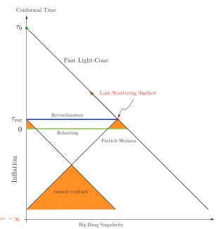
Despite the breathtaking diversity in structure at planetary and galactic scales, the universe is remarkably homogeneous at the largest scales. The homogeneity of the observable universe is one of the key observational puzzles of modern cosmology. In the standard big-bang model, patches in the sky that are larger than 2 degrees across in angular size should be causally independent and hence cannot thermalize. However, observations of the Cosmic Microwave Background (CMB) by Penzias & Wilson (Penzias & Wilson 1965) showed that the CMB was remarkably smooth on large scales. In fact the CMB, which traces the matter distribution in the early universe, is homogeneous to better than one part in 10,000. This remarkable smoothness of the CMB at the largest scales is known as the horizon problem. Figure 2.1 illustrates the horizon problem schematically in the standard cosmological model.

A second puzzle in observational cosmology is that the total energy density of the universe is almost equal to the critical energy density. There is no natural physical explanation for this value in the standard big-bang model and it leads to what is known as theflatness problem. In a series of papers in the early 1980s (Guth 1981; Albrecht & Steinhardt 1982; Linde 1982), it was hypothesized that a period of exponential expansion in the earliest stages of the universe, known asinflationcan solve both of these puzzles. The idea postulated that a new scalar field in the very early universe could drive this exponential expansion. Inflation would thus take a small, causally connected patch in the very early universe and expand it to the size of the observable universe.

(28)

Past Light-Cone

Recombination

Particle Horizon Conformal Time

Last-Scattering Surface

Big Bang Singularity

τrec τ0

τi= 0

Figure 2.1: Conformal diagram for standard FRW cosmology. In standard cosmol-ogy there are ∼ 105 causally disconnected patches (figure adopted from Baumann 2009).

In this chapter we aim to provide a brief review of inflationary physics starting with the homogeneous background evolution during inflation and the generation of perturbations. We also discuss the the proposed experimental tests of inflation using CMB polarization. The formalism outlined in this chapter will provide useful background for our discussion in Chapter IV. Details of the calculations outlined in this chapter can be found in standard textbooks (eg: Dodelson 2003) or review articles (see for eg Kamionkowski & Kovetz 2016).

2.1 The Physics of Inflation: Homogenous Evolution

An expanding homogeneous and isotropic Universe can be described by a Friedmann-Robertson-Walker (FRW) metric at the largest scales:

ds2 =−dt2+a2(t)

dr2

1−kr2 +r 2_d_Ω2

(2.1)

where a(t) is the scale factor parametrizing the background expansion rate. The growth rate of the universe (Hubble parameter) is given by,

H ≡ aÛ

a (2.2)

Assuming the evolution of the universe at the largest scales is governed by general relativity, the equation of motion for the scale factor is given by the Friedmann equations:

H2= ρ 3M_pl2 H+

Û

H2= −ρ+3p

(29)

Past Light-Cone

Recombination

Particle Horizon

Conformal Time

Last-Scattering Surface

Big Bang Singularity Reheating

causal contact

Inflation

τrec

τ0

0

τi=−∞

Figure 2.2: Inflation extends conformal time to negative values. The end of inflation is atτ= 0. As we can see in the figure, causally disconnected patches atτ= 0 were in causal contact before inflation (figure adopted from Baumann 2009).

where pand ρare the density and pressure of the background stress-tensor, which is assumed to be a perfect fluid. This is a valid assumption for a universe which is dominated by dark matter. Here we assume ~ = c = 1, Newton’s constant

G= 1/(8πMPl)2, and Planck mass,MPl =2.435×1018GeV.

Conformal Time and Causal Structure

We now turn to the kinematics of light-rays in the FRW metric- the kinematics of light- or null curves- determines the causal structure of the FRW spacetime. Null curves are defined by the conditionds2=0. They are easier to describe in terms of theconformal timethat is defined as1,

τ= ∫ dt

a(t) (2.4)

1_{note that conformal time is sometimes denoted by}_η_{(as we do in Chapter IV). However,}_η_is

used to denote one of the the slow-roll parameters in this chapter hence the use ofτfor conformal

(30)

With this definition, and assuming spatial isotropy, we can write the FRW metric as,

ds2= a2(τ)[−dτ2+dχ2] (2.5) which is the Minkowski metric scaled by a time-dependent conformal factor a(τ). In the metric defined by Eq. 2.5, light-rays travel in straight lines at ±45◦ in the

τ−χplane, making it easy to understand the causal structure of an isotropic, curved spacetime like the FRW metric.

Another quantity of interest is the the maximal comoving distance that light can travel between two timesτ1andτ2, known as the(comoving) particle horizon. The size of the particle horizon from a given spacetime point determines the causally connected region of spacetime,

χ(τ)=τ−τi =

∫ t

ti

dt

a(t) (2.6)

The particle horizon whereticorresponds to the big-bang singularity (i.e. a(t)=0)

can be written as

τ= ∫ t

0 dt a(t) =

∫

(aH)−1dlna (2.7)

The conformal time is thus proportional to (though not equal to) the comoving Hubble radius(aH)−1.

Inflation: Kinematics

The dynamics of the universe during the radiation and matter dominated stage is governed by,

d dt(aH)

−1 _>₀ _(2.8)

which implies that an observer in an expanding background will see a growing horizon of size H−1. In this case more information enters the horizon as time progresses.

For background evolution during inflation, this condition is reversed, i.e. d/dt(aH)−1< 0, which leads to ashrinking Hubble sphereand an exponentially growing scale fac-tora(t) ∝eHt.

We define the equation of state parameter as,

w ≡ p

(31)

φ φ

V(φ) V(φ)

Figure 2.3: Inflation postulates that the energy density of the universe is dominated by the vacuum energy associated with the displacement of a scalar field (the inflaton). The inflaton potential is unknown and needs to be constrained by observations. Here, shown for illustration are two toy models for the inflaton potential from ((figure adopted from Kamionkowski & Kovetz 2016)).

Defining ≡ − ÛH/H2, Friedmann equations imply,

= 3

2(1+w) (2.10)

Inflation thus requires thatw < −1/3.

Inflation: Dynamics

The equation of state necessary for inflation comes from the a hypothesized scalar fieldφcalled the "inflaton" with an associated potentialV(φ)(see Figure 2.3). During inflation, the stress-energy tensor of universe is dominated by the scalar field and it sources the evolution of the FRW background. We now set out to determine the conditions under which the scalar field can lead to accelerated expansion. The pressure and energy density components of the stress-energy tensor are given by,

p= Û

φ2

2 −V(φ) ; ρ= Û

φ2

2 +V(φ) (2.11)

The corresponding Friedmann equation governing time-evolutionφis given by,

Ü

φ+3HφÛ+∂φV(φ)= 0 (2.12) Note that here the potential acts like adriving force ∂φV(φ)while the expansion of the universe acts like africtiontermHφÛ.

We now define two quantities (called the slow-roll parameters) as,

≡ − Û H H2 =

Û

φ2

2M_pl2H2 (2.13)

and

η = Û

(32)

For inflation to occur both, η < 1.

We now make two approximations to simplify the equation of motion (Eq. 2.12). First, we assume that << 1 implying φÛ2/2 <<V(φ), leading to a simplification of the Friedmann equation to,

H2 ≈ V

3M_pl2 (2.15)

This implies that the Hubble rate during inflation is determined entirely by the inflaton potential. The second assumption we impose isη << 1, which simplifies the equation of motion (Eq. 2.12) to,

3HφÛ≈ −∂_φV(φ) (2.16) We thus have reduced a second order equation of motion to a first order equation, needing us to specify only one initial condition.

Together these two conditions are known as theslow roll approximationwhich can be summarized as,

≈ MPl2 2

∂

φV

V(φ) 2

<<1 (2.17)

and

η=−2 Û H H2 −

Û

2H <<1 (2.18)

2.2 The Physics of Inflation: Generation of Perturbations

In this section we provide a brief discussion of the generation of primordial density and tensor perturbations from quantum fluctuations during inflation. The discussion does not delve into the technical details of the calculation (for details see Baumann 2009). Instead we provide a heuristic outline for the calculation.

Scalar Perturbations

Consider a scalar field φ that varies in space and time. Since the energy density is dominated by φ, spatial fluctuations in φwill lead to spatial fluctuations in the energy density which will induce fluctuations in the spacetime metric.

The perturbations for the scalar field and the metric during inflation are given by,

(33)

where

ds2 = gµνdxµdxν

= −(1+2Φ)dt2+2aBidxidt+a2[(1−2Ψ)δi j+Ei j]dxidxj (2.20)

The metric perturbations can be decomposed into Scalars, Vectors, and Tensors (the SVT decomposition), given by,

Bi ≡ ∂iB−Si, (2.21)

where

∂i

Si =0, (2.22)

and

Ei j ≡2∂i jE+2∂(iFj)+hi j, (2.23)

where

∂i

Fi = 0, hi_i =∂ihi j = 0. (2.24)

We ignore the vector perturbations, Si and Fi since they decay with the expansion

of the universe. Instead we focus on the scalar and tensor modes.

An important characteristic of perturbations in GR are that they are not unique, but depend on the choice of coordinates or gauge. Note that tensor fluctuations are gauge-invariant, but scalar fluctuations depend on the choice of gauge. We choose a gauge defined by vanishing momentum density i.e. δT0i = 0 which corresponds

toδφ=0. This is known as thecomoving gauge. The scalar metric (to linear order in perturbation theory) can be written as,

g0ν =0 ;gi j = a2(t)exp[2ζ( ®x,t)]δi j (2.25)

where ζ( ®x,t) is the curvature perturbation. The φ = 0 comoving spatial surfaces have a three-curvature ofR(3) =4/a2∇2ζ and henceζis referred to as thecomoving

curvature perturbation. It can be shown that ζ is conserved on super-horizon scales for adiabatic fluctuations irrespective of the equation of state of the matter. This provides an essential link between the fluctuations created during inflation and observables in the late universe.

The non-dynamical metric perturbations δg00 and δg0i are further related to ζ

(34)

through constraint equations and how it can be used to compute the second-order action for the comoving curvature perturbation in quadratic order inζ.

For the slow-roll model described earlier, the action is given by,

S= 1 2

∫

d4x√−g R− (∇φ)2−2V(φ) , (2.26) Our goal is to compute the perturbations of this action due to fluctuations in the scalar field and the metric in the ADM formalism. In the ADM formalism the spacetime is sliced into three-dimensional hypersurfaces given by

ds2=−N2dt2+gi j(dxi+ Nidt)(dxj+Njdt). (2.27)

where gi j is the three-dimensional spatial metric on constant t-slices. The lapse

functionN(x)and the shift functionNi(x)contain the same information as the metric

perturbationsΦandB. They correspond to non-dynamical Lagrange multipliers in the action. In the ADM formalism, the action can be written as,

S = 1 2

∫

d4x√−ghN R(3) −2NV+N−1(Ei jEi j−E2)+

N−1( Ûφ−Ni∂iφ)2−Ngi j∂iφ∂jφ−2V

i

, (2.28)

where

Ei j ≡

1

2( Ûgi j − ∇iNj − ∇jNi), E = E

i

i . (2.29)

Ei j is related to the extrinsic curvature of the three-dimensional spatial slicesKi j =

N−1Ei j.

The ADM action given in Eqn.(2.28) leads to the constraint equations for the Lagrange multipliersN andNi,

∇_i[N−1(Ei_j −δi_jE)]= 0, (2.30) R(3)−2V −N−2(Ei jEi j −E2) −N−2φÛ2= 0. (2.31)

To solve the constraints, we split the shift vectorNiinto scalar and vector components

Ni ≡ψ,i+N˜i, wher e N˜i,i = 0, (2.32)

and define the lapse perturbation as

(35)

(36)

(37)

(38)

(39)

(40)

CMB Temperature Anisotropies

We now discuss the we the evolution of perturbations after the modes re-enter the horizon and eventually become the anisotropies we observe in the CMB. In this section we outline the essential machinery needed to translate the primordial fluctuations to the observed CMB spectrum.

After entering the horizon, the curvature perturbations lead to density fluctuations in the primordial plasma. As the universe cools, the formation of neutral hydrogen leads to the photons decoupling. These photons get redshifted and are observed today as CMB photons. The CMB anisotropies thus contains information about the primordial density perturbations.

The measured CMB temperature fluctuation map on the sky can be expanded in terms of spherical harmonics,

Θ(n) ≡ˆ δT(nˆ)

T =

Õ

`m

a`mY`m(n)ˆ , (2.61)

where,

a`m =

∫

dΩY_`m∗ (n)ˆ Θ(n)ˆ . (2.62) Here, Y`m(nˆ) are the standard spherical harmonics on a 2-sphere. The statistical isotropyof the universe allows us to define the angular power spectrum of the CMB in terms of the the multipole momentsa`m as,

C_`TT = 1 2`+1

Õ

m

ha∗_`ma`mi ; ha_`m∗ a`0_m0i=CTT_` δ_``0δ_mm0, (2.63)

CMB temperature fluctuations are dominated by the scalar modes ζ. The linear evolution which relatesζand temperature anisotropies is determined by the transfer function∆T`(k)through thek-space integral

a`m = 4π(−i)` ∫

d3k

(2π)3∆T`(k)ζkY`m(kˆ) (2.64) Moreover, we can write down the power spectrum of the curvature fluctuations as,

(41)

(42)

Figure 2.5: Current constraints on the scalar spectral indexns and tensor-to-scalar

ratior, for a variety of slow-roll inflationary models. Figure adopted from Planck Collaboration et al. 2016.

The CMB is polarized because free electrons during recombination see an anisotropic radiation field sourced by primordial density fluctuations. The linear polarization arises due to the quadrupole of the radiation field incident on an electron (in its rest frame). The CMB polarization thus encodes information about the primordial density (or scalar) fluctuations.

Since polarization is not a scalar field, the standard decomposition in terms of spherical harmonics as discussed in the previous section is no longer applicable. Linear polarization is then described by the Stokes parametersQ= 1₄(I11−I22)and U = 1₂I12, whereIi j(nˆ)is the 2×2 intensity tensor. Here ˆndenotes the direction on

the sky. The components ofIi jare defined relative to two orthogonal basis vectors ˆe1 and ˆe2perpendicular to ˆn. The polarization magnitude and angle areP =

p

Q2+_U2 and α = 1₂tan−1(U/Q). The temperature anisotropy is given byT = 1₄(I11+ I22) and is invariant under a rotation in the plane perpendicular to ˆn. Therefore the temperature field can be expanded in terms of scalar (spin-0) spherical harmonics.

The quantities Q and U, transform under rotation by an angle ψ as a spin-2 field (Q±iU)(nˆ) → e∓2iψ(Q±iU)(nˆ). The harmonic analysis ofQ±iUtherefore requires expansion on the sphere in terms of tensor (spin-2) spherical harmonics

(Q±iU)(n)ˆ =Õ

`,m

(43)

E-mode Polarization

l

-25 -20 -15 -10 -5 0 5 10 15 20 25

b

-5

0

5

B-mode Polarization

l

-25 -20 -15 -10 -5 0 5 10 15 20 25

b

-5

0

5

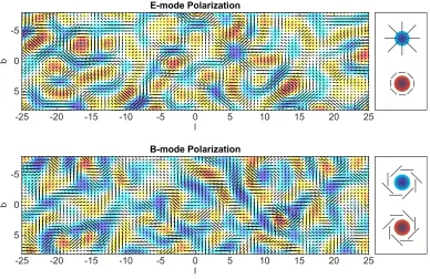
Figure 2.6: The top panel shows a polarization pattern composed only ofE modes. The polarization pattern is tangential around hot spots and radial around cold spots. The bottom panel shows a polarization pattern composed only of B modes. The polarization pattern surrounding hot and cold spots of theBmode show a swirling pattern. Note that the E-mode is parity invariant while the B-mode is not. Figure adopted from Kamionkowski & Kovetz 2016.

We now introduce linear combinations of the momentsa±2,`m, aE,`m ≡ −1

2 a2,`m +a−2,`m _,

aB,`m ≡ −1

2i a2,`m−a−2,`m _.

(2.71)

This allows us to define two spin-0 fields instead of the spin-2 quantitiesQandU E(n)ˆ = Õ

`,m

aE,`mY`m(n)ˆ , B(n)ˆ =

Õ

`,m

aB,`mY`m(n)ˆ . (2.72)

The scalar quantities E and B completely describe a linear polarization field. E-mode polarization iscurl-freewith polarization vectors pointing radially around cold spots and tangentially around hot spots. B-mode polarization isdivergence-freebut has acurl: the polarization vectors have a net vorticity around any given point on the sky (see Fig. 2.6).

(44)

(45)

2.4 Conclusion

Measurement of the B-modes of the CMB is the most promising strategy to detect inflationary gravitational waves in the immediate term. One of the caveats for the detectability of inflationary gravitational waves is that their strength (determined by r) depends on the (hitherto unknown) model of inflation. Models of single-field slow-roll (SFSR) inflation predict a range of values of r, from order unity to very low values. While models that predict r of order unity are already ruled out by observations, power-law inflationary potentials that predictr of the order of 1−ns are the most interesting to immediate term CMB experiments. On the other

hand, Higgs-like potentials can lead tor ∼ 0.001 which can be probed by the next generation of CMB experiments. SFSR models with very flat potentials, where inflation ends when the inflation falls off a cliff (for example, the second panel in Fig.2.3), can lead to very low values ofrand these are not likely to be detected even with the next generation CMB experiments.

While there is no broad consensus on “natural” models of inflation, given the mea-surements of the scalar spectral indexns, SFSR models with power-law potentials

that predict values of r ∼ 0.01 can potentially be detected by ground-based CMB experiments over the next decade. Note that the measurement ofr will enable us to directly measure the energy scale of inflationV_i1_{n f}/4 ∼10−3(r/0.01)1/4MPl, where

MPlis the Planck mass.

The current upper bounds on r from the combination of the CMB B-mode and other observables arer < 0.07 (95% CL) (BICEP2 Collaboration et al. 2016). The measurement of the scalar spectral indexns by Planck rules out very low values of

r (r < 10−4) for many of the simplest models, although model dependency implies one could get lower values ofrin special cases (see Kamionkowski & Kovetz 2016 for a discussion on inflationary models that predict low values of r). Measuring B-modes at ther > 0.002 level is the goal of future CMB “Stage-IV” experiments (Abazajian et al. 2016). However, for low values of r CMB B-mode experiments need to confront challenging Galactic foregrounds and the contaminating lensing signal. In the event of a detection it will be crucial to verify the result using techniques that have independent systematics.

(46)

at high-frequencies with a network of space-based laser interferometers has also been proposed (Corbin & Cornish 2006; Kawamura et al. 2011). In Chapter 4 we propose a new technique to detect inflationary gravitational waves using the circular polarization of the 21 cm line. This technique, while futuristic, has the potential to prober ∼10−5using an array of closely packed dipole antennas with a side length of 1000 km. In the event that near-term CMBB-mode experiments measure a value ofr, our technique could potentially be used to verify the detection. In the case that the value ofr < 10−3, our technique would be a viable way to probe inflationary gravitational waves at lowr.

References

Abazajian, K. N., Adshead, P., Ahmed, Z., et al., 2016, ArXiv e-prints

Albrecht, A., & Steinhardt, P. J., 1982, Physical Review Letters, 48, 1220

Alizadeh, E., & Hirata, C. M., 2012, PhRvD, 85.12, 123540, 123540

Baumann, D., 2009, ArXiv e-prints

BICEP2 Collaboration, Keck Array Collaboration, Ade, P. A. R., et al., 2016, Phys-ical Review Letters, 116.3, 031302, 031302

Chisari, N. E., Dvorkin, C., & Schmidt, F., 2014, PhRvD, 90.4, 043527, 043527

Corbin, V., & Cornish, N. J., 2006, Classical and Quantum Gravity, 23, 2435

Dodelson, S. 2003, Modern cosmology

Dodelson, S., Rozo, E., & Stebbins, A., 2003, Physical Review Letters, 91.2, 021301, 021301

Guth, A. H., 1981, PhRvD, 23, 347

Guth, A. H., & Pi, S.-Y., 1982, Physical Review Letters, 49, 1110

Hanson, D., Hoover, S., Crites, A., et al., 2013, Physical Review Letters, 111.14, 141301, 141301

Hawking, S. W., 1982, Physics Letters B, 115, 295

Kamionkowski, M., Kosowsky, A., & Stebbins, A., 1997, Physical Review Letters, 78, 2058

Kamionkowski, M., & Kovetz, E. D., 2016, ARA&A, 54, 227

Kawamura, S., Ando, M., Seto, N., et al., 2011, Classical and Quantum Gravity, 28.9, 094011, 094011

Linde, A. D., 1982, Physics Letters B, 108, 389

(47)

Planck Collaboration, Ade, P. A. R., Aghanim, N., et al., 2016, A&A, 594, A20, A20

Rubakov, V. A., Sazhin, M. V., & Veryaskin, A. V., 1982, Physics Letters B, 115, 189

Schmidt, F., & Jeong, D., 2012, PhRvD, 86.8, 083513, 083513

Schmidt, F., Pajer, E., & Zaldarriaga, M., 2014, PhRvD, 89.8, 083507, 083507

Seljak, U., & Zaldarriaga, M., 1997, Physical Review Letters, 78, 2054

(48)

C h a p t e r 3

OVERVIEW OF 21CM COSMOLOGY

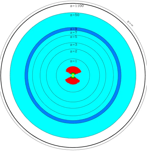
The distribution of matter approximately 400,000 years after the Big Bang has been exquisitely measured using the statistics of the CMB. The first stars and galaxies formed within the first billion years of the universe and led to the formation of the complex cosmic web that has been probed by galaxy surveys over the past two decade. However, both the CMB and galaxy surveys map out a small fraction of the universe’s comoving volume. As seen in Figure. 3.1, a large volume of the universe remains unexplored by current cosmological probes.

The epoch of the universe after recombination and before the first galaxies formed is often referred to as the Cosmic Dark Ages, since the universe was mostly neutral and gravity was the dominant force governing the evolution. Probing the Dark Ages will provide access to a large number of modes in the matter distribution of the universe, allowing us to put stringent constraints on cosmological parameters. It will also allow us to understand the phase transition of the universe from an almost neutral state to a completely ionized state, due to the first stars and galaxies.

The efforts to probe the dark ages rely on the observation of low-frequency radio emission from the hyperfine transition of neutral hydrogen. The interaction between the proton and electron spins in neutral hydrogen leads to a splitting of the ground state of neutral hydrogen. Transition between these hyperfine states leads to the emission of a photon with a wavelength of about 21cm. The emitted 21cm photon is then redshifted due to the expansion of the universe. For a given model of the expansion of the universe we can thus observe different redshifts or distances by tuning the frequency. Using multi-frequency radio experiments, we can thus construct 3D, tomographic maps of the universe during the dark ages.

(49)

Figure 3.1: 21 cm observations can potentially map the largest volumes of the observable universe, while the CMB can probe a 2D surface atz ∼1100. and LSS surveys can map small volumes of the local universe. Note that more than half of the comoving volume of the universe lies atz> 20. Figure adopted from Tegmark & Zaldarriaga 2009.

3.1 Physics of the 21cm Signal

21cm cosmology is made possible due to a simple radiative process in the early universe: the CMB acts as a backlight for neutral hydrogen atoms in the high-redshift IGM leading to absorption or emission of the 21 cm line. To describe the 21cm signal, we typically use the specific intensity Iν at a given frequency ν. For

low-frequencies we can use the Rayleigh-Jeans limit of the blackbody spectrum to relateIν to the brightness temperatureTbvia,

Iν ≡ 2kbTbν

2

c2 . (3.1)

The radiative transfer equation for hydrogen atoms at redshiftzbacklit by the CMB with temperatureTγ(z)can then be written as,

(50)

Hereτν is the the optical depth of the cloud due to the hyperfine transition andTsis

the spin temperature defined by,

n(F =1) n(F =0) =

g1

g0

exp[−T∗ Ts

] (3.3)

, where F = 0 denotes the spin-antiparallel hyperfine level, F = 1 denotes the spin-parallel level,g1 =3 andg0= 1 are the statistical weights andT∗ =~ωh f/kB =

68mK is the hyperfine splitting in temperature units. We observe 21cmemissionif Ts > Tγ and absorption ifTs <Tγ.

The optical depth along a line of sight of a hydrogen cloud is given by,

τν =

∫

dl[(1−exp(−E10/kBTs)]σ0φ(ν)n0 (3.4) , where n0 = nH/4, nH being the hydrogen density and the 21cm cross-section is

given by σ(ν) = σ₀φ(ν), with σ0 ≡ 3c2A10/8πν2, where A10 is the spontaneous decay rate of the spin-flip transition, and the line profile is normalized by,

∫

φ(ν)dν =1 (3.5)

To evaluate the optical depth we need to determine the path length as a function of frequencyl(ν)which determines the range of frequencies dν over the path dl that corresponds to a given observed frequency νobs. This is done using the Sobolev approximation that assumes a linear velocity profile locallyv = (dv/dl)l and then using the Doppler shifted frequencyνobs =νem(1−v/c).

The spin temperature depends on three processes:

• Absorption or stimulated emission of CMB photons near the 21cm transition. This leads to a coupling betweenTs andTγ

• Collisional excitation and de-excitation of hydrogen atoms. These include hydrogen collisions, electron collisions, and hydrogen-proton collisions. This leads to a coupling between Ts and the kinetic gas

temperatureTk

(51)

Figure 3.2: The transitions relevant for the Wouthuysen-Field effect. Solid line transitions contribute to spin flips. Transitions denoted by dashed lines are allowed but do not contribute to spin flips. Figure adopted from Pritchard & Loeb 2012.

The Wouthuysen-Field effect is illustrated in Figure 3.2. The figure shows the hyperfine 1S and 2P levels or hydrogen. If the hydrogen is initially in the hyperfine singlet state, the absorption of a Lyα photon will excite it to either of the central 2P hyperfine states. The other two hyperfine states are inaccessible due to selection rules. The subsequent emission of a Lyαphoton can bring the atom back to either of the two ground state hyperfine levels. In the case when the atom transitions to the triplet state, a spin-flip takes place. Thus resonant scattering of Lyαphotons can lead to a spin flip.

The Wouthuysen-Field effect couples the spin temperature Ts to the color

(52)

Figure 3.3: The evolution of the 21 cm global signal depends on different physical processes at different epochs. The evolution of the brightness temperatureTbleads

to the 21cm signal appear either in absorption or in emission against the CMB. The top panel shows a slice through a simulation showing the evolution ofTband the

heating due to the first generation stars and galaxies. The bottom panel shows the sky-averaged global 21 cm signal, which largely traces the evolution of the spin temperature and neutral fraction of hydrogen. Figure adopted from Pritchard & Loeb 2012.

into local equilibrium, for frequencies near the line center. This leads toTLyα ≈Tk.

In equilibrium, the spin temperature is given by,

T_s−1 = T

−1

γ +xcT_K−1+xαTα−1

1+ xc+xα

, (3.6)

where xc is the collisional coupling coefficient and xα is the Lyman-α coupling

coefficient. Note that these are not fundamental parameters but instead depend on cross-sections as well as macro-physics parameters like gas density and Lyα intensity

Observationally, we are interested in the brightness temperature of the 21cm line. Quantum mechanically, the 21 cm transition is a forbidden transition, with a lifetime for spontaneous emission of∼ 3×107years. Thereforeτνis small and we can work in the optically thin regime. The brightness temperature fluctuation relative to the CMB at redshift z in the optically thin limit is given by

δTb(rˆ, ν) ≈27xH

Ts −Tγ

Ts

1+z 10

1/2

(1+δb)(1+δx)

(1+z)H(z)

∂||v||

(53)

where ˆr is unit direction vector, xH is the mean neutral hydrogen fraction,v|| is the

velocity along the line-of-sight direction, δb is the fractional baryon overdensity,

andδx is the neutral fraction overdensity. The variation of these parameters across

space and along redshift leads to a rich 3D field of the 21cm brightness temperature. The statistics of this brightness temperature field encapsulate both fundamental cosmological parameters as well as astrophysics during the Dark Ages.

3.2 Evolution of the 21cm Signal

The evolution of the brightness temperatureTbacross frequency, and hence across

redshift, depends on both cosmological parameters (eg: the matter power spectrum), as well as more complex astrophysical qualities (e.g., the Lyman-αflux), as evident from Eqn 3.7. The evolution of the spatially averaged, "global" 21cm signal is shown in Figure 3.3 (adapted from Pritchard & Loeb 2012). Future 21cm experiments will thus need to construct high-resolution maps ofTbacross multiple redshifts.

Meaningful cosmological information from the maps can only be extracted statisti-cally. The quantity of interest is the power spectrum of the brightness temperature field, defined as,

hTˆ_b∗(k)Tˆb(k0)i = (2π)3δ(k−k0)PT(k), (3.8)

where ˆTbis the 3D spatial Fourier transform of theTbfield. The angle brackets denote

an ensemble average and δ(k− k0) is the Dirac delta function. For a statistically isotropic 21cm signal,P(k)is the same asP(k). We also define,

∆2₂₁(k)= k 3

2π2P(k), (3.9)

which measures the contribution to the root-mean-square fluctuations in Tb per

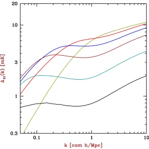
logarithmic bin in k. We plot different theoretical models of∆2₂₁(k)corresponding to different ionization fractions of the IGM in Figure. 3.4.

The power spectrum of the brightness temperature is a redshift dependent quantity. Here we summarize the different regimes and the key physical processes at play:

• High Redshifts (40<z<200): Compton scattering of the residual free electrons after recombination leads to thermal coupling of the gas to the CMB at z > 200, and this leads to a tight coupling betweenTγ, Tk andTs and they

(54)

Figure 3.4: The evolution of the 21 cm power spectrum as a function of the ionized fraction is expected to reveal the astrophysical processes that drove reionization and the nature of the first stars and galaxies. The right side of the y-axis shows neutral fraction of the universe. As the universe goes from almost neutral (yellow) to ionized (gray), the overall amplitude of the power spectrum decreases. Moreover, as reionization proceeds the high-kpower decreases since reionization bubbles start forming at small scales and then grow to larger scales.

After z ∼ 200, the gas begins to cool adiabatically: Tk ∝ (1+ z)2 while the

CMB temperatureTγ ∝ (1+z). This setsTγ > Ts and the signal appears in

absorption until z ∼ 40 when collisional coupling stops becoming effective. During this period the 21cm fluctuations are sourced purely by the dark matter distribution and measurement of the 21cm power spectrum during this epoch can enable us to probe the matter power spectrum with exquisite precision.

(55)

the ionizing sources. These UV photons have a very short mean free path in the neutral medium and lead to ionized HII regions with a sharp boundary. Photons with 10.2 < E < 13.6 eV redshift until they enter a Lyman series resonance and subsequently generate Lyαphotons via atomic cascades. The Lyαphotons couple toTs via the Wouthuysen-Field effect.

Since the neutral fraction in the universe is still high, Tα is almost equal

to Tk, leading to a second dip in the global signal and the 21 cm signal

becoming visible in absorption. The heating of the IGM due to the first x-ray sources leads to Tk becoming more thanTγ, which leads to 21cm emission

from certain parts of the IGM. The spatial structure of the 21cm field is thus far more complex during this epoch and depends on the Lyman-αfield, the distribution of x-ray sources and the background evolution of dark matter. Note that the scattering of Lyαphotons off hydrogen atoms is rather inefficient in heating the gas- the spectral distortion of the Lyαphotons during scattering greatly reduces the heating rate. Hence Lyαheating requires very large Lyα fluxes and is likely to be more efficient at later times. On the other hand X-ray heating of the gas is likely to be very efficient during this epoch. X-ray photons have a very long mean free path, and hence are able to heat the gas at greater distances from the source,. Moreover, X-rays can be produced in large quantities once the first compact objects are formed. X-rays heat the gas primarily through ionization. Heating happens via energetic photo-electrons generated due to photo-ionization that dissipate their energy through heating the gas.

Aroundz∼ 10 ultraviolet photons from the first generation of high-mass stars start "re-ionizing" the universe. This leads to growing "bubbles" of ionized material, centered on the most luminous objects, that eventually grow in size and coalesce. During reionization the power shifts from high-k scales to low-k scales since the ionized fraction is low at large scales, leading to a higher 21cm signal (there is no 21cm signal from the ionized bubbles). Studying the power spectrum as a function of redshift can thus allow us to constrain the process of reionization and understand the first luminous sources

(56)

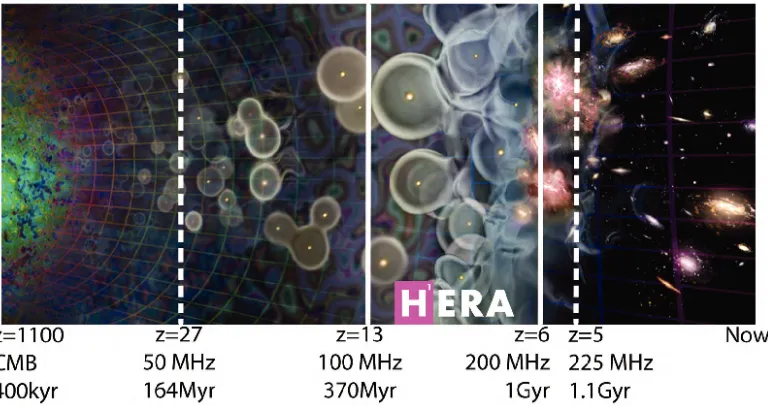
Figure 3.5: The evolution of the universe from the CMB (extreme left) to the current day (extreme right). After the CMB the universe goes through the Dark Ages when it is largely neutral. As the first stars and galaxies light up, the universe gets reionized. Reionization is inhomogeneous and fills the the universe with merging bubbles of ionized hydrogen. Image credit: HERA/Avi Loeb/SciAm

(57)

(58)

(59)

Figure 3.6: Schematic of a two antenna interferometer.

experiments (see, e.g., Refs. Mao et al. 2008; Furlanetto et al. 2009; Pober et al. 2014; Mao et al. 2008).

A schematic of the experimental setup considered here is shown in Fig. 3.6. Modes with frequencies that differ by less than 1/t1cannot be distinguished, and modes with frequencies in each interval 1/t1are collapsed into a discrete mode with frequency

νn = n/t1, where n ∈ Z. Thus, the number of measured (discrete) frequencies is

Nν =t1∆ν. Electric field induced in a single antenna is

E(t)=

Nν

Õ

n

e

E(νn)e2πiνnt, (3.15)

while the quantity an interferometer measures is the correlation coefficient between the electric fieldEiin one and the electric fieldEjin the other antenna, as a function

of frequency,

ρi j(ν) ≡

hEe_i∗(ν)Eej(ν)i

q

h|Eei(ν)|2ih|Eej(ν)|2i

. (3.16)

Let us now assume that

hEe

∗

(60)

(61)

(62)