International Journal of Scientific Research in Computer Science, Engineering and Information Technology © 2017 IJSRCSEIT | Volume 2 | Issue 4 | ISSN : 2456-3307
A Survey of Routing Strategy for Ad Hoc Network
M. Nellaiappan, R. Lydia Jascinth Femila, S. Padmavathy
Prince Shri Venkateshwara Padmavathy Engineering College, Chennai, Tamil Nadu, India
ABSTRACT
The 1990s have seen a rapid growth of research interests in mobile ad hoc networking. The infrastructureless and the dynamic nature of these networks demands new set of networking strategies to be implemented in order to provide efficient end-to-end communication. This, along with the diverse application of these networks in many different scenarios such as battlefield and disaster recovery, have seen MANETs being researched by many different organisations and institutes. MANETs employ the traditional TCP/IP structure to provide end-to-end communication between nodes. However, due to their mobility and the limited resource in wireless networks, each layer in the TCP/IP model require redefinition or modifications to function efficiently in MANETs. One interesting research area in MANET is routing. Routing in the MANETs is a challenging task and has received a tremendous amount of attention from researches. This has led to development of many different routing protocols for MANETs, and each author of each proposed protocol argues that the strategy proposed provides an improvement over a number of different strategies considered in the literature for a given network scenario. Therefore, it is quite difficult to determine which protocols may perform best under a number of different network scenarios, such as increasing node density and traffic. In this paper, we provide an overview of a wide range of routing protocols proposed in the literature. We also provide a performance comparison of all routing protocols and suggest which protocols may perform best in large networks
Keywords : Routing, Adhoc, MANET, protocols, Distance vector, Link state
I.
INTRODUCTION
1. Classification of current routing protocols
The limited resources in MANETs have made designing of an efficient and reliable routing strategy a very challenging problem. An intelligent routing strategy is required to efficiently use the limited resources while at the same time being adaptable to the changing network conditions such as: network size, traffic density and network partitioning. In parallel with this, the routing protocol may need to provide different levels of QoS to different types of applications and users.Prior to the increased interests in wireless networking, in wired networks two main algorithms were used. These algorithms are commonly referred to as the link-state and distance vector algorithms. In link-state routing, each node maintains an up-to-date view of the network by periodically
broadcasting the link-state costs of its neighbouring nodes to all other nodes using a flooding strategy. When each node receive an update packet, they update their view of the network and their link-state information by applying a shortest-path algorithm to choose the next hop node for each destination. In distance-vector routing, for every destination x, each node i maintains a set of distances Dx
ij where j ranges
over the neighbours of node i. Node i selects a neighbour, k, to be the next hop for x if Dx
ik=minj{Dxij}.
require each node to frequently recharge their power supply.To overcome the problems associated with the link-state and distance-vector algorithms a number of routing protocols have been proposed for MANETs. These protocols can be classified into three different groups: global/proactive, on-demand/reactive and hybrid. In proactive routing protocols, the routes to all the destination (or parts of the network) are determined at the start up, and maintained by using a periodic route update process. In reactive protocols, routes are determined when they are required by the source using a route discovery process. Hybrid routing protocols combine the basic properties of the first two classes of protocols into one. That is, they are both reactive and proactive in nature. Each group has a number of different routing strategies, which employ a flat or a hierarchical routing structure.
II.
METHODS AND MATERIAL
2. Proactive Routing Protocols
In proactive routing protocols, each node maintains routing information to every other node (or nodes located in a specific part) in the network. The routing information is usually kept in a number of different tables. These tables are periodically updated and/or if the network topology changes. The difference between these protocols exist in the way the routing information is updated,1 detected and the type of information kept
at each routing table. Furthermore, each routing protocol may maintain different number of tables. This section describes a number of different proactive protocols and makes a performance comparison between them. That is illustrated in Table 1 and Table 2. Note that the performance metrics represent the worst case scenario for each routing protocol
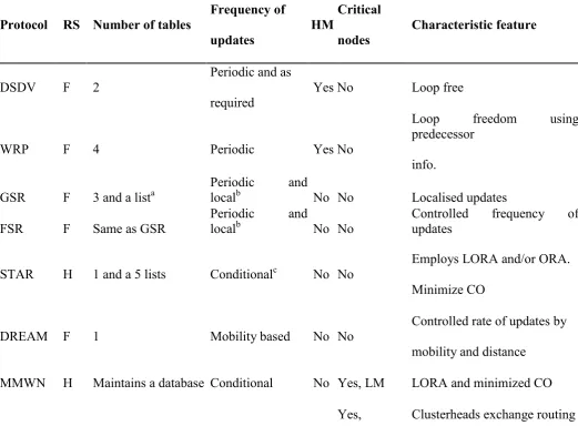
Table 1. Basic characteristics of proactive routing protocols
Frequency of
Critical
Protocol RS Number of tables
HM
Characteristic feature
updates
nodes
Periodic and as
DSDV
F
2
Yes No
Loop free
required
Loop
freedom
using
predecessor
WRP
F
4
Periodic
Yes No
info.
GSR
F
3 and a list
aPeriodic
and
local
bNo No
Localised updates
FSR
F
Same as GSR
Periodic
and
local
bNo No
Controlled
frequency
of
updates
Employs LORA and/or ORA.
STAR
H
1 and a 5 lists
Conditional
cNo No
Minimize CO
Controlled rate of updates by
DREAM F
1
Mobility based
No No
mobility and distance
MMWN H
Maintains a database Conditional
No Yes, LM
LORA and minimized CO
CGSR
H
2
Periodic
No
Clusterhead information
2 (link-state table
and
Periodic, within
Yes,
Low CO and Hierarchical
HSR
H
No
location management)
deach subnet
Clusterhead structure
3
(Routing,
neighbour
OLSR
F
Periodic
Yes No
Reduces CO using MPR
and topology table)
Periodic and
Yes, Parent Broadcasting topology updates
TBRPF
F
1 Table, 4 lists
Yes
differential
node
over a spanning tree
R=routing structure; HM=hello message; H=hierarchical; F=flat; CO=control overhead;
LORA=least overhead routing approach; ORA=optimum routing approach; LM=location
manager.
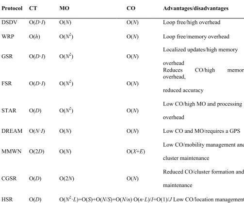
Table 2.
Complexity comparison of proactive routing protocols
Protocol CT
MO
CO
Advantages/disadvantages
DSDV
O(
D
·
I
)
O(
N
)
O(
N
)
Loop free/high overhead
WRP
O(
h
)
O(
N
2)
O(
N
)
Loop free/memory overhead
Localized updates/high memory
GSR
O(
D
·
I
)
O(
N
2)
O(
N
)
overhead
Reduces
CO/high
memory
overhead,
FSR
O(
D
·
I
)
O(
N
2)
O(
N
)
reduced accuracy
Low CO/high MO and processing
STAR
O(
D
)
O(
N
2)
O(
N
)
overhead
DREAM O(
N
·
I
)
O(
N
)
O(
N
)
Low CO and MO/requires a GPS
Low CO/mobility management and
MMWN O(2
D
)
O(
N
)
O(
X
+
E
)
cluster maintenance
Reduced CO/cluster formation and
CGSR
O(
D
)
O(2
N
)
O(
N
)
maintenance
Reduced CO and contention/2-hop
OLSR
O(
D
·
I
)
O(
N
2)
O(
N
2)
neighbour knowledge required
O(
D
)
or
D
+2 for
TBRPF
O(
N
2)+O(
N
)+O(
N
+
V
)
O(
N
2)
Low CO/High MO
link failure
CT=convergence time; MO=memory overhead; CO=control overhead; (1)=indicates that a fixed number of update tables is transmitted; V=number of neighbouring nodes; N=number of nodes in the network; n=average number of logical nodes in the cluster; I=average update interval; D=diameter of the network; S=number of virtual IP subnets;
h=height of the routing tree; X=total number of LMs (each cluster has an LM); J=nodes to home agent registration interval; L=number of hierarchical level.
2.1. Destination-sequenced distance vector (DSDV)
The DSDV algorithm [27] is a modification of DBF [3, 10], which guarantees loop free routes. It provides a single path to a destination, which is selected using the distance vector shortest path routing algorithm. In order to reduce the amount of overhead transmitted through the network, two types of update packets are used. These are referred to as a “full dump” and “incremental” packets. The full dump packet carries all the available routing information and the incremental packet carries only the information changed since the last full dump. The incremental update messages are sent more frequently than the full dump packets. However, DSDV still introduces large amounts of overhead to the network due to the requirement of the periodic update messages, and the overhead grows according to O(N2). Therefore the protocol will not
scale in large network since a large portion of the network bandwidth is used in the updating procedures.
2.2. Wireless routing protocol (WRP)
The WRP protocol [22] also guarantees loops freedom and it avoids temporary routing loops by using the predecessor information. However, WRP requires each node to maintain four routing tables. This introduces a
significant amount of memory overhead at each node as the size of the network increases. Another disadvantage of WRP is that it ensures connectivity through the use of hello messages. These hello messages are exchanged between neighbouring nodes whenever there is no recent packet transmission. This will also consume a significant amount of bandwidth and power as each node is required to stay active at all times (i.e. they cannot enter sleep mode to conserve their power).
2.3. Global state routing (GSR)
The GSR protocol [5] is based on the traditional Link State algorithm. However, GSR has improved the way information is disseminated in Link State algorithm by restricting the update messages between intermediate nodes only. In GSR, each node maintains a link state table based on the up-to-date information received from neighbouring nodes, and periodically exchanges its link state information with neighbouring nodes only. This has significantly reduced the number of control message transmitted through the network. However, the size of update messages is relatively large, and as the size of the network grows they will get even larger. Therefore, a considerable amount of bandwidth is consumed by these update messages.
2.4. Fisheye state routing (FSR)
accurate. This can be overcome by making the frequency at which updates are sent to remote destinations proportional to the level of mobility. This is discussed in more detail in Section 3.
2.5. Source-tree adaptive routing (STAR)
The STAR protocol [11] is also based on the link state algorithm. Each router maintains a source tree, which is a set of links containing the preferred paths to destinations. This protocol has significantly reduced the amount of routing overhead disseminated into the network by using a least overhead routing approach (LORA), to exchange routing information. It also supports optimum routing approach (ORA) if required. This approach eliminated the periodic updating procedure present in the Link State algorithm by making update dissemination conditional. As a result the Link State updates are exchanged only when certain event occurs. Therefore STAR will scale well in large network since it has significantly reduced the bandwidth consumption for the routing updates while at the same time reducing latency by using predetermined routes. However, this protocol may have significant memory and processing overheads in large and highly mobile networks, because each node is required to maintain a partial topology graph of the network (it is determined from the source tree reported by its neighbours), which may change frequently as the neighbours keep reporting different source trees.
2.6. Distance routing effect algorithm for mobility (DREAM)
The DREAM routing protocol [2] employs a different approach to routing when compared to the routing protocols described so far. In DREAM, each node knows its geographical coordinates through a GPS. These coordinates are periodically exchanged between each node and stored in a routing table (called a location table). The advantage of exchanging location information is that it consumes significantly less bandwidth than exchanging complete link state or distance vector information, which means that it is more scalable. In DREAM, routing overhead is further reduced, by making the frequency at which update messages are disseminated proportional to mobility and the distance effect. This means that stationary nodes do not need to send any update messages.
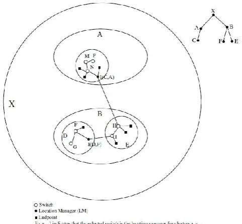
2.7. Multimedia support in mobile wireless networks (MMWN)
In MMWN routing protocol [20] the network is maintained using a clustering hierarchy. Each cluster has two types of mobile nodes: switches and endpoints. Each cluster also has location manager (LM), which performs the location management for each cluster (see Fig. 1). All information in MMWN is stored in a dynamically distributed database. The advantage of MMWN is that only LMs perform location updating and location finding, which means that routing overhead is significantly reduced when compared to the traditional table driven algorithms (such as DSDV and WRP). However, location management is closely related to the hierarchical structure of the network, making the location finding and updating very complex. This is because in the location finding and updating process, messages have to travel through the hierarchical tree of the LMs. Also the changes in the hierarchical clu ster membership of LMs will also affect the hierarchical manageme nt tree and introduce a complex consistency management. This feature introduces implementation problems, wh ich are difficult to overcome [26].
Figure 1. An example of clustering hiera rchy in MMWN.
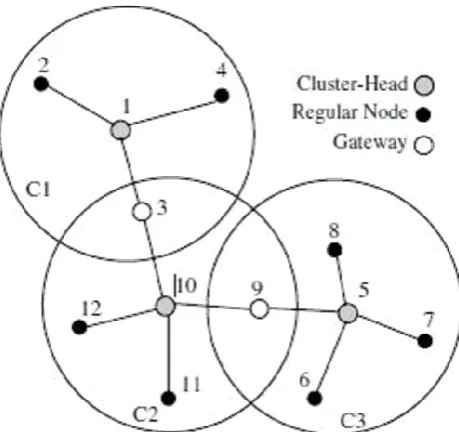
hierarchy (which is required in MMWN). Instead, each clu ster is maintained with a cluster-head, which is a mobile node elected to manage all the other nodes within the c luster (see Fig. 2). This node controls the transm ission medium and all inter-cluster communications occur through this node. The advantage of this protocol is that each node only maintains routes to its cluster-head, which means that routing overheads are lower compared to flooding routing information through all the network. However, the re are significant overheads associated with maintaining clusters. This is because each node needs to periodically broadcast its cluster member table and update its table based on the received updates.
Figure 2. Illustration of a typical cluster-b ased network.
2.9. Hierarchical state routing (HSR)
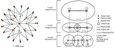
HSR [26] is also based on the traditional Link State algorithm. However, unlike the oth er link state based algorithm described so far, HSR maintains a hierar chical addressing and topology map. Clustering algorithm such as CGSR can be used to organise the nodes with close proximity into clusters. Each cluster has three types of nodes: a cluster-head node which acts as a local coordinator fo r each node, Gateway nodes which are nodes tha t lie in two different clusters, and internal nodes that are all the other n odes in each cluster. All nodes have a unique ID, which is typically the MAC address for each node. The nodes within each cluster broadcast their link information to each other. In HSR, each node also has a hierarchical ID (HID), which is a sequence of the MAC addresses from the top
hierarchy to the source node For example (see Fig. 3) the HID of no de 8 is 〈2,2,8〉. The HID can be used to send a packet from any source to any destination in the network. For exa mple, consider sending a packet from node 8 to node 3. Node 8 had a HID of〈2,2,8〉
and node 3 has a HID of 〈4,4,3〉. The packet is first sent to node 2 (top of h ierarchy). Node 2 then sends the packet to node 4, which is the top hierarchy of node 3. Node 2 and 4 form a “virtual link”, which is the path
〈2,9,5,6,4〉. Node 4 will then send th e packet to node 3. Logical clustering provides a logical relationship between the cluster-head at a higher level. Here, the nodes are assigned logical address of the form <subnet,host>. For example the logical node 2 in the level 2 of Fig. 3 has a logical address 〈2,2〉. The logical no des are connected via logical links, which form a “tunnel” between lower level clusters. Logical nodes exchange logical link information as well as a summary information of the lower leve l clusters. The logical link state information is then flooded down to the lower levels. The physical nodes at the lowest level will then have a “hierarchical” topology o f the network. The advantage of HSR over other hierarchical routing protocols (such as MMWN) is the separation of mobility management from the physical hierarchy. This is done via Hom e Agents. This protocol also has far less control overhead when compared t0 GSR and FSR. However, this protocol (similar to any other cluster based protocol) introduces extra overheads to the network from cluster formation and maintenance.
2.10. Optimised link state routing (OLSR)
which covers all of its two hop neighbours. For example, in Fig. 4, node A can select nodes B, C, K and N to be the MPR nodes. Since these nodes cover all the nodes, which are two hops away. Each node determines an optimal route (in terms of hops) to every known destination using its topology information (from the topology table and neighbouring table), and stores this information in a routing table. Therefore, routes to every destination are immediately available when data transmission begins.
Figure 3. Multipoint Relays.
2.11. Topology broadcast reverse path forwarding (TBRPF)
TBRPF [4] is another link-state based routing protocol, which performs hop-by-hop routing. The protocol uses the concept of reverse-path forwarding (RPF) to disseminate its update packets in the reverse direction along the spanning tree, which is made up of the minimum-hop path from the nodes leading to the source of the update message. In this routing strategy, each node calculates a source tree, which provides a path to all reachable destinations. This is done by applying a modified version of Dijkstra’s algorithm on the partial topology information stored in their topology table. In TBRPF, each node minimises overhead by reporting only part of their source tree to their neighbours. The reportable part of each source tree is exchanged with neighbouring nodes by periodic and differential hello messages. The differential hello messages only report the changes of the status of the neighbouring nodes. As a result, the hello messages in TBRPF are smaller than in protocols which report the complete link-state information.
2.12. Summary of proactive routing
In summary, most flat routed global routing protocols do not scale very well. This is because their updating procedure consumes a significant amount of network
bandwidth. From the flat routed protocols discussed in this section, OLSR may scale the best. This increase in scalability is achieved by reducing the number of rebroadcasting nodes through the use of multipoint relaying, which elects only a number of neighbouring nodes to rebroadcast the message. This clearly has the advantage of reducing, channel contention and the number of control packet travelling through the network when compared to strategies which use blind or pure flooding where all nodes rebroadcast the messages. The DREAM routing protocol also has scalability potential since it has significantly reduced the amount of overhead transmitted through the network, by exchanging location information rather than complete (or partial) link state information. The hierarchically routed global routing protocols will scale better most of the flat routed protocols, since they have introduced a structure to the network, which control the amount of overhead transmitted through the network. This is done by allowing only selected nodes such as a clusterhead can rebroadcast control information. The common disadvantage associated with all the hierarchical protocols is mobility management. Mobility management introduces unnecessary overhead to the network (such as extra processing overheads for cluster formation and maintenance).
3. Reactive routing protocols
On-demand routing protocols were designed to reduce the overheads in proactive protocols by maintaining information for active routes only. This means that routes are determined and maintained for nodes that require to send data to a particular destination. Route discovery usually occurs by flooding a route request packets through the network. When a node with a route to the destination (or the destination itself) is reached a route reply is sent back to the source node using link reversal if the route request has travelled through bi-directional links or by piggy-backing the route in a route reply packet via flooding. Therefore, the route discovery overhead (in the worst case scenario) willgrow by2 O(N+M) when link reversal is possible
means that the intermediate nodes do not need to maintain up-to-date routing information for each active route in order to forward the packet towards the destination. Furthermore, nodes do not need to maintain neighbour connectivity through periodic beaconing messages. The major drawback with source routing protocols is that in large networks they do not perform well. This is due to two main reasons; firstly as the number of intermediate nodes in each route grows, then so does the probability of route failure. To show this let P(f)=a·n, where P(f) is the probability of route failure, a is the probability of a link failure and n is the number of intermediate nodes in a route. From this,3 it
can be seen that as n→∞, then P(f)→∞. Secondly, as the number of intermediate nodes in each route grows, then the amount of overhead carried in each header of each data packet will grow as well. Therefore, in large networks with significant levels of multihoping and high levels of mobility, these protocols may not scale well. In hop-by-hop routing (also known as point-to-point routing) [8], each data packet only carries the destination address and the next hop address. Therefore, each intermediate node in the path to the destination uses its routing table to forward each data packet towards the destination. The advantage of this strategy is that routes are adaptable to the dynamically changing environment of MANETs, since each node can update its routing table when they receiver fresher topology information and hence forward the data packets over fresher and better routes. Using fresher routes also means that fewer route recalculations are required during data transmission. The disadvantage of this strategy is that each intermediate node must must store and maintain routing information for each active route and each node may require to be aware of their surrounding neighbours through the use of beaconing messages.A number of different reactive routing protocols have been proposed to increase the performance of reactive routing. This section describes a number of these strategies and makes a performance comparison between them.
3.1. Ad hoc on-demand distance vector (AODV)
The AODV [8] routing protocol is based on DSDV and DSR [19] algorithm. It uses the periodic beaconing and sequence numbering procedure of DSDV and a similar route discovery procedure as in DSR. However, there are two major differences between DSR and AODV. The most distinguishing difference is that in DSR each
packet carries full routing information, whereas in AODV the packets carry the destination address. This means that AODV has potentially less routing overheads than DSR. The other difference is that the route replies in DSR carry the address of every node along the route, whereas in AODV the route replies only carry the destination IP address and the sequence number. The advantage of AODV is that it is adaptable to highly dynamic networks. However, node may experience large delays during route construction, and link failure may initiate another route discovery, which introduces extra delays and consumes more bandwidth as the size of the network increases.
3.2. Dynamic source routing (DSR)
As stated earlier, the DSR protocol requires each packet to carry the full address (every hop in the route), from source to the destination. This means that the protocol will not be very effective in large networks, as the amount of overhead carried in the packet will continue to increase as the network diameter increases. Therefore in highly dynamic and large networks the overhead may consume most of the bandwidth. However, this protocol has a number of advantages over routing protocols such as AODV, LMR [7] and TORA [25], and in small to moderately size networks (perhaps up to a few hundred nodes), this protocol may perform better. An advantage of DSR is that nodes can store multiple routes in their route cache, which means that the source node can check its route cache for a valid route before initiating route discovery, and if a valid route is found there is no need for route discovery. This is very beneficial in network with low mobility. Since they routes stored in the route cache will be valid longer. Another advantage of DSR is that it does not require any periodic beaconing (or hello message exchanges), therefore nodes can enter sleep node to conserve their power. This also saves a considerable amount of bandwidth in the network.
3.3. Routing on-demand acyclic multi-path (ROAM)
multiple flood searches when the required destination is no longer reachable. Another advantage is that each router maintains entries (in a route table) for destinations, which flow data packets through them (i.e. the router is a node which completes/or connects a router to the destination). This reduces significant amount of storage space and bandwidth needed to maintain an up-to-date routing table. Another novelty of ROAM is that each time the distance of a router to a destination changes by more than a defined threshold, it broadcasts update messages to its neighbouring nodes, as described earlier. Although this has the benefit of increasing the network connectivity, in highly dynamic networks it may prevent nodes entering sleep mode to conserve power.
3.4. Light-weight mobile routing (LMR)
The LMR protocol is another on-demand routing protocol, which uses a flooding technique to determine its routes. The nodes in LMR maintain multiple routes to each required destination. This increases the reliability of the protocol by allowing nodes to select the next available route to a particular destination without initiating a route discovery procedure. Another advantage of this protocol is that each node only maintains routing information to their neighbours. This means avoids extra delays and storage overheads associated with maintaining complete routes. However, LMR may produce temporary invalid routes, which introduces extra delays in determining a correct loop.
3.5. Temporally ordered routing algorithm (TORA)
The TORA routing protocol is based on the LMR protocol. It uses similar link reversal and route repair procedure as in LMR, and also the creation of a DAGs, which is similar to the query/reply process used in LMR [30]. Therefore, it also has the same benefits as LMR. The advantage of TORA is that it has reduced the far-reaching control messages to a set of neighbouring nodes, where the topology change has occurred. Another advantage of TORA is that it also supports multicasting, however this is not incorporated into its basic operation. TORA can be used in conjunction with lightweight adaptive multicast algorithm (LAM) to provide multicasting. The disadvantage of TORA is that the algorithm may also produce temporary invalid routes as in LMR.
3.6. Associativity-based routing (ABR)
ABR [33] is another source initiated routing protocol, which also uses a query-reply technique to determine routes to the required destinations. However, in ABR route selection is primarily based on stability. To select stable route each node maintains an associativity tick with their neighbours, and the links with higher associativity tick are selected in preference to the once with lower associativity tick. However, although this may not lead to the shortest path to the destination, the routes tend to last longer. Therefore, fewer route reconstructions are needed, and more bandwidth will be available for data transmission. The disadvantage of ABR is that it requires periodic beaconing to determine thedegree of associativity of the links. This beaconing requirement requires all nodes to stay active at all time, which may result in additional power consumption. Another disadvantage is that it does not maintain multiple routes or a route cache, which means that alternate routes will not be immediately available, and a route discovery will be required using link failure. However, ABR has to some degree compensated for not having multiple routes by initiating a localised route discovery procedure (i.e. LBQ).
3.7. Signal stability adaptive (SSA)
SSA [9] is a descendent of ABR. However, SSA selects routes based on signal strength and location stability rather than using an associativity tick. As in ABR, the routes selected in SSA may not result in the shortest path to the destination. However, they tend to live longer, which means fewer route reconstructions are needed. One disadvantage of SSA when compared to DSR and AODV is that intermediate nodes cannot reply to route requests sent toward a destination, which may potentially create long delays before a route can be discovered. This is because the destination is responsible for selecting the route for data transfer. Another disadvantage of SSA is no attempt is made to repair routes at the point where the link failure occurs (i.e. such as an LBQ in ABR). In SSA the reconstruction occurs at the source. This may introduce extra delays, since the source must be notified of the broken like before another one can be found.
RDMR [1] attempts to minimise the routing overheads by calculating the distance between the source and the destination and therefore limiting each route request packet to certain number of hops (as described earlier). This means that the route discovery procedure can be confined to localised region (i.e. in will not have a global affect). RDMR also uses the same technique when link failures occurs (i.e. route maintenance). Thus conserving a significant amount of bandwidth and battery power. Another advantage of RDMR is that it does not require a location aided technology (such as a GPS) to determine the routing patterns. However, the relative-distance micro-discovery procedure can only be applied if the source and the destinations have communicated previously. If no previous communication record is available for a particular source and destination, then the protocol will behave in the same manner as the flooding algorithms (i.e. route discovery will have a global affect).
3.9. Location-aided routing (LAR)
LAR [21] is based on flooding algorithms (such as DSR). However, LAR attempts to reduce the routing overheads present in the traditional flooding algorithm by using location information. This protocol assumes that each node knows its location through a GPS. Two different LAR scheme were proposed in [21], the first scheme calculates a request zone which defines a boundary where the route request packets can travel to reach the required destination.The second method stores the coordinates of the destination in the route request packets. These packets can only travel in the direction where the relative distance to the destination becomes smaller as they travel from one hop to another. Both methods limit the control overhead transmitted through the network and hence conserve bandwidth. They will also determine the shortest path (in most cases) to the destination, since the route request packets travel away from the source and towards the destination. The disadvantage of this protocol is that each node is required to carry a GPS. Another disadvantage is (especially for the first method), that protocols may behave similar to flooding protocols (e.g. DSR and AODV) in highly mobile networks.
3.10. Ant-colony-based routing algorithm (ARA
ARA [13] attempt to reduce routing overheads by adopting the food searching behaviour of ants. When ants search for food they start from their nest and walk towards the food, while leaving behind a transient trail called pheromone. This indicated the path that has been taken by the ant and allows others to follow, until the pheromone disappears. Similar to AODV and DSR, ARA is also made up of two phases (route discovery and route maintenance). During route discovery a Forwarding ANT (FANT) is propagated through the network (similar to a RREQ). At each hop, each node calculate a pheromone value depending on how many number of hops the FANT has taken to reach them. The nodes then forward the FANT to their neighbours. Once the destination is reached, it creates a Backward ANT (BANT), and returns it to the source. When the source receives the BANT from the destination node, a path is determined and data packet dissemination begins. To maintain each route, each time a data packet travels between intermediate nodes the pheromone value is increased. Otherwise the pheromone value is decreased overtime until it expires. To repair a broken link, the nodes firstly check their routing table, if no route is found they inform their neighbours for an alternate route. If the neighbours do have a route they inform their neighbours by backtracking. If the source node is reached and no route is found, a new route discovery process is initiated. The advantage of this strategy is that the size of each FANT and BANT is small, which means the amount of overhead per control packet introduced in the network is minimised. However, the route discovery process it based on flooding, which means that the protocol may have scalability problems as the number of nodes and flows in the network grows.
3.11. Flow oriented routing protocol (FORP)
rebroadcasted. When a Flow_REQ packet reaches the destination, a Route Expiration Time (RET) is calculated using the minimum of all the LETs for each node in the route and a Flow_SETUP packet is sent Flow_HANDOFF message is generated and propagated via flooding (similar to a Flow_REQ). Flow_SETUp message along the newly chosen route. The advantage of this strategy compared to other on-demand routing protocols described so far is that it minimises the disruptions of real time sessions due to mobility by attempting to maintain constant flow of data. However, since it is based on pure flooding, the protocol may experience scalability problems in large networks.
3.12. Cluster-based routing protocol (CBRP)
Unlike the on-demand routing protocols described so far. In CBRP [17] the nodes are organised in a hierarchy. As most hierarchical protocols described in the previous section, the nodes in CBRP or grouped into clusters. Each cluster has a cluster-head, which coordinates the data transmission within the cluster and to other clusters. The advantage of CBRP is that only cluster heads exchange routing information, therefore the number of control overhead transmitted through the network is far less than the traditional flooding methods. However, as in any other hierarchical routing protocol, there are overheads associated with cluster formation and maintenance. The protocol also suffers from temporary routing loops. This is because some nodes may carry inconsistent topology information due to long propagation delay.
3.13. Summary of reactive routing
Generally, most on-demand routing protocols have the same routing cost when considering the worst-case
amount of processing overheads during cluster formation/maintenance. This protocol suffers from temporary invalid routes as the destination nodes travel from one cluster to another. Therefore, this protocol is suitable for medium size networks with slow to moderate mobility. The protocol may also best perform in scenarios with group mobility where the nodes within a cluster are more likely to stay together.
4. Hybrid routing protocols
Hybrid routing protocols are a new generation of protocol, which are both proactive and reactive in nature. These protocols are designed to increase scalability by allowing nodes with close proximity to work together to form some sort of a backbone to reduce the route discovery overheads. This is mostly
achieved by proactively maintaining routes to nearby nodes and determining routes to far away nodes using a route discovery strategy. Most hybrid protocols proposed to date are zone-based, which means that the network is partitioned or seen as a number of zones by each node. Others group nodes into trees or clusters. This section describes a number of different hybrid routing protocol proposed for MANETs. Furthermore, it provides a theoretical performance comparison between the described strategies. The discussion on the performance comparison is based on Table 5 and Table 6. Note that, Table 5 provides the summary of the characteristic feature of each strategy and Table 6 provides a theoretical performance evaluation. The performance metrics presented illustrates the worst case scenario for each routing protocol.
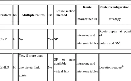
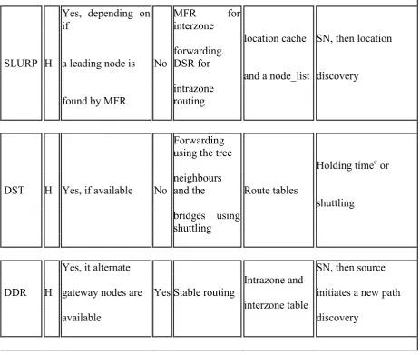
Table 5. Basic characteristics of hybrid routing protocols
Route
Route reconfiguration
Protocol
RS
Multiple routes
Bc
Route metric
method
maintained in
strategy
Intrazone and
Route repair at point
of
ZRP
F No
Yes SP
interzone tables failure and SN
aYes, if more than
SP or next
available
Intrazone and
ZHLS H one virtual link
No
Location request
bvirtual link
interzone tables
exists
Volume 2 | Issue 4 | July-August -2017 | www.ijsrcseit.com | UGC Approved Journal [ Journal No : 64718 ]
908
Yes, depending on
if
MFR
for
interzone
location cache SN, then location
SLURP H a leading node is
No
forwarding.
DSR for
and a node_list discovery
found by MFR
intrazone
routing
Forwarding
using the tree
Holding time
cor
DST
H Yes, if available
No
neighbours
and the
Route tables
shuttling
bridges using
shuttling
Yes, it alternate
SN, then source
Intrazone and
DDR
H gateway nodes are Yes Stable routing
initiates a new path
interzone table
available
discovery
RS=routing structure; H=hierarchical; F=flat; SP=shortest path; SN=source notification; Bc=beacons. a The source may or may not be notified.b A location request will be sent if the zone ID of a node changes c Packets are held for a short period of time during which the nodes attempts to route the packet directly to the destination.
Table 6. Complexity comparison of hybrid routing protocols
Protocol
TC[RD]
TC[RM]
CC[RD]
CC[RM]
Advantage
Disadvantage
Intra:
Reduce
Overlapping
ZRP
O(
I
)/Inter:
O(
I
)/O(2
D
) O(
Z
N)/O(
N
+
V
) O(
Z
N)/O(
N
+
V
)
retransmissions zones
O(2
D
)
Intra:
Reduction of
Static zone map
ZHLS
O(
I
)/O(
D
) O(
N
/
M
)/O(
N
+
V
) O(
N
/
M
)
a/O(
N
+
V
)
O(
I
)/Inter:
SPF, low CO
required
TC=time complexity; CC=communication complexity; RD=route discovery; RM=route maintenance;I=periodic update interval; N=number of nodes in the network; M=number of zones or cluster in the network;ZN=number of nodes in a zone, cluster or tree; ZD=diameter of a zone, cluster or tree; Y=number of nodes in the path to the home region; V=number of nodes on the route reply path; SPF=single point of failure; CO=control overhead.a In ZHLS, the intrazone is maintained proactively. Therefore, a fixed number of updates are sent at a fixed interval b In SLURP, in the worst-case scenario, the source node and the home region of the destination are on the opposite edges of the network.
4.1. Zone routing protocol (ZRP)
In ZRP [14], the nodes have a routing zone, which defines a range (in hops) that each node is required to maintain network connectivity proactively. Therefore,
for nodes within the routing zone, routes are immediately available. For nodes that lie outside the routing zone, routes are determined on-demand (i.e. reactively), and it can use any on-demand routing protocol to determine a route to the required destination. The advantage of this protocol is that it has significantly reduced the amount of communication overhead when compared to pure proactive protocols. It also has reduced the delays associated with pure reactive protocols such as DSR, by allowing routes to be discovered faster.This is because, to determine a route to a node outside the routing zone, the routing only has to travel to a node which lies on the boundaries (edge of the routing zone) of the required destination. Since the boundary node would proactively maintain routes to the destination (i.e. the boundary nodes can complete the route from the source to the destination by sending a reply back to the source with the required routing address). The disadvantage of ZRP is that for large values of routing zone the protocol can
Protocol
TC[RD]
TC[RM]
CC[RD]
CC[RM]
Advantage
Disadvantage
O(
D
)
Intra:
Location
Static
zone
map
SLURP O(2
Z
D)/Inter:
O(2
Z
D/O(2
D
)
O(2
)
N
/
M
)/O(2
Y
O(2
N
/
M
)/O(2
Y
) discovery using
required
O(2
D
)
bhome regions
Intra:
Reduce
DST
O(
Z
D)/Inter: O(
Z
D)/O(
D
) O(
Z
N)/O(
N
)
O(
Z
N)/O(
N
)
Root node
retransmissions
O(
D
)
Preferred
Intra:
No zone map
or
neighbours
may
DDR O(
I
)/Inter: O(
I
)/O(2
D
) O(
Z
N)/O(
N
+
V
) O(
Z
N)/O(
N
+
V
)
zone
coordinator
become
O(2
D
)
bottlenecks
behave like a pure proactive protocol, while for small values it behaves like a reactive protocol.
4.2. Zone-based hierarchical link state (ZHLS)
Unlike ZRP, ZHLS [18] routing protocol employs hierarchical structure. In ZHLS, the network is divided into non-overlapping zones, and each node has a node ID and a zone ID, which is calculated using a GPS. The hierarchical topology is made up of two levels: node level topology and zone level topology, as described previously. In ZHLS location management has been simplified. This is because no cluster-head or location manager is used to coordinate the data transmission. This means there is no processing overhead associated with cluster-head or Location Manager selection when compared to HSR, MMWN and CGSR protocols. This also means that a single point of failure and traffic bottlenecks can be avoided. Another advantage of ZHLS is that it has reduced the communication overheads when compared to pure reactive protocols such as DSR and AODV. In ZHLS, when a route to a remote destination is required (i.e. the destination is in another zone), the source node broadcast a zone-level location request to all other zones, which generates significantly lower overhead when compared to the flooding approach in reactive protocols. Another advantage of ZHLS is that the routing path is adaptable to the changing topology since only the node ID and the zone ID of the destination is required for routing. This means that no further location search is required as long as the destination does not migrate to another zone. However, in reactive protocols any intermediate link breakage would invalidate the route and may initiate another route discovery procedure. The Disadvantage of ZHLS is that all nodes must have a preprogrammed static zone map in order to function. This may not feasible in applications where the geographical boundary of the network is dynamic. Nevertheless, it is highly adaptable to dynamic topologies and it generates far less overhead than pure reactive protocols, which means that it may scale well to large networks.
4.3. Scalable location update routing protocol (SLURP)
Similar to ZLHS, in SLURP [34] the nodes are organised into a number of non-overlapping zones. However SLURP further reduces the cost of maintaining routing information by eliminating a
global route discovery. This is achieved by assigning a home region for each node in the network. The home region for each node is one specific zone (or region), which is determined using a static mapping function, f(NodeID)→regionID, where f is a many-to-one function that is static and known to all nodes. An example of a function that can perform the static zone mapping is f(NodeID)=g(NodeID)modK[34], where g(NodeID) is a random number generating function that uses the node ID as the seed and output a large number, and k is the total number of home regions in the network. Now since the node ID of each node is constant (i.e. a MAC address), then the function will always calculate the same home region. Therefore, all nodes can determine the home region for each node using this function provided they have their node ID. Each node maintains its current location (current zone) with the home region by unicasting a location update message towards its home region. Once the location update packet reaches the home region, it is broadcasted to all the nodes in the home region. Hence, to determine the current location of any node, each node can unicast a location_discovery packet to the required nodes home region (or the area surrounding the home region) in order to find its current location. Once the location is found, the source can start sending data towards the destination using the most forward with fixed radius (MFR) geographical forwarding algorithm. When a data packet reaches the region in which the destination lies, then source routing4 is used to get the data packet to the destination. The disadvantage of SLURP is that it also relies on a preprogrammed static zone map (as does ZHLS).
4.4. Distributed spanning trees based routing protocol (DST)
packet is held for a period of time called holding time. The idea behind the holding time is that as connectivity increases, and the network becomes more stable, it might be useful to buffer and route packets when the network connectivity is increased over time. In DST, the control packets are disseminated from the source are rebroadcasted along the tree edges. When a control reaches down to a leaf node, it is sent up the tree until it reaches a certain height referred to as the shuttling level. When the shuttling level is reached, the control packet can be sent down the tree or to the adjoining bridges. The main disadvantage of the DST algorithm is that it relies on a root node to configure the tree, which creates a single point of failure. Furthermore, the holding time used to buffer the packets may introduce extra delays in to the network.
4.5. Distributed dynamic routing (DDR)
DDR [24] is also a tree-based routing protocol. However, unlike DST, in DDR the trees do not require a root node. In this strategy tree are constructed using periodic beaconing messages which is exchanged by neighbouring nodes only. The trees in the network form a forest, which is connected together via gateway nodes (i.e. nodes which are in transmission range but belong to different trees). Each tree in the forest forms a zone which is assigned a zone ID by running a zone naming algorithm. Furthermore, since each node can only belong to a single zone (or tree), then the network can be also seen as a number of non-overlapping zones. The DDR algorithm consists of six phases: preferred neighbour election, forest construction, intra-tree clustering, inter-tree clustering, zone naming and zone partitioning. Each of these phases are executed based on information received in the beacon messages. During the initialisation phase, each node starts in the preferred neighbour election phase. The preferred neighbour of a node is a node that has the most number of neighbours. After this, a forest is constructed by connecting each node to their preferred neighbour. Next, the intra-tree clustering algorithm is initiated to determine the structure of the zone5 (or the tree) and to build up the intra-zone routing table. This is then followed by the execution of the inter-tree algorithm to determine the connectivity with the neighbouring zones. Each zone is then assigned a name by running the zone naming algorithm and the network is partitioned into a number of non-overlapping zones. To determine routes, hybrid ad hoc routing protocols (HARP) [23] to work
on top of DDR. HARP uses the intra-zone and inter-zone routing tables created by DDR to determine a stable path between the source and the destination. The advantage of DDR is that unlike ZHLS, it does not rely on a static zone map to perform routing and it does not require a root node or a clusterhead to coordinate data and control packet transmission between different nodes and zones. However, the nodes that have been selected as preferred neighbours may become performance bottlenecks. This is because they would transmit more routing and data packets than every other nodes. This means that these nodes would require more recharging as they will have less sleep time than other nodes. Furthermore, if a node is a preferred neighbour for many of its neighbours, many nodes may want to communicate with it. This means that channel contention would increase around the preferred neighbour, which would result in larger delays experienced by all neighbouring nodes before they can reserve the medium. In networks with high traffic, this may also result in significant reduction in throughput, due to packets being dropped when buffers become full.
III.
RESULTS AND DISCUSSION
Summary of Hybrid Routing
IV.CONCLUSION
In this paper three categories of unicast routing protocols (some have multicast capability) where introduced (Table 7). The global routing protocols, which are derived mainly from the traditional link state or distance vector algorithm, maintain network connectivity proactively, and the on-demand routing protocols determine routes when they are needed. The hybrid routing protocols employ both reactive and proactive properties by maintaining intra-zone information proactively and inter-zone information reactively. By looking at performance metrics and characteristics of all categories of routing protocols, a number of conclusions can be made for each category. In global routing flat addressing can be simple to implement, however it may not scale very well for large networks [15]. In order to make flat addressing more efficient, the number of routing overheads introduced in the networks must be reduced. One way to do this is to use a device such a GPS. For example, in the DREAM routing protocol, node only exchange location information (coordinates) rather than complete link state or distance vector information. Another way to reduce routing overheads is by using conditional updates rather than periodic ones. For example in the STAR routing protocol, updates occur based on three conditions (as described earlier). The global routing schemes, which use hierarchical addressing, have reduced the routing overheads introduced to the networks by introducing a structure, which localises the update message propagation. However, the current problem with these schemes is location management, which also introduces significant overheads to the network. In on-demand routing protocols, the flooding-based routing protocols such as DSR and AODV will also have scalability problems. In order to increase scalability, the route discovery and route maintenance must be controlled. This can be achieved by localising the control message propagation to a defined region where the destination exists or where the link has been broken. For example, in the LAR1 routing protocol, perform well in large networks. The advantage of these protocols over other hierarchical routing protocols is
that they have a simplified location management due to using a GPS and do not use a cluster-head to coordinate data transmission, which means that a single point of failure and performance bottlenecks can be avoided. Another advantage of these protocols is that they are highly adaptable to changing topology since only the node ID and zone ID of the destination is required for routing to occur. The ZRP routing protocol is another hybrid routing protocol described earlier, which is designed to increase the scalability of MANETs. The advantage of this protocol is that it maintains a strong network connectivity (proactively) within the routing zones while determining remote route (outside the routing zone) quicker than flooding. Another advantage of the ZRP is that it can incorporate other protocols to improve its performance.
V.
REFERENCES
[1]. G. Aggelou, R. Tafazolli, RDMAR: a bandwidth-efficient routing protocol for mobile ad hoc networks, in: ACM International Workshop on Wireless Mobile Multimedia (WoWMoM), 1999, pp. 26–33.
[2]. S. Basagni, I. Chlamtac, V.R. Syrotivk, B.A. Woodward, A distance effect algorithm for mobility (DREAM), in: Proceedings of the Fourth Annual ACM/IEEE International Conference on Mobile Computing and Networking (Mobicom’98), Dallas, TX, 1998. [3]. R.E. Bellman, Dynamic Programming, Princeton
University Press, Princeton, NJ (1957).
[4]. B. Bellur, R.G. Ogier, F.L Templin, Topology broadcast based on reverse-path forwarding routing protocol (tbrpf), in: Internet Draft, draft-ietf-manet-tbrpf-06.txt, work in progress, 2003. mobile wireless networks with fading channel, in: Proceedings of IEEE SICON, April 1997, pp. 197–211.
[7]. M. S. Corson, A. Ephremides, A distributed routing algorithm for mobile wireless networks, ACM/Baltzer Wireless Networks, 1 (1) (1995), pp. 61–81.
draft-ietf-manet-aodv-11.txt, work in progress, 2002.
[9]. R. Dube, C. Rais, K. Wang, S. Tripathi, Signal stability based adaptive routing (ssa) for ad hoc mobile networks, IEEE Personal Communication, 4 (1) (1997), pp. 36–45.
[10]. L. R. Ford, D.R. Fulkerson, Flows in Networks, Princeton University Press, Princeton, NJ (1962). [11]. J. J. Garcia-Luna-Aceves, C. Marcelo Spohn, Source-tree routing in wireless networks, in: Proceedings of the Seventh Annual International Conference on Network Protocols Toronto, Canada, October 1999, p. 273.
[12]. M. Gerla, Fisheye state routing protocol (FSR) for ad hoc networks, Internet Draft, draft-ietf-manet-aodv-03.txt, work in progress, 2002. [13]. M. Günes, U. Sorges, I. Bouazizi, Ara––the
ant-colony based routing algorithm for manets, in: ICPP workshop on Ad Hoc Networks (IWAHN 2002), August 2002, pp. 79–85.
[14]. Z. J. Hass, R. Pearlman, Zone routing protocol for ad-hoc networks, Internet Draft, draft-ietf-manet-zrp-02.txt, work in progress, 1999.
[15]. A. Iwata, C. Chiang, G. Pei, M. Gerla, T. Chen, Scalable routing strategies for multi-hop ad hoc wireless networks, IEEE Journal on Selected Areas in Communcations, 17 (8) (1999), pp. 1369–1379.
[16]. P. Jacquet, P. Muhlethaler, T. Clausen, A. Laouiti, A. Qayyum, L. Viennot, Optimized link state routing protocol for ad hoc networks, IEEE INMIC, Pakistan, 2001.
[17]. M. Jiang, J. Ji, Y.C. Tay, Cluster based routing protocol, Internet Draft, draft-ietf-manet-cbrp-spec-01.txt, work in progress, 1999.
[18]. M. Joa-Ng, I.-T. Lu, A peer-to-peer zone-based two-level link state routing for mobile ad hoc networks, IEEE Journal on Selected Areas in Communications, 17 (8) (1999), pp. 1415–1425. [19]. D. Johnson, D. Maltz, J. Jetcheva, The dynamic
source routing protocol for mobile ad hoc networks, Internet Draft, draft-ietf-manet-dsr-07.txt, work in progress, 2002.
[20]. K. K. Kasera, R. Ramanathan, A location management protocol for hierarchically organised multihop mobile wireless networks, in: Proceedings of the IEEE ICUPC’97, San Diego, CA, October 1997, pp. 158–162.
[21]. Y. B. Ko, N.H. Vaidya, Location-aided routing (LAR) in mobile ad hoc networks, in:
Proceedings of the Fourth Annual ACM/IEEE International Conference on Mobile Computing and Networking (Mobicom’98), Dallas, TX, 1998.
[22]. S. Murthy J.J. Garcia-Luna-Aceves, A routing protocol for packet radio networks, in: Proceedings of the First Annual ACM International Conference on Mobile Computing and Networking, Berkeley, CA, 1995, pp. 86– 95.
[23]. N. Nikaein, C. Bonnet, N. Nikaein, Harp-hybrid ad hoc routing protocol, in: Proceedings of IST: International Symposium on Telecommunications, September 1–3 Tehran, Iran, 2001.
[24]. N. Nikaein, H. Laboid, C. Bonnet, Distributed dynamic routing algorithm (ddr) for mobile ad hoc networks, in: Proceedings of the MobiHOC 2000: First Annual Workshop on Mobile Ad Hoc Networking and Computing, 2000.
[25]. V. D. Park, M.S. Corson, A highly adaptive distributed routing algorithm for mobile wireless networks, in: Proceedings of INFOCOM, April 1997.
[26]. G. Pei, M. Gerla, X. Hong, C. Chiang, A wireless hierarchical routing protocol with group mobility, in: Proceedings of Wireless Communications and Networking, New Orleans, 1999.
[27]. C. E. Perkins, T.J. Watson, Highly dynamic destination sequenced distance vector routing (DSDV) for mobile computers, in: ACM SIGCOMM’94 Conference on Communications Architectures, London, UK, 1994.
[28]. S. Radhakrishnan, N.S.V Rao, G. Racherla, C.N. Sekharan, S.G. Batsell, DST––A routing protocol for ad hoc networks using distributed spanning trees, in: IEEE Wireless Communications and Networking Conference, New Orleans, 1999. [29]. J. Raju, J. Garcia-Luna-Aceves, A new approach
to on-demand loop-free multipath routing, in: Proceedings of the 8th Annual IEEE International Conference on Computer Communications and Networks (ICCCN), Boston, MA, October 1999, pp. 522–527.
[31]. A. Udaya Shankar, C. Alaettinoglu, I. Matta, K. Dussa-Zieger, Performance comparison of routing protocols using MaRS: distance-vector versus link-state, in: Proceedings of the 1992 ACM SIGMETRICS and PERFORMANCE ’92 Int’l. Conf. on Measurement and Modeling of Computer Systems, Newport, RI, USA, 1–5 June 1992, p. 181.
[32]. W. Su, M. Gerla, Ipv6 flow handoff in ad-hoc wireless networks using mobility prediction, in: IEEE Global Communications Conference, Rio de Janeiro, Brazil, December 1999, pp. 271–275. [33]. C. Toh, A novel distributed routing protocol to
support ad-hoc mobile computing, in: IEEE 15th Annual International Phoenix Conf., 1996, pp. 480–486.