The prediction of chemosensory effects of volatile organic compounds in humans

(1)

Th e Pr e d ic t io n o f Ch e m o s e n s o r y Ef f e c t s o f Vo l a t il e Or g a n ic Co m p o u n d s in Hu m a n s

A Thesis presented to the University of London in partial fulfilment of the requirements for the degree of Doctor of Philosophy in the Faculty of Science

by

Joëlle Muriel Rachel Gola

Sir Christopher Ingold Laboratory Chemistry Department

(2)

ProQuest Number: U 643957

INFORMATION TO ALL USERS

The quality of this reproduction is dependent upon the quality of the copy submitted.

In the unlikely event that the author did not send a complete manuscript

and there are missing pages, th ese will be noted. Also, if material had to be removed, a note will indicate the deletion.

uest.

ProQuest U 643957

Published by ProQuest LLC(2016). Copyright of the Dissertation is held by the Author.

This work is protected against unauthorized copying under Title 17, United States Code. Microform Edition © ProQuest LLC.

ProQuest LLC

789 East Eisenhower Parkway P.O. Box 1346

(3)

(4)

ABSTRACT

An introduction to indoor air pollution is given, and the chemosensory effects in humans of volatile organic compounds (VOCs), singly and in binary mixtures, are

described, together with the bioassays already developed to quantify the effects of VOCs. The need for predictive models that can take over the bioassays is emphasised.

Attention is drawn to the establishment of mathematical models to predict the chemosensory effects of VOCs in humans. Nasal pungency threshold (NPT), eye irritation threshold (EIT) and odour detection threshold (ODT) values are available for a series of VOCs that cover a large range of solute properties. Each of these sets of

biological data are regressed against the corresponding solute descriptors, E, S, A, B and L to obtain quantitative structure activity relationships (QSARs) for log(l/NPT), log(l/ODT) and log(l/EIT) taking on the form:

LogSP = c + e.E + s.S + a.A + b.B + l.L

The availability of solute descriptors is investigated. It is shown that solute descriptors, E an excess molar refraction, S the solute dipolarity/polarizability, A the

solute overall hydrogen-bond acidity, B the solute overall hydrogen-bond basicity and L the logarithmic value of the solute Ostwald solubility coefficient in hexadecane at 298K, can be obtained through the use of various thermodynamic measurements. In this way descriptors for some 300 solutes have been obtained.

A headspace gas chromatographic method is also devised to determine the 1:1

complexation constant, K, between hydrogen bond donors and hydrogen bond acceptors

in octan-l-ol. The 30 complexation constants measured are then correlated with «2^ * a combination of the solute 1:1 hydrogen bond acidity and basicity, respectively, to

give:

(5)

List of Tables

Table 1.1. Sources of Volatile Organic Compounds, excluding methane, in the 3 outdoor air of United Kingdom in 1995

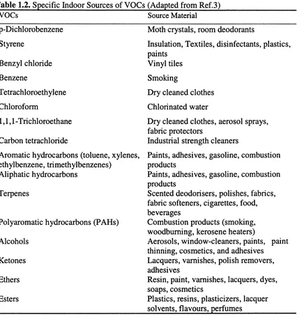
Table 1.2. Specific Indoor Sources of Volatile Organic Compounds 5

Table 1.3. Summary of Indoor Air and Outdoor Air Concentrations and Exposures 10 Table 1.4. Concentration of Volatile Organic Compounds in Indoor Air and 11

Outdoor Air in Avon, England

Table 1.5. Average Concentration of Indoor and Outdoor Air Pollutant in Offices 12

Table 1.6. Health Effects of Selected Volatile Organic Compounds 17

Table 1.7. Indoor Sources for Formaldehyde Exposure 17

Table 1.8. Effects of Formaldehyde on Humans after Short-term Exposure 18 Table 1.9. Typical Concentration of Indoor Volatile Organic Compounds Compared 19

to Threshold Limit Values

Table 2.1. Comparison of the receptor Codes for Odorants that have Similar 34 Structures but Different Odors

Table 2.2. Model for Odor Detection Thresholds Proposed by Hau and Connel 53 Table 2.3. Model for Nasal Pungency Thresholds Proposed by Hau and Connel 55

Table 3.1. Atom Contributions for Calculation of Vx 72

Table 3.2. Comparison Between «2” and descriptors 75

Table 3.3. Comparison between P2** and Z^2^ descriptors 76

Table 3.4. Water / Solvent and Gas / Solvent Processes used in the Determination of 79 Solute Descriptors

Table 3.5. Availability of Solute Descriptors 79

Table 3.6. Old and New Notation of the Abraham Solute Descriptors 83

Table 3.7. Output of the Regression Analysis Output of logP^^ and Solute 89 Descriptors

Table 4.1. System Constants for non-ionic Stationary Phases (395-397K) 113

Table 6.1. Estimation of log Vq at 298K 124

Table 6.2. Calculation of log from UI298 values 124

Table 6.3. Determination for log values from Solubility Data 125

Table 6.4. Test Set of Compounds 128

Table 6.5. Output of the Regression Analysis Output of log and Solute 130 Descriptors

(13)

Table 6.7. Table 6.8. Table 6.9. Table 6.10. Table 6.11. Table 7.1. Table 7.2. Table 7.3. Table 7.4. Table 7.5. Table 7.6. Table 7.7. Table 7.8. Table 7.9. Table 7.10. Table 7.11. Table 8.1. Table 8.2. Table 8.3. Table 8.4. Table 8.5. Table 8.6. Table 8.7. Table 8.8. 135 137 151 155 162 163 Descriptors

Water / Alkane and Gas / Alkane partition Processes at 298K System Constants for Squalane and Apolane

Observed Retention Index and Partition Coefficient Values together with 141 Calculated Partition Coefficient values for Gas / Squalane and Water / Squalane Systems at 298K

Data for Gas / Apolane Partition Process at 313K Estimation of L values from log and E values List of Refrigerants

Values of A used in equation (7.4)

Gas / Solvent and Water / Solvent Partition Coefficients Calculated from 165 Henry’s Law Coefficients

Regression Coefficients in equation (7.1) for Partition from Water at 166 298K

Regression Coefficients in equation (7.2) for Partition from the Gas 167 Phase at 298K

List of 0 values 168

Comparison between Observed and Calculated Partition Measurements 172 after ’Solver analysis’ for R23

Descriptors of the Refrigerants Calculated A and CTi values Observed and Calculated E values

Squared Dipole Moment and S values for halogenated n-alkanes used in 183 equation (7.9)

System Constant for Various Mixtures of Methanol in Water on a C-18 195 Stationary Phase

Ratio Coefficients for Griffin et al. data set 195

The Dependent Variables for Processes in Tables 8.1, 8.8 and 8.12 for a- 198 Terpineol; calculation of descriptors

Descriptors for terpenes from HPLC and GLC data 199

Calculation of Solvation descriptors by the method of ‘leave-one-out’ for 201 a-terpineol

Observed and Calculated values for B for terpenes using the structural 205 constants in Table 8.13

Name and Composition of Stationary phases 207

Solvation equations for GLC processes 209

(14)

Table 8.9. Table 8.10. Table 8.11. Table 8.12. Table 8.13. Table 8.14. Table 9.1. Table 9.2. Table 9.3. Table 9.4. Table 9.5. Table 9.6. Table 10.1. Table 10.2. Table 10.3. Table 10.4. Table 10.5. Table 11.1. Table 11.2. Table 12.1. Table 12.2. Table 123. Table 12.4. Table 12.5. Table 12.6.

The Dependent Variables for Processes in Table 8.6 for a-copaene; 213 calculation of descriptors

Solvation Descriptors for Terpenes 214

Experimental HPLC capacity factors measured by Griffin et al 217

System Constants for Various Processes at 298K 218

Calculated and Experimental Descriptors for a series of terpenes 219 Values of sB for functional groups, used to calculate descriptors for 220 terpenes

Output of the regression analysis of log (1/NPT) and Solute descriptors 232 Observed log (NPT) values, NPT in ppm, and log (NPT) values 236 calculated on equations (9.1) and (9.3)

Statistical results 236

NPT values (in ppm) measured via glass vessel experiments 238 Descriptors for 51 VOCs, observed log (1/NPT) and calculated log 240 (1/NPT) on equations (9.2) and (9.4). NPT values measured via squeeze bottle experiments

Solvation equations for gas / solvent partition processes 241 Regression coefficients in equations (10.2) for gas / solvent (phase) 250 partitions at 298K

Equations developed in the present work 258

Comparison of complexation of VOCs with porcine GBPs and odor 259 thresholds

Values of log (1/ODT) with ODT in ppm and VOC descriptors used in 263 the present work

Descriptors for higher homologous 264

Estimation of Chemosensory potency of the refrigerants 272 Selection of VOCs with descriptors and predictive chemosensory effects 276 on Humans

Values of constants m and c for various solvents 283

Empirical solvent parameters for selected solvents 286

Relationship between the slope, m, and various empirical polarity 290 parameters

Relationship between the intercept, c, and various empirical polarity 290 parameters

Calculated values of the slope m and intercept c for a series of solvents 291

(15)

Table 12.7. Log L values for butan-l-ol and heptan-2-one 293 Table 12.8. Maximum concentration, in mol.dm-3, at the chemosensory receptor area 293

for butan-l-ol and heptan-2-one taking dimethylformamide and octan-l- ol

Table 12.9. Determination of the amount reacted and the percentage of interaction 294 between butan-l-ol and heptan-2-one at the receptor area

Table 12.10. List of hydrogen bond acids and bases used in the present work 302

Table 12.11. Gas chromatographic conditions 301

Table 12.12. Retention times for a series of alkanes 304

Table 12.13. Kn and r^ values 311

Table 12.14. Validation of experimental method by comparing observed logK values 314 in n-hexadecane with calculated log K values in cyclohexane

Table 12.15. Headspace analysis results in n-hexadecane solvent 318

Table 12.16. Initial concentration in pentan-l-ol and in decane in n-hexadecane and 319 ratio of peak area values

Table 12.17. Headspace analysis results in octan-l-ol solvents 320

(16)

List of Figures

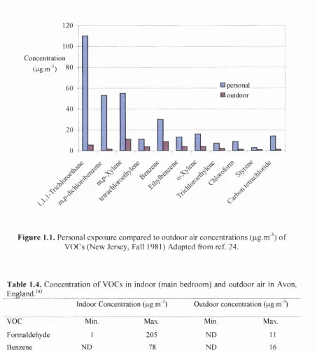
Figure 1.1. Personal exposure compared to outdoor air concentrations of VOCs 11 Figure 2.1. Key Organs thought to be involved in the perception of odor 27 Figure 2.2. Convergence of receptor cells signals on to glomeruli on the olfactory

bulb

27

Figure 2.3. Schematic representation of a putative odorant receptor 29

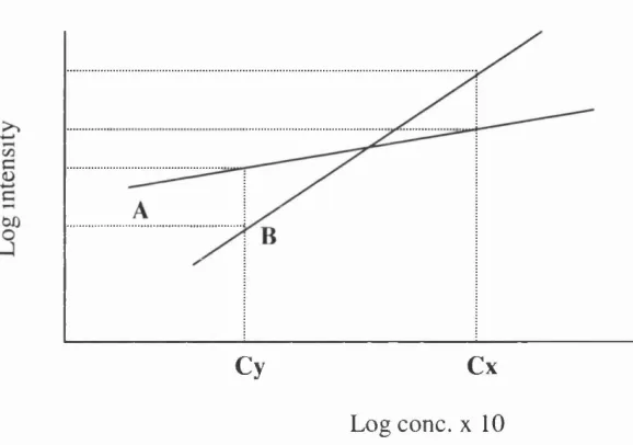
Figure 2.4. Perceived intensity vs log perfume concentration for two odorants 37 Figure 2.5. Monorhinic nasal testing via pop-up spout on the cap of the squeeze

bottle

43

Figure 2.6. Olfactory mechanism according to Hau and Connell 53

Figure 3.1. The three steps of the cavity model solvation 65

Figure 4.1. Process of chromatography 95

Figure 4.2. Example of chromatogram 98

Figure 4.3. Principle of static headspace gas chromatography 107

Figure 4.4. Equilibrium between the gas phase and the liquid phase 108

Figure 4.5. Components D and A in equilibrium between the gas and the liquid 109 phase

Figure 4.6. Structure of the phase HIO 112

Figure 6.1. Distribution of the descriptor E 127

Figure 6.2. Distribution of the descriptor L 127

Figure 6.3. Distribution of the dependent variable log 127

Figure 6.4. Plot of observed against calculated on equation (6.18) 129

Figure 6.5. Plot of observed against calculated log P^^ on equation (6.21) 132 Figure 6.6. Plot of e-coefficient values against the temperature, T (K) 138 Figure 6.7. Plot of 1-coefficient values against the temperature, T (K) 138

Figure 7.1. Plot of sd (P+L) against A 171

Figure 7.2. Plot of observed versus calculated E values for the test set of 175 compounds

Figure 8.1. Biological formation of terpenes 187

Figure 8.2. Structure, isoprene units and original chain of three important terpenes 188

Figure 8.3. The eight diastereoisomers of Menthol 189

Figure 8.4. Backbone structure 192

Figure 8.5. Relative regression against the percentage of methanol 196

(17)

Figure 8.7. Distribution of 0 values according to the phase properties 211 Figure 9.1. Plot of observed values of log (1/NPT) against log (1/NPT) calculated 233

on equation (9.2)

Figure 9.2. Plot of observed values of log (1/NPT) against log (1/NPT) calculated 233 on equation (9.4)

Figure 9.3. Principal component scores plot 235

Figure 9.4. Plot of observed values of log (1/NPT) against log (1/NPT) calculated 239 on equation (9.4)-comparison between two methods of measurements Figure 9.5. Plot of observed values of log (1/NPT) against log (1/NPT) calculated 239

on equation (9.5)-comparison between two methods of measurements

Figure 10.1. A possible model for odor thresholds 245

Figure 10.2. Plot of observed log (1/ODT) values against observed log (1/NPT) 248 values

Figure 10.3. Frequency of distribution of the descriptor L and for the variable log 249 (1/ODT)

Figure 10.4. Plot of observed log (1/ODT) against calculated values on equation 249 (10.4)

Figure 10.5. Plot of the residuals against the descriptor L. Figure 10.6. Residuals against the VOC maximum length

Figure 10.7. Example of maximum length determination, D, for pentan-2-one after 252 geometry optimisation

Figure 10.8. Plot of observed log (1/ODT) against log (1/ODT) on equation (10.8) 254 Figure 10.9. Plot of observed values of log (1/ODT) against calculated log (1/ODT) 256

on equation (10.9)

Figure 10.10. Plot of observed values of log (1/ODT) against calculated log (1/ODT) 256 on equation (10.10)

Figure 10.11. Plot of observed values of log (1/ODT) against the VOC maximum 260 length, for the homologous series of alkyl benzenes

Figure 10.12. Plot of observed values of log (1/ODT) against the VOC maximum 261 length, for the homologous series of acetates

Figure 11.1. Nasal pungency scale for selected VOCs 273

Figure 11.2. Eye irritation scale for selected VOCs Eye irritation scale for selected 274 VOCs

Figure 11.3. Odor detection scale for selected VOCs Figure 12.1. Hydrogen bond interaction between VOCs

Figure 12.2. Plot of log K^i values against «2" Pz" in selected solvents

251 251

(18)

Figure 8.7. Distribution of 0 values according to the phase properties 211 Figure 9.1. Plot of observed values of log (1/NPT) against log (1/NPT) calculated 233

on equation (9.2)

Figure 9.2. Plot of observed values of log (1/NPT) against log (1/NPT) calculated 233 on equation (9.4)

Figure 9.3. Principal component scores plot 235

Figure 9.4. Plot of observed values of log (1/NPT) against log (1/NPT) calculated 239 on equation (9.4)-comparison between two methods of measurements Figure 9.5. Plot of observed values of log (1/NPT) against log (1/NPT) calculated 239

on equation (9.5)-comparison between two methods of measurements

Figure 10.1. A possible model for odor thresholds 245

Figure 10.2. Plot of observed log (1/ODT) values against observed log (1/NPT) 248 values

Figure 10.3. Frequency of distribution of the descriptor L and for the variable log 249 (1/ODT)

Figure 10.4. Plot of observed log (1/ODT) against calculated values on equation 249 (10.4)

Figure 10.5. Plot of the residuals against the descriptor L. Figure 10.6. Residuals against the VOC maximum length

Figure 10.7. Example of maximum length determination, D, for pentan-2-one after 252 geometry optimisation

Figure 10.8. Plot of observed log (1/ODT) against log (1/ODT) on equation (10.8) 254 Figure 10.9. Plot of observed values of log (1/ODT) against calculated log (1/ODT) 256

on equation (10.9)

Figure 10.10. Plot of observed values of log (1/ODT) against calculated log (1/ODT) 256 on equation (10.10)

Figure 10.11. Plot of observed values of log (1/ODT) against the VOC maximum 260 length, for the homologous series of alkyl benzenes

Figure 10.12. Plot of observed values of log (1/ODT) against the VOC maximum 261 length, for the homologous series of acetates

Figure 11.1. Nasal pungency scale for selected VOCs 273

Figure 11.2. Eye irritation scale for selected VOCs Eye irritation scale for selected 274 VOCs

Figure 11.3. Odor detection scale for selected VOCs Figure 12.1. Hydrogen bond interaction between VOCs

Figure 12.2. Plot of log Ki;i values against in selected solvents

251 251

(19)

Figure 12.3. The system before and after addition of the component B 296 Figure 12.4. Schematic of gas chromatograms of the species A and D before and 297

after addition of B

Figure 12.5. Plot of ratio of peak area against the concentration for FEOH in octan- 305 l-ol

Figure 12.6. Plot of ratio of observed peak areas against ratio of concentration 309 Figure 12.7. Validation of experimental method by comparing observed log K 313

values in n-hexadecane with calculated log K values in cyclohexane

Figure 12.8. Plot of log Km for twenty-nine binary mixtures against the term of 315

0(2" Pi" for various acids and bases in octan-l-ol.

(20)

Acknowledgements

My sincere thanks go to Dr Michael Abraham for his help over the last three years of this project. His knowledge and expertise in the area of physical chemistry has

helped me to accomplish my Ph.D. I am extremely grateful for his unfailing encouragement, patience and guidance.

I would like to offer a particularly big thank you to my research group, Dr

Caroline Green, Dr Joelle Le, Dr Juliette Osei-Owusu, Dr Andrea Zissimos, Dr Jamie Platts; Kei Enomoto, Rui Figueira, Vikas Gupta, who have provided me with encouragement and great friendship over the years. Thanks also to Helene Field, who carried out some of the chromatographic measurements. Finally, I would like to wish Kei and Rui good luck in the completion of their own research.

I extend my gratitude to Dr J. Enrique Cometto-Muniz and Dr William Cain for all the chemosensory threshold values included in this work, and for providing me with their expertise and advice on various issues.

My thanks go to the Center for Indoor Airborne Research, CIAR - San Diego, California - for the funding of this project and giving me the opportunity to study for this PhD.

In addition, I would like to thank all those in the chemistry department who have

helped me in any way with my work or in making my time spent at University College London a happy one. In particular, Dimitra Georgeanopoulou, Camilla Forssten, and Paul Free for their tireless understanding and for always being here when I needed them. Thank you!

Thank you to all my friends in Gaillac, Toulouse, Paris and Cologne... Sophie I

wish you good luck in the completion of your thesis.

Importantly, I would like to thank my family for putting up with me during this PhD. My parents, to whom this thesis is dedicated, have shown never-ending encouragement, love and support. I would not have got so far without it. A big thank

you also to my sisters, Fabienne and Anne, and my two lovely nieces, Tatiana and Alexia for their love. This thesis is for you too! Finally, I would like to thank my grandma for her tireless support and love.

(21)

Chapter 1 An Introduction to Indoor Air Pollution

1.0. Introduction

For many individuals, the perception of risks from outdoor air is substantially higher than for indoor air, although the home environment is rarely considered to be a risk in this regard. However, exposure to indoor air pollutants (lAP) is a potentially serious public health problem in a wide variety of non industrial settings, for example,

residences, offices, schools and vehicles.^ Studies from the United States and Europe

show that persons in industrialised nations spend 90% or more of their time indoors.^

Infants, elderly, and those with pre-existing respiratory diseases are virtually inside all the time. As exposure to air pollution is a function of both time and concentration, the significance of the indoor environment for the total exposure of a person to a pollutant

can be high because of the time periods involved.^

While a good deal of public interest and concern continue to be directed at the effects of outdoor air pollution, notably traffic pollution, there is a growing tide of scientific studies that devotes sufficient attention to the indoor air environment. The understanding of the impact of indoor air pollution on human beings is of prime

necessity to improve indoor air quality and, then to reduce the number of illnesses and

discomfort.^ Over the recent years, a large number of projects have been designed to

gather information about the magnitude, extent, and causes of human exposure to indoor

air p o llu ta n ts .G u id e lin e s and standard levels have been proposed in an attempt to

reduce exposure to lAPs."^ Currently indoor air pollution is ranked by the United States

Environmental Protection Agency (US EPA) and the Centres for Disease Control and

Prevention in the top five environmental risks.^

(22)

air are formaldehyde, white spirit, and polyaromatic hydrocarbons, respectively. Furthermore, according to a definition given by the European Communities the expression "volatile organic compounds" means any compound having at 293.15 K a

vapour pressure of 0.01 kPa or more, or having a corresponding volatility under the particular condition of use.^ Next, VOCs contribute to a broad scale of chemicals with

production levels all over the world and widespread applications in industry, trade and private households. One of the most important industrial uses of the VOCs is their supply as solvents. In Table 1.1, sources and tonnage of VOCs found in air of the United Kingdom, in 1995, are displayed. The number of identified VOCs present in ambient air has risen steadily in recent years, from 250 to more than 900 in 1989, to

well more than 1,000 currently.^ Finally, the concentrations of VOCs are typically found to be substantially higher indoors than outdoors. Because we spend the vast majority of our time indoor, the prolonged exposure to high concentrations of VOCs is all too common.^ VOCs have been of increasing concern since the 1970s because of their potential to cause health effects similar to those reported in the Sick Building Syndrome and to contribute to respiratory problems and other diseases including cancer.^

The first section of this chapter deals with the various sources of air pollutants found indoors. The next section reports succinctly on the methods commonly used to assess exposure to indoor pollutant. Consequently, typical levels of indoor air pollutants are presented. Next, attention is drawn to the major health effects encountered by building occupants; effects due to exposure to VOCs are emphasised. The final section

discussed the various methods put forward to control indoor air pollutant levels.

1.1. Sources of Indoor Air Pollutant

Indoor air has been shown to be a complex mixture of chemical, biological and

physical ag en ts.A ctu ally , this complexity can be illustrated by the fact that some 4000

various components have been identified in tobacco smoke alone. Some of the most

important lAPs currently recognised are aeroallergen (cat allergen, house dust allergen...), micro-organisms (bacteria, fungi, fungal spores...), dust and particles

(23)

There are many sources of indoor air pollution at home. These include

combustion sources, such as oil, gas, kerosene, coal, wood, and tobacco products (e.g. benzene), a wide variety of building materials (e.g. toluene, xylenes, decane), cleaners, office products and machines, paints, and furnishings. Further, bathing (e.g. chloroform from hot water), cooking, cosmetics, hygienic products, plants, as well as human

biological processes give rise to lAP.^^ Table 1.2 gives examples of sources of VOCs known to be emitted indoor but this is far from comprehensive. Outdoor air may also contribute to indoor air contamination, particularly when air intakes are positioned near

parking areas, roads, or other locations where contaminated air may be entrained into the buildings. For example, car exhaust gases and particles can infiltrate into the home, especially if windows are opened.^

Source category Estimated Emissions

(thousand of tonnes) % Total

Power station 5

-Domestic 30 1.3

Commercial/Public service 2

-Refineries 2

-Iron and Steel 4

-Other Industrial Combustion 9 0.4

Non-Combustion Sources 335 14.3

Extraction and distillation of fossil fuel 334 14.3

Solvent use 700 29.9

Road Transport 690 29.5

Off road Sources 96 4.1

Military I

-Railways 8 0.3

Civil Aircraft 4

-Shipping 12 0.5

Waste treatment 26 1.1

Forest 80 3.4

Total 2338 100

Adapted from ref. 3.

Environmental tobacco smoke (ETS) is a source of particular concern because of the nuisance and irritation it can cause to users of multi-occupied buildings and the risks of disease to those inadvertently exposed to smoke. The main VOCs to be released in

sidestream smoke in quantities exceeding 1 mg per cigarette are nicotine, acetaldehyde,

(24)

and this has caused difficulties in apportioning the contribution that ETS makes to concentrations of particular pollutants within buildings.^

Three fundamental processes control the rate of VOC emissions from building sources: (1) evaporation; (2) desorption of absorbed compounds and (3) diffusion within a material. How fast the VOCs are produced depends on the process and the source

characteristics. The sources can be divided into those with continuous emissions, and

discontinuous emissions.^’ Firstly, some sources, such as building materials and

furnishings release pollutants more or less continuously. A process known as the ‘Sink Effect’, which is the absorption and desorption interactions between VOCs emitted and

the interior sources, also prolongs the presence of pollutant in the air.^^ For instance, a

forty-one day simulated chamber study indicated that an established material had absorbed about thirty VOCs, which were re-emitted to the chamber during the first

thirty days of the study.^^ Only thirteen of the VOCs originally present in the first days

of the study continued to be emitted in the final days, indicating that these thirteen were the only true components of the materials. Secondly, other sources, related to human activities carried out in the home, e.g. the use of solvents in cleaning, the use of pesticides in house keeping, release pollutants intermittently. The nature of emission and the variability of indoor spaces and ventilation conditions result in a dynamic

behaviour of air pollutants in indoor environment.^^

1.2. Assessm ent of Exposure

Assessment of exposure in humans refers to the analysis of various processes

that lead to human contact with pollutants after release in the environment.^^ The term exposure refers to the length of contact with the pollutant during a specified period of time. Assessment of exposure is a science on its own. It is not the purpose of this chapter to present the various processes involved in exposure assessment. Here,

attention is mainly drawn on methods used to determine pollutant concentration in indoor environments. Personal monitoring and biological monitoring are also defined.

The issue of exposure assessment has been recently reviewed recently by Wallace^"^ and

(25)

Table 1.2. Specific Indoor Sources of VOCs (Adapted from Ref.3)

VOCs Source Material

p-Dichlorobenzene Moth crystals, room deodorants

Styrene Insulation, Textiles, disinfectants, plastics,

paints

Benzyl chloride Vinyl tiles

Benzene Smoking

Tetrachloroethylene Dry cleaned clothes

Chloroform Chlorinated water

1,1,1 -Tiichloroethane Dry cleaned clothes, aerosol sprays, fabric protectors

Carbon tetrachloride Industrial strength cleaners

Aromatic hydrocarbons (toluene, xylenes. Paints, adhesives, gasoline, combustion ethylbenzene, trimethylbenzenes) products

Aliphatic hydrocarbons Paints, adhesives, gasoline, combustion

products

Terpenes Scented deodorisers, polishes, fabrics,

fabric softeners, cigarettes, food, beverages

Polyaromatic hydrocarbons (PAHs) Combustion products (smoking, woodbuming, kerosene heaters)

Alcohols Aerosols, window-cleaners, paints, paint

thinning, cosmetics, and adhesives

Ketones Lacquers, varnishes, polish removers,

adhesives

Ethers Resin, paint, varnishes, lacquers, dyes,

soaps, cosmetics

Esters Plastics, resins, plasticizers, lacquer

solvents, flavours, perfumes

1.2.1. M easu rem en t o f Volatile Organic C om pounds in Indoor Air

A wide range of sampling and analytical methods has been applied to determine

the nature and concentration of VOCs.^’^"^'^^ The most common methods are based on

collection using absorbents, e.g. Tenax TA, contained in a sampling tube or badge. The absorbent can be thermally desorbed and the VOCs can be determined by gas chromatography coupled with various detection systems. Other absorbents are available

(26)

the exposure period of the passive sampler is typically between one to four weeks

whereas for active sampling this can be achieved with sampling times of one hour. Other sampling methods are grab sampling, condensation, or liquid or solid-phase extraction. Solid-phase or liquid extraction is commonly used for less volatile compounds. A modified solid-phase extraction technique was put forward by PawU^^^^K,

and C O -w o r k e r s . T h e solid-phase microextraction technique (SPME) has now found a

number of applications in environmental fate s t u d i e s . M o r e recently, Elke and co-

workers^^ proposed an improved SPME technique to analyse benzene, toluene,

ethylbenzene and xylene (BTEX) in indoor air. Wallace has published a comprehensive

review gathering methods available to sample and analyse lAPs.^^ In 1999, Clement et

al. reviewed the latest techniques developed to examine lAPs.^^ Theory behind air

sampling and analysis is explained in a book.^^

Discomfort experienced in poor indoor air quality environment, is caused by simultaneous presence of individuals and air pollutants or in other words, individual’s exposure to air pollutants. The individual or personal exposure level is best assessed by measuring an individual’s contact with pollutants using personal monitoring or biological monitoring?^

1.2.2. P ersonal Monitoring

Measurements from personal monitoring indicate the level of external

exposure?"^ They are carried out by means of small devices, which sample lAPs, placed

on the individuals. For instance, bubblers, vapour adsorption tubes and passive samplers are widely used in personal monitoring to measure the concentration of airborne volatile

chemical in the region of the mouth.^^ These measurements can be carried out in real

environment or in simulated exposure chamber as explained later.

1.2.3. Biological Monitoring

According to the International Union of Pure and Applied Chemistry^^

(27)

compared to appropriate reference’. In other words, BM allows one to assess the integrated exposure by different routes, including ingestion, inhalation, dermal

absorption, blood, exhaled air and urine. Biological marker or biomarkers for exposure is an endogeneous substance or its metabolite or the product of interaction between a xenobiotic and some target molecule or cell that is measured in a compartment with an

organism.^^ Biomarkers are focused on the amount of the pollutant penetrating to the

organism. Several biomarkers are relevant to indoor air pollution: e.g. urinary excreted nicotine is used for exposure to ETS, the carboxyhaemoglobin level in blood is used to

characterise exposure to CO, and the presence of VOCs in exhaled air breath is used to

mark these c o mpounds . Exa mpl es of the use of BM are available in the literature.

Imbriani and co-workers^^ developed a method for the BM of exposure to enflurane in

operating room personnel based on the measurement of the unchanged anaesthetic in

urine. Andreoli^"^ used a SPME method to determine level of hydrocarbons in blood and

urine. Jo and Pack^^ employed a breath analysis for exposure to benzene associated with

active smoking. Mathews et al.^^ studied endogenous VOCs in breath. Further

examples of use of the BM technique can be found in a chapter dealing with ‘methods

in human inhalation toxicology’^^. Biological monitoring is extensively applied in

practical occupational medicine in many developed countries. As a result, biological threshold values have been evaluated to control the worker’s exposure.

1.2.4. Controlled E xposure C ham ber

Assessment of exposure is mainly carried out according to the above methods. These techniques can be used in real environments e.g. offices, homes, vehicles, or in controlled or simulated exposure chambers. Controlled exposure chambers have been

devised to study single or multiple pollutants in relative ‘pure’ form, without potential interference of other materials. These exposure systems vary from small volume,

(28)

1.3. Level of Indoor Air Pollutants

Levels of indoor air pollutants depend on several factors. From continuous sources, the magnitude of emissions often depends on temperature, relative humidity,

and sometimes air velocity, and varies within a time scale of months. On the other

hand, discontinuous emissions are much more time dependent and may change within

hours or minutes.^ Levels of indoor air pollutant are also dependent on human’s

a c t i v i t y . O v e r recent years, the combination of reduced ventilation rates, warmer and

more humid conditions indoors, together with the greater use and diversity of materials, furnishing and consumer products, has resulted in accumulation of a wide range of

pollutants occurring indoors at level often exceeding those outdoors.^’^’^^’^'^’^^''^^ Age of

the building plays an important factor in concentration of pollutants. The US EPA studies of new buildings indicated that eight of thirty-two target chemicals measured

within days after completion of the buildings were evaluated 100 fold higher compared to outdoor levels: xylenes, ethylbenzene, ethyltoluene, trimethylbenzene, decane and

undecane?^ VOCs are commonly present as mixtures, with mean concentration below

50 microgram per cubic meter (|ig.m'^) in established buildings, but much higher in new

buildings.^

The United State Environmental Protection Agency (EPA) has carried out a number of studies to determine levels and also exposure to lAPs in several urban, non-

urban and industrial and non-industrial areas in various places in the US. One of the most comprehensive studies designed to determine the exposure of individuals to LAPs within their homes was the Total Exposure Assessment Measurement (TEAM)

study.^^’^^’"^^ This study pointed out that personal exposures to VOCs were two to five

times higher than outdoor concentration, even though the outdoor concentration were

measured in heavily polluted areas such northern New Jersey and Los Angeles. Further, much of the difference is attributable to exposure to indoor sources, such as

environmental tobacco sm okef Comparison between personal and outdoor air concentration is shown in Figure 1.1. The values taken from reference 24 were measured during fall 1981 in New Jersey. More recently. The EPA conducted a study

about indoor and outdoor air concentrations of twenty-seven hazardous air pollutants?^

(29)

study showed that the indoor air concentration of these hazardous compounds are generally one to five times outdoor concentration, and indoor exposures are ten to fifty times outdoor exposures as displayed in Table 1.3. In Europe, the UK Building

Research Establishment (BRE) has intensively studied the indoor air environment of

174 family homes in the Avonf^ Attention was drawn to nitrogen dioxide,

formaldehyde and other VOCs, house dust mites, bacteria and fungi. Examples of typical indoor and outdoor levels measured in the BRE study are shown in Table 1.4. In this study, the researchers considered the total of volatile organic compounds'^ (TVOC)

encountered in the various houses. Finally, researches are also conducted in developing

nations such as Brazil. Brickus tb al. measured indoor and outdoor concentration of

several air pollutants on the first, ninth, thirtieth and twenty-fifth floor of an office building in Rio de Janeiro, see Table 1.5. The results emerging from this study agreed well with those obtained in developed countries; pollutant concentration is generally higher indoors than outdoors.

A series of studies on personal exposure to environmental tobacco smoke (ETS)

has been carried out in several countriesl’^’^'^ Some results emerging from these studies

showed that persons with a smoking partner had mean exposure of 219 g.m'^, compared

to about 170 pg.m'^ for persons without a smoking partner, a difference of about

49 |xg.m'^ for those without?"^ Studies have also shown that where smoking rates are

high and ventilation minimal there is a clear contribution to formaldehyde

concentrations from ETS of the order of a few 10s of pg.m'^. Concentrations of

aliphatic and monocyclic aromatic hydrocarbons can rise from 2-20 pg.m'^ to 50-200

pg.m'^. Detailed studies in the USA of residential exposures suggest that non-smoking

households experience an exposure to approximately 7 |ig.m'^ of benzene, while

households with a smoker are exposed to approximately 11 fxg.m'^. Excess exposure to

(30)

Typical concentration Typical Daily Exposure

HAP Indoor Outdoor I/O Ratio Indoor Outdoor I/O

Ratio

Acetaldehyde <10 <3 [5] <216 <7.2 [50]

Benzene 5 5 [2] 108 12 [20]

Captan <0.001 Na 10 <0.02 <0.0002 -100

Carbon tetrachloride^'^^ <5 1 [2] <108 2.4 [20]

Chlordane 0.2 0.01 20 4.32 0.024 200

Chloroform^^^ 1 0.2 [5] 21.6 0.48 [50]

Cumene 1 0.2 5 21.6 0.48 50

2,4-D (salts, esters) 0.001 0.00003 30 0.0216 0.000072 300

DDE 0.0005 <0.002 >0.2 0.0108 <0.005 >2

Dichlorvos 0.05 0.001 50 1.08 0.0024 400

Ethylbenzene 5 1 [3] 108 2.4 [30]

Formaldehyde 50 4 10 1080 9.6 100

Formaldehyde^^^ 0.1 0.002 50 2.16 0.0048 400

Hexachlorobenzene 0.0005 0.0001 5 0.0108 0.00024 50

Hexane 5 4 [10] 108 9.6 [90]

Methoxychlor 0.0001 0.00003 3 0.00216 0.000072 30

Methyl Ethyl Ketone 10 <1 [4] 216 <2.4 [40]

Methylene chloride 10 1 [10] 216 2.4 [90]

Naphthalene 1 1 [4] 21 2.4 [40]

Paradichlorobenzene 1 <0.05 [5] 21.6 <0.12 [50]

Propoxur 0.1 0.01 10 2.16 0.024 90

Radionuclides^^^ 2 0.1 20 43.2 0.24 200

Styrene 2 0.6 [5] 43.2 1.44 [50]

T etrachloroethylene^^^ 5 2 [3] 108 4.8 [30]

Toluene 20 5 [5] 432 12 [50]

T richloroethylene^^^ 5 0.5 [5] 108 1.2 [50]

Xylenes (o+m+p) 15 10 [2] 324 24 [20]

Indoor and outdoor concentrations in Typical values from the literature for U.S. locations. I/O ratios based on typical concentrations [or reported ratios as indicated by values in Italics and brackets].

^^xposure, in pg.m'^.h, based on assumption that the typical person spends 90% of the typical day indoors.

(31)

120

100

Concentration

Ùig.m'^) 80

□ personal

□ outdoor

V

X/'

\\

Figure 1.1. Personal exposure compared to outdoor air concentrations (pg.m'^) of VOCs (New Jersey, Fall 1981) Adapted from ref. 24.

Table 1.4. Concentration of VOCs in indoor (main bedroom) and outdoor air in Avon, England/''^

Indoor Concentration (pg.m" ) Outdoor concentration (pg m' )

voc

Min. Max. Mm. Max

Formaldehyde 1 205 ND 11 Benzene ND 78 ND 16 Toluene 2 1793 2 254 Undecane ND 797 ND 3 TVOC 21 8392 4 317 Source: adapted from ref. 3

Abbreviations; TVOC, total volatile organic compounds; ND, not detected: NA. not applied

(32)

Table 1.5. Average concentration of indoor and outdoor pollutants (|ig.m'^) in the offices (a)

Roors 1st 9th 13th 25th

Pollutants 1 0 VO 1 0 1/0 1 0 1/0 1 O 1/0 TSP

Nicotine UV-RSP Formaldehyde Acetaldehyde TVOC

91.4 141.4 0.7 28.7 32.8 0.9 53.5 58.8 0.9 66.6 43.5 1.5 1.5 ND NA ND ND NA 0.7 ND NA 0.5 ND NA 10.4 5.8 1.8 7.7 5.5 1.4 6.6 5.0 1.3 8.1 1.8 4.5 42.0 19.7 4.7 93.8 19.8 4.7 19.5 12.1 1.6 22.6 7.9 2.8 23.7 23.0 1.0 4.1 18.6 0.2 30.1 16.9 1.8 18.6 10.0 1.8 709.2 346.1 2.0 88.9.2 215.9 4.1 1196.0 271.3 4.4 450.1 38.3 11.8 Adapted from Ref. 45

Abbreviations: I, indoor air; O, outdoor air; I/O, indoor/outdoor ratio; TSP, total suspended particles; UV-RSP, ultraviolet respirable particle matter; TVOC, total volatile organic compounds; ND, not detected; NA, not applied

(33)

Level of particles and particulate matters in buildings and homes have also been investigated/^'"^^ As for gaseous compounds, personal exposure was found higher than outdoors concentration.

Office buildings almost always contain a complex mixture of VOCs encompassing many different classes of organic compounds. Therefore, Molhave and

Nielsen have proposed the concept of TVOC as an overall index to represent the entire mixture, in an attempt to overcome the task of identifying and quantifying hundreds of

VOCs."^^ The levels observed are useful as indicators of background levels of VOCs.

For example and European study reported the average TVOC concentrations in 54

buildings in nine countries to be below 500 pg.m'^. When the USEPA studied the

TVOC levels in 16 randomly selected buildings, the levels for the most part do not

exceed 500 fxg.m'^. A study of the literature from 1983-1993 revealed a TVOC range

from 20 to 5300 pg.m'^. It should be noted that even the highest level observed is only about Ippm.

Sources, levels of indoor air pollutants together with the assessment of exposure

have been presented in the previous sections. Attention is now drawn on the effects of indoor air pollutants, notably VOCs, on humans.

1.4. Health Effects of Indoor Air Pollutants

Health effects from lAPs may be experienced soon after exposure or possibly

years later. Firstly, immediate effects may show up after a single exposure or repeated exposures. These include irritation of the eyes, nose and throat, headaches, dizziness, and fatigue. Such immediate effects are usually short term and treatable. The likelihood

of immediate reactions to TAP depends on several factors. Age and pre-existing medical conditions are two important influences. In other cases, whether a person reacts to a pollutant depends on individual sensitivity, which varies from person to person. Secondly, other health effects may show up only after long or repeated periods of

exposure. These effects which include some respiratory diseases, heart disease, and cancer, can be fatal.

(34)

• Multiple Chemical Sensitivity

• Building Related Illness

• Sick Building Syndrome

These categories are now presented in the above order; the sick building syndrome (SBS) being emphasised.

1.4.1. Multiple Chem ical S en sitivity

Multiple Chemical Sensitivity (MCS) is postulated to be the development of responsiveness, including manifestation of often disabling symptoms, to extremely low concentrations of chemicals following sensitisation.^®

1.4.2. B uildings R e la ted R lness

The Building Related Illness (BRI) term is used when symptoms of diagnosable illness are identified and can be attributed directly to airborne contaminants. BRI complaints include cough, chest tightness, and fever, chill and muscles aches. The BRI symptoms can be defined and have clearly identified causes. Complainants may require prolonged recovery times after leaving the building.^®

1.4.3. Sick Building Syndrom e

The term Sick Building Syndrome (SBS) is used to describe situations in which

building occupants experience acute health and comfort effects that appear to be linked to time spend in a building, but no cause or specific illness can be identified. The complaints may be localised in a particular room or zone, or may be widespread

throughout the building. The complaints may decline short time after leaving the building."^^

Inadequate ventilation, biological contaminants such as bacteria, moulds, pollen and viruses, and chemical contaminants are thought to play important roles in SBS. However, the main cause is believed to be common VOCs found in indoor environment.

(35)

psychological factors can influence an individual’s perception of indoor air health effects as they can influence other disease processes/^

The SBS is characterised by a range of symptoms including, but not limited to, central nervous system complaints such as headache and fatigue, eye, nose, and throat irritation, and dry skin. Contrary to BRI, the SBS is by no means a well-defined

medical entity, and often the symptoms vary widely from person to person within a given building.^

Among the various symptoms evoked, sensory responses, especially irritative

response figure prominently. As Molhave noted, “SBS, in brief, is an unexplainable

sensory irritation appearing in a large fraction of the occupants of the affected building”.

Similarly, Cain pointed out that when air smells bad, or when it irritates the nose or eyes, people commonly feel threatened.^^ For these reasons, in the non-industrial environment, nasal irritation (or pungency) together with odour perception is believed to be appropriate indicators of indoor air quality.^^

In studies on these chemosensory issues, VOCs have deserved particular attention.^^ Actually rarely does a VOC lack the potential to cause irritation and

experiments could be developed to set standard for VOCs.

1.4.4. Volatile Organic C om pounds a n d B uilding-R elated Com plaints

Several factors have led specialists to think that VOCs could adversely contribute to indoor air quality. First, both in terms of number of compounds and concentration, VOCs predominate in indoor air.^^ VOCs are found at higher

concentrations in indoor air compared to outdoor concentration. Secondly, complaints about indoor air are typically more prevalent in new or refurbished buildings when concentrations of VOCs are highest. Furthermore, many VOCs can cause or contribute to a wide range of health effects from non-specific sensory responses to specific toxicity

(36)

Probably, the most informative studies on health effects of VOCs based on the TVOC method are obtained from simulated chamber studies using defined concentrations of mixtures and defined endpoints. Human subjects were exposed to a

typical mixture of twenty-two common VOCs (the “Molhave mixture”) at different concentrations.^"^'^^ They follow a gradient from sensory effects (for example odor at almost 3 mg.m'^) to indications of subacute stress reactions at about 25 mg.m'^. Sensory responses and behavioural impairment were examined through the use of questionnaires

and objectives tests. The major findings of these studies are summarised:

• Complaints of poor air quality as a result of perceived odour intensity were highly correlated with total VOC concentrations and were significant at the lowest tested

concentration, Bmg.m'^.

• Irritation of nose, throat, and eyes was significant at or above 5 mg.m'^.

• Other symptoms such as headache and general discomfort appeared at 25 mg.m'^.

• There was some limited but still controversial evidence to suggest that behavioural impairment such as reduced short-term memory may appear at 25 mg.m'^.

While the above are the concentrations associated with SBS symptoms in controlled experiments, Molhave^^ has found that SBS complaints are likely to arise when total VOC concentration exceed 1.7 mg.m'^. This suggests that building occupants may respond to VOCs in the real-life environment at a lower concentration than in a controlled environment. Furthermore, these real-life level are below those at which toxicological or sensory effects would be expected in humans, see Tables 1.7 and 1.8 for formaldehyde as an example. These findings show how it is difficult to set guidelines and standards for VOCs that are needed to reduce exposure to VOCs and, by

extent, to improve indoor air quality and to reduce discomfort and illnesses.

Moreover, concerns about low-level exposures usually arise around the perception of odor and irritation, and VOCs are considered to be only one of a combination of factors that cause such complaints. Studies of low levels of VOCs and sensory responses that involve odor, nasal pungency, and eye irritation show that

mixtures of VOCs cause responses at concentration far below what would be expected for each component of the mixture. It seems that increasing the number of VOCs in a

(37)

T a b le l.6 . Health Effects of selected Volatile Organic Compounds

VOC Health Effects

Benzene Carcinogen; respiratory tract irritant

Xylenes Narcotic; irritant; affects heart, liver, kidney, and nervous system Toluene Narcotic; possible cause of anemia

Styrene Narcotic; affects control of nervous system; probable human carcinogen

Toluene diisocyanate Sensitizer; probable human carcinogen Trichloroethane Affects central nervous system

Ethyl benzene Severe irritation of eyes and respiratory tract; affects central nervous system

Dichloromethane Narcotic; affects control of nervous system; probable human carcinogen

1,4-Dichlorobenzene Narcotic; eyes and respiratory tract irritant; affects heart, liver. kidney, and nervous system

Benzyl chloride Central nervous system irritant depressant, affects liver and kidney; eye and respiratory tract irritant

2-Butanone Irritant; central nervous system depressant Petroleum distillate Affects central nervous system, liver and kidneys

4-Phenycyclohexene Eye and respiratory tract irritant; central nervous system effects Sources adapted from ref. US EPA ‘introduction to lAQ’ report no. EPA/400/3-91/003,\j(/ashington, DC,

1991.

Table 1.7. Indoor sources for formaldehyde exposure

Sources Concentration

Cigarette smoke 40 ppm in 40 cm'^ per puff

Dose per pack for smoke 0.38 pg per pack

Environmental tobacco smoke 0.25 ppm

Clothing made with synthetic fibres

M en’s polyester-cotton blend 2.7 ng.g ' per day

Women’s dress 3.7 ng.g ' per day

Furnishings

Particle board 0.4-0.8 pg.g ‘

Plywood 1.5-5.3 pg.g '

Panelling 0.9-21 p g .g '

Draperies 0.8-3 pg.g '

Carpet / upholstery fabric = 0 . 1 ppm

(38)

Effects Formaldehyde Concentration (mg.m' )

Odour detection threshold 0.06-1.2

Eye irritation threshold 0.01-1.9

Throat irritation threshold 0.1-3.1

Biting sensation in nose and eye 2.5-3.7

Tolerable for 30 minutes (lacrymation) 5.0-6.2

Strong lachrymation, lasting for 1 hour 12-25

Danger to life, oedema, inflammation. 37-60

pneumonia

Death 60-125

Adapted from Ref. 32

1.5. Guidelines and Standards

The purpose of the guidelines is to provide a basis for protecting public health from the adverse effects of air pollution and for eliminating, or reducing to a minimum, those air contaminants that are known to be, or likely to be, hazardous to health and well being. For many of the classic air pollutants, the guidelines were based on controlled exposure studies, or on epidemiological studies, which demonstrated a threshold of effect. These guidelines were statements of levels of exposure at which, or below which, no adverse effects can be expected. On the other hand, air quality standard is a description of a level of air quality that is adopted by a regulation authority as

enforceable.^^

The effects of many contaminants in the industrial workplace have been well

established by groups such as the American Conference of Governmental Industrial Hygienists (ACGIH). However, the industrial standards apply to situations where the concentrations are much higher than in offices or homes. In addition, industrial

standards are intended to protect a healthy worker from individual compounds in an industrial environment.

(39)

term exposure limit of five ppm. Currently, there is no standard or regulation for

acceptable benzene levels / exposures within the home. Although the ACGIH threshold limit values are much higher than the usual indoor levels, see Table 1.9, the exposures in non-industrial indoor settings may be chronic, 2 0 hour or more per day, seven day per week, 52 weelÿper year. Occupational threshold limit values are normally based on

evidence from exposures to concentrations that are much higher than those found in the indoor environment. Furthermore, such exposures often focus on health effects that are much more severe than the relatively harmless irritation. More information is needed to be able to set guidelines and standards more appropriate to indoor air pollution.

Table 1.9. Typical concentration of Indoor VOCs (pg.m'^) compared to Threshold

VOC Indoor Concentration TLV

Chloroform 0.00088 49

1,1,1-Trichlorobenzene 0.38000 1910

Benzene 0.00400 32

Carbon tetrachloride 0.00044 31

Chlorobenzene 0 . 0 0 0 1 1 46

n-Decane 0.38000 525

m-p-Dichlorobenzene 0.00140 60

Ethylbenzene 0.08400 434

Styrene 0.00830 213

T etrachloroethylene 0.00670 170

Trichloroethylene 0 . 0 0 1 2 0 269

n-Undecane 0.17000 525

m ,p-Xylenes 0.14000 434

o-Xylene 0.07400 434

(40)

Irritation and odour annoyance are the two main indieators for indoor air quality/^ However, only few studies have been carried out on setting guidelines for these nonspecific effects, including the use of total volatile organie eompounds (TVOC)/"^ Molhave and NielsenVave presented the prospect of setting a nasal irritation based standard for mixtures. Exposures to VOCs below 0.2 mg.m'^ are unlikely to have irritation effects. At concentration higher than 3 mg.m'^, eomplaints often occur. However, associations between TVOC coneentration and health effects are unclear. One major problem is that using a TVOC level assumes that eaeh VOC of that mixture is equally important in relation to health, but in fact one VOC may be more hazardous than others.

(41)

1.6. References

1. P.T.C. Harrison, Chemistry and Industry (1997) 677.

2. J. Robbinson, W.C. Nelson, National Human Activity Pattern Survey Database, EPA/600/R-96/074, USEPA, Research Triangle Park, NC, (1995).

3. L. Sheldon, H. Zeton, J. Sickes, C. Eaton, T. Hartwell, Indoor Air Quahty in Public Buildings, Vol.lP, Research Triangle NC: EPA/600/6-88/009b, 1988b.

4. J.Q. Koenig, in Health Effects of Ambient Air Pollution, Kluwer Academic Publisher, (2000) 195.

5. K. R. Spaeth, Prevent. Med., 31 (2000) 631.

6. Commission of the European communities. Proposal for a council Directive on limitation of emissions of volatile organic compounds due to the use of organic solvents in certain industrial activities. 96/0276 (SYN) Article 2, (1996).

7. E.W. Miller, R.M. Miller, Tndoor Air Pollution, Contemporary World Issues’ ABC Clio, Santa-Barbara, (1998).

8. US EPA, What Causes Indoor Air Quality Problem’, http://epa.gov, (2000). 9. L. Rushton, K. Cameron, in ‘ Selected Organic Chemical’, (1999)^

10. World Health Organisation (WHO) 'Air Quality Guidelines’, WOH Regional Publication Europe, Copenhagen, (1999).

11. E.L. Anderson, R E. Albert, Risk Assessment and Indoor Air Quality', Lewis Publisher, CRC Press LLC, (1998).

12. P.T.C Harrison, Issue Env. Sc. Techn., Air Pollution, 10 (1998).

12. E.J. Bordana, Jr, A. Montanaro, 'Indoor Air Pollution and Health', Marcel Decker, Inc, New York, (1997).

13. W.E. Lambert, J.M. Samet, 'Occupational and Environmental Disease', Eds. P.Harber, M.B.Schenker, J.R.Balmes, Mosby, St Louis, (1996) 784.

14. H.J Moriske, M. Drews, G. Ebert, G. Menk, M. Scheller, m. Schondube, L. Konieczny, Toxicol Lett., 8 8 (1996) 349.

15. V.M. Brown, D R. Crump and M. Gavin, Indoor Air Quality in homes: Part 1, The Building Research Establishment Indoor Environment Study', Eds. R.W. Berry, S.K. D. Coward, D R. Crump, M. Gavin, C.P. Grimes, D.F. Higham, A.V. Hull, C.A. Hunter, LG. Jeffrey, R.G. Lea, J.W. Llewelly and G.J. Raw, Construction Research Communications, London, (1996) 18.

16. L.Rushton, K. Cameron, Air Pollution and Health', Eds. S.T. Holgate, J.M. Samet, H.S. Koren, R.L. Maynard, Acad. Press, London, (1999) 813.