a
Corresponding author: [email protected]
Study of quantification and distribution of explosive mixture in a confined
space as a result of natural gas leak
Aleš Tulach1, Miroslav Mynarz 1,a and Milada Kozubková2
1
VSB – Technical University of Ostrava, Faculty of Safety Engineering, Department of Fire Protection, Lumírova 630/13, Ostrava - Výškovice, 700 30, The Czech Republic
2
VSB – Technical University of Ostrava, Faculty of Mechanical Engineering, Department of Hydromechanics and Hydraulic Equipment, 17.listopadu 15/2172, Ostrava - Poruba, 708 33, The Czech Republic
Abstract. The contribution deals with quantification of natural gas leak from a domestic low pressure pipe to a confined space in relation to formation of explosive concentration. Within the experiments, amount of leak gas was determined considering the character of pipe damage. Leakage coefficients, natural gas expansion and time before reaching the lower explosive limit of a gas-air mixture were taken. Conducted experiments were then modelled using CFD software and the results were verified. In numerical model, several models of flow were used and afterwards following issues were analysed: leakage velocity, spatial distribution of the mixture in a confined space, formation of concentration at the lower explosive limit etc. This work should contribute to better understanding of propagation and distribution of gaseous fuel mixtures in confined spaces and thereby significantly reduce the risk of fires or explosions or prevent them.
1 Introduction
Mathematical modelling of fires and explosions is ranked among quickly developing branches of computational fluid dynamics. It is related mainly to development of theories linked to combustion, numerical methods for solution of governing equations systems and progress of computer technologies. In fire protection engineering, by the help of functioning mathematical model, risks and consequences of fires could be predicted or possible causes of forming and expansion of fires could be estimated at assessment of their possible hypothesis. Validation of obtained results using suitable physical model is also integral part of modelling.
Satisfactory results can be obtained through numerical modelling of fluid dynamics. Today, number of specialized software for simulation of these effects exists. Besides these products, very sophisticated programs for advanced simulations of flow can be used that are able to solve the processes associated with chemical reactions and heat transfer. ANSYS Fluent software used for simulations in this contribution also belongs to such products.
2 Experimental part – Physical model
The aim of conducted experiments was to simulate as realistic as possible the real expansion and distribution of leaking natural gas from a domestic low pressure pipe.
Within the experiments, amount of leak gas and direction of its expansion were followed. Natural gas leak was realized at typical elements of domestic pipe (pipes, valves, nozzles, connections) with various characteristic of damage including its orientation in a confined space [3].
2.1 Description of measuring equipment (experiment)
2.1.1 Experimental setup
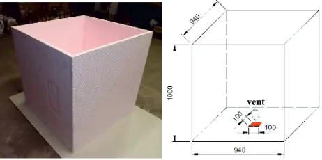
Measurement was performed in a defined space of a cube shape confined with polystyrene panels with an area of 0.5 m2 and thickness of 0.03 m.
Figure 1. Geometry of experimental space. vent C
Owned by the authors, published by EDP Sciences, 2014
Inside volume of a vessel is 0.8836 m3. Figure 1 demonstrates the geometry of experimental space. At the bottom side, there is an opening for balancing of arisen overpressure in a vessel at gas leak and ambient atmosphere.
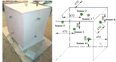
For measurement of gas concentration, methane detectors type CH4-GC20N were installed in vessel walls [7,9]. Figure 2 shows general arrangement of a whole measuring setup. Sensors are marked as green points.
Figure 2. Layout of measuring sensors.
Gas flows through the sample to predefined leakage. Gas leaks out through it to internal space confined with vessel’s walls. All samples were made so that the leakage is always situated in the middle of the bottom in height of 250 mm. Measurements were taken for three different directions of rotation of a pipe with leakages. The first one is horizontal direction (rotation of leakage is under the angle of 0° to the front of the vessel), the second is inclined direction (angle 45°) and the third one is vertical direction (gas leaks out of the pipe upwards under the angle of 90°) [5].
2.1.2 Samples of fittings with damage
Gas pipe or more precisely predefined sample with defined leakage leads through the opening at the lower part of the side wall. Samples of leakage or damage are specified on the basis of analysis of frequency of typical damages of domestic low pressure pipe occurred in practice.
Experiments were carried out on the set of pipes of equal dimensions differing in a characteristic of opening for gas leak. The end of pipe is closed with blind. Typical geometry of the pipe is introduced in figure 3.
Figure 3. Geometry of testing pipe with leakage
Samples are connected to domestic gas pipe with maximum pressure of about 2 kPa. Amount of leak gas depends mainly on parameters of the opening for gas leak and on pressure in the gas pipe. Within the experiments, eight samples of fittings with defined damage were used.
Sample 1 is represented by nozzle of diameter 0.5 mm. The nozzle of a gas cooker is soldered to the opening that is drilled into a copper gas pipe. The nozzle is a part of gas cookers “Mora”. Opening area is 1.963E-07 m2. Figure 4 presents the shape and geometry of the nozzle.
Figure 4. Shape and geometry of the nozzle.
The same shapes of nozzles are used for samples 2 and 3. Opening areas are 3.32E-07 m2 and 7.85E-07 m2 [4]. Sample 4 is formed with cylindrical opening of diameter 1 mm. The shape of this sample is shown in figure 5. Opening area 7.85E-07 m2 is the same as sample 3.
Figure 5. Shape and geometry of sample 4.
Sample 5 represents longitudinal opening of area 6.694E-05 m2 [4]. This opening was created using rotary saw. Due to opening irregularity, calculation of area is simplified considering two rectangles and five triangles see figure 6.
Figure 6. Shape and geometry of sample 5.
Besides openings with exactly defined areas, a leakage was considering where its area is very difficult to define. Practically it concerns for example wrongly sealed connection on pipe. At the end of pipe, such connection was simulated by screwed blind that was tightened just by hand. This sample is illustrated in figure 7.
Figure 7. Shape and geometry of sample 6.
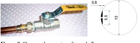
Practically, gas leak can also occur in wrongly closed spherical valve. Imperfect closure can happen for example due to solid contaminant. It was simulated using a needle of diameter 0.6 mm which was inserted between valve body and spherical enclosure. The area of gas leak was calculated with simplification again. Black colour in following figure represents the area of leakage in the shape of segment without area of needle. Final area is 1.791E-05 m2. Valve type and imperfect closure area at sample 7 are shown in figure 8.
Vent
Sensor 4
Sensor 6
Sensor 1 Sensor 5
Sensor 2
Figure 8. Shape and geometry of sample 7.
In the case of sample 8, lateral damage of a gas tube is considered. The gas tube consists of several layers as it is seen in figure 9. Gas goes through the rubber tube with copper fibre leading along this tube. The upper layer is formed of metal braid coated with plastic. For determination of leakage area at the rubber tube, a needle (thickness 0.6 mm) was inserted into the opening. The opening area was calculated from surface of a part of an ellipsoid. A width of a cut is consistent with the needle thickness. Final area is 4.08E-06 m2.
Figure 9. Shape and geometry of sample 8.
2.2 Measurement procedures
At the gas leak to the vessel, times from the start of the gas leak to the sensors reactions were monitored. From measured times, the time period was determined when 10 % and 20 % concentrations of lower explosive limit were reached at measured points. Measurement results show approximate picture of the natural gas leak after leakage from the low pressure gas pipe. Several issues were measured: amount of a leak gas, barometric pressure, gas pressure in a gas distribution system and ambient temerature, but also times from the start of the gas leak to the moments when detectors detected given concentration (0.5 % and 1 % volume concentration). Each measurement was repeated three or four times [10]. Table 1 presents the averages of measured times.
Table 1. Reaction times of detectors.
S a m p l e Flow (45°) Reaction time (s)
Sensor 1 Sensor 2 Sensor 3 Sensor 4 Sensor 5 Sensor 6 0,5 % 1 % 0,5 % 1 % 0,5 % 1 % 0,5 % 1 % 0,5 % 1 % 0,5 % 1 % 1 264 514 222 435 389 626 723 1029 250 342 178 259 2 203 402 217 374 209 378 524 728 157 205 139 201 3 7 72 56 110 76 141 212 306 56 127 56 105 4 9 74 60 138 76 148 237 341 59 132 47 130 5 2 3 5 7 13 15 53 62 6 7 6 8 8 10 13 21 33 27 45 100 120 25 36 44 70
2.3 Measurement results
At this measurement, the same orientation of rotation of the leakage openings was used. The opening were turned to the front side of the vessel with the sensor No. 1. Imaginary straight line, perpendicular to the opening area, formed an angle of 45°. Six samples were measured. figure 10 illustrates the graph with reaction times of the detectors for 0.5 % volume concentration of a natural gas.
Considering these measured times, approximate estimation of a direction of a natural gas expansion after leakage can be done. To make the graph more clear, points (reaction times) are connected with dashed lines.
Figure 10. Gas expansion depending on the leakage type.
Expansion of a gas from openings with larger gas leak was comparable. First, gas expanded to the front side to the sensor No. 1. Then gas expanded almost steady along upper parts of the side walls and along the ceiling. This can be estimated from nearly uniform reactions of all three sensors (No. 2, 5 and 6). Then reaction of the remaining sensor followed. Finally, gas was gathered at the ceiling of the vessel and it was pressed down to the bottom of the vessel (reaction of the sensor No. 4).
Some diversity occurs at smaller openings (nozzles openings of diameters 0.65 and 0.5 mm). Primary gas flow was expected towards the front side but it did not happen. For nozzles of diameter of 0.65 mm, first a gas was flowing to the side walls of the vessel. Not before c. 40 s, the sensors located at the front and back sides of the vessel started to react. Just as the fifth sensor in the sequence, the sensor No. 2 reacted. In the case of the nozzle of diameter 0.5 mm, a gas expanded first up to the ceiling and to the side walls. After longer time, 0.5 % concentration was formed in the upper part of the front wall.
Directions of gas expansion are important due to determination of local explosive concentration of a natural gas which can be formed at accumulation of sufficient amount of a gas in a certain place of a space where leak from the low pressure gas pipe occurs [8]. This paper deals only with rough estimate because only inexact measuring equipment and small amount of detectors were used during testing.
Figure 11 provides a percentage time difference of reactions of single sensors at concentration change from 0,5 % to 1 % of methane.
Figure 11. Percentage comparison of concentration changes between detectors.
Rate of concentration change differs in each sample. In the graph, only one sample is compared each time. At all measurements, the slowest increase of concentration nozzle ø 0.65 mm nozzle ø 1 mm nozzle ø 0.5 mm
longitudinal vent cylindrical vent
tube cut
Sensors
sensor 1 sensor 2 sensor 3 sensor 4 sensor 5 sensor 6
P
ercen
tage (
%
)
nozzle ø 0.65 mm nozzle ø 1 mm
nozzle ø 0.5 mm
occurred at the sample No. 4. Therefore, these values were taken as reference values. Percentage ratios dependent on time of concentration change of the sensor No. 4 (100 %) were attached to other measured times. For the sample No. 1, very fast change at detectors No. 5 and 6 happened (25 to 30 %). Concentration was changed much more slowly at sensors No. 1, 2 and 3 (70 to 80 %). Situation was similar to the sample No. 2. When a natural gas leaked from the cut at the tube, concentration change was the fastest at the sensor No. 1 (15 %). For other sensors, rate of concentration change was quite different and comparable to other samples (3 and 4).
3
Theoretical part – Numerical model
Used mathematical models are given by continuity equation, equations of motion, equations for transfer of turbulent quantities extended for transfer of mass fraction of admixtures, eventually molar concentrations. Transfer of admixtures (of mass friction) is solved using balance equation which in changing time counts with time-centred mean quantities it means mass frictions of present gases and components of flow rate. Diffusion flow of n-th component of the mixture, velocity of admixtures production owing to chemical reaction and velocity of increment production from distributed mixture are considered. Distribution of admixtures differs according to diffusion flow. Generally, diffusion flow is divided to laminar or turbulent flow [1]. In the first step, physical characteristics of single gases from the mixture were determined. In the case of problem with isothermic flow of homogeneous mixture (mixing of substances with constant temperature), their physical properties could be expressed using constant values. Density, viscosity, specific heat capacity, thermal conductivity and standard merging enthalpy and entropy are the properties of gases which are constant at isothermic flow.
Time-dependent problems are very demanding on computational time. Balance equation has to be discretized in time and space. Space discretization for time-dependent equations corresponds to a stationary task. Time discretization includes the integration of each member of differential equation with defined time step. Time step size can be estimated following the character of solved task and number of external iterations in each time step. Calculations usually start with a small time step which is increasing during calculation. Calculation time is affected also by further quantum of factors, for example quality of computational network, number of calculated equations in one time step, setting of calculation accuracy and many others [2].
3.1 Geometry of the model
Geometry of numerical model was developed in Design Modeler software. In this case heat transfer through the wall was not concerned so the thickness of the wall could be ignored and just inside volumes of all parts could be modelled. In the end, this step decreased final number of segments in computational network and accelerated the computational time. Geometry consists of a gas pipe with
leakage of a sample and of volume of a vessel in the cube shape to which defined gas is leaking. For creating of model of measuring setup, the sample No. 4 was chosen (opening with diameter of 1 mm). Due to better meshing of computational section, the inner space was divided into five smaller volumes as it is seen in figure 12.
Figure 12. Model of experimental setup.
3.2 Meshing of the model
Several options of meshing were tried out during creating of sample mesh. Unfortunately, the least exact way was chosen as the most suitable. This meshing uses tetrahedrons which enable to mesh very small leakage (cylinder with diameter and height of 1 mm) and at the same time it keep the optimal ratio between small size of leakage, large ambient computational space and total number of elements in generated computational mesh. In the case of meshing of inner and outer volume of the sample (the pipe), the mesh consists of 40 807 elements.
Figure 13. Computational mesh of experimental setup.
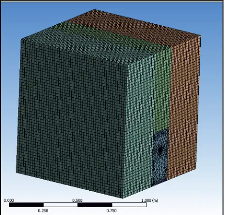
Remaining space without mesh was meshed using extruding function with the help of predefined amount of elements at the edges defining the computational space. Final computational mesh is shown in figure 13. Final mesh consists of 274 426 elements and a parameter for determination of quality of 3D cell (its deformation ratio) is 0.748.
At the places of gas detectors in experimental vessel, in numerical model monitoring points „Surface monitors“ were entered. Therefore, mesh were refined close to all sensors and created leakage as it is illustrated in figure 14.
Figure 14. Refinement of mesh.
3.3 Flow models and boundary conditions
Assessed case represents pass between laminar and turbulent flow when laminar flow (Re = 359) proceeds in the pipe and at the medium leak from the leakage Reynolds number increases to 4640. So turbulent flow occurs. In specific distance of the leakage, a gas expands with low velocity and pressure. Six mathematical models were chosen and compared to the practical measurement.
The first model was chosen as a laminar. This model is advantageous due to faster debugging and testing of calculation with various parameters. High inaccuracy is disadvantage of this model.
The „k-İ RNG“ was chosen as the second model. The RNG method is used very often and it is more accurately compared to other mathematical models mainly in whirling areas where transferred medium is slowing down and lower Reynolds number occurs.
Other used models (k-İ Standard; k-İ Realiable; k-Ȧ Standard and k-Ȧ SST) are common used models for solution of engineering tasks [6].
All boundary conditions were taken from the experiments. Boundary conditions involve mainly setting of fixed obstructers (pipe and vessel walls) and place and intensity of gas entering and leaking from the setup. Walls of the pipe and the vessel were defined with type “wall”. At turbulence models, input and output boundary conditions were defined with the help of turbulence intensity and hydraulic diameter. In the gas pipe (gas entry) the velocity of a gas flow was low therefore the value of turbulence intensity was 1 %. Hydraulic diameter means the inner diameter of the pipe (0.013 m). Flow through the opening at the bottom of the vessel (gas exit) was defined with 0% intensity and hydraulic diameter of 0.1 m.
4 Results
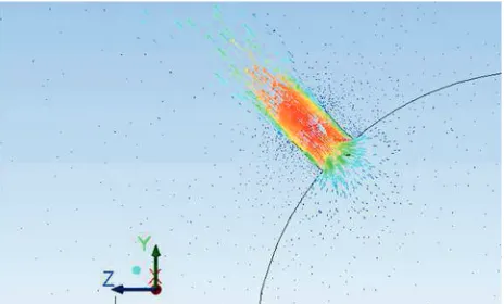
Efflux velocity of a gas from the pipe is one of the important parameters that have to be determined for detection of intensity of gas leak from the opening to the open space. Flow velocity was constant for all efflux area and it was 71.3 m/s. Literature [7] mentions uniform velocity of efflux from the leakage for low pressure gas pipes as 75 m/s. Figures 15 and 16 illustrates the vectors of efflux velocities determined by ANSYS Fluent software. These vectors are moving from c. 40 m/s (right before the entry to and at the edges of the opening) to 79.8 m/s in the middle of the opening. In the right part of the figure, fast decrease of velocity is apparent even for such a small distance from the opening. Vectors behind the opening represent velocities of sucked air.
Figure 15. Efflux velocities (cross-section through the opening in the pipe).
Software also enables to show the arrangement of densities, static, dynamic and total pressure or the size of turbulent quantities in different places of numerical setup. Then it is possible to determine the places with whirling or with suction (self-suction of a gas).
Figure 16. Efflux velocities (complex wiev).
compared to measurements. Figure 17 shows dependence of concentration change on reaction time at sensor No. 1.
Figure 17. Dependence of concentration change on time at the sensor No. 1.
Figure 18 imagines dependence of concentration change on reaction time at the detector No. 2.
Figure 18. Dependence of concentration change on time at the sensor No. 2.
Figure 19 introduce dependance of concentration change on reaction time at the sensor No. 3.
Figure 19. Dependence of concentration change on time at the sensor No. 3.
Figure 20 picture dependence of concentration change on reaction time at the detector No. 4.
Figure 20. Dependence of concentration change on time at the sensor No. 4.
Dependence of concentration change on reaction time at the detector No. 5 is shown in figure 21.
Figure 21. Dependence of concentration change on time at the sensor No. 5.
Figure 22 presents dependence of concentration change on reaction time at the detector No. 6.
Figure 22. Dependence of concentration change on time at the sensor No. 6.
For following evaluation of methane expansion in the inside space of the vessel, model of turbulent flow „k-İ Standard“ was chosen. This model proved the best agreement with the experiments results.
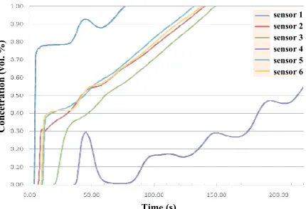
Figure 23 shows the dependence of concentration change on reaction time at all sensors for chosen model of turbulent flow.
laminar_model kȦ_standard_model kȦ_SST_model kİ_standard_model kİ_realiable_model kİ_RNG_model experiment
Time (s)
Con
cet
rat
ion
(
v
ol
. %)
Time (s)
Time (s)
laminar_model kȦ_standard_model kȦ_SST_model kİ_standard_model kİ_realiable_model kİ_RNG_model experiment laminar_model kȦ_standard_model kȦ_SST_model kİ_standard_model kİ_realiable_model kİ_RNG_model experiment_1
Con
cet
rat
ion
(
v
ol
. %)
C
oncetrat
ion (v
ol.
%)
laminar_model kȦ_standard_model kȦ_SST_model kİ_standard_model
kİ_realiable_model
kİ_RNG_model experiment Time (s)
Time (s)
Time (s)
laminar_model kȦ_standard_model kȦ_SST_model kİ_standard_model kİ_realiable_model kİ_RNG_model experiment
laminar_model kȦ_standard_model kȦ_SST_model kİ_standard_model kİ_realiable_model kİ_RNG_model experiment_1 experiment_2
Con
cet
rat
ion
(
v
ol
. %)
Con
cet
rat
ion
(
v
ol
. %)
Con
cet
rat
ion
(
v
ol
Figure 23. Dependence of concentration change on reaction time for all installed sensors.
Considering graphs above, comparably fast expansion of a natural gas along the ceiling and upper parts of side walls (sensors 2, 5 and 6) is visible. At specific moment, velocity of increase of mixture concentration at the ceiling of the vessel starts to slow down which is not fully valid for velocity of gas expansion along the side walls. Before the concentration of 0.5 % is reached, flow alines in all three directions and sensors react approximately equally.
5 Conclusion
Considering graphs in figures 16 to 21, high agreement of results from the experiments and numerical models is apparent. Reactions of sensors No. 1, 2, 3 and 5 accord with modelling results. Large divergence is seen at sensors 4 and 6. Testing of models changed mainly the monitoring point (sensor) No. 4. Before changes, 0.5 % and 1% concentration occurred at „k-Ȧ“ models approximately 140 second sooner than at the experiment. For „k-İ“ models, concentrations occurred c. 80 second sooner than at the experiment. After testing the model, differences between measurement and calculations shortened to 80 s (k-Ȧ models) and 20 s (k-İ models). It means that for areas with very low level of flow it is necessary to define in detail boundary conditions of the models. Even models modification did not lead to requested agreement between measurements and calculations around sensor No. 6. Measurement agreed with models regarding velocity of change from 0.5 % to 1% concentration but it did not agreed with reaction times „experiment_1“. On the basis of numerical model, assumption of wrong functioning of the sensor 6 arose. For repeated measurements, the detector was changed. Measurement results after changing of the sensor are shown in figure 21. (line “experiment_2”). Results agreed so it could be stated that numerical model corresponds to experiment.
Generally, results show that in the beginning concentration is increasing intensely and approximately at 0.3 % to 0.5 % concentration, the methane concentration increases slowly in watched places. Only at the fourth monitored point, rapid increase is followed by rapid repeated decrease of concentration. After several seconds slow increase occurs. At the point No. 4, light
decrease of concentration is visible just before or after 0.5 % concentration is reached. This phenomenon agrees with measurement because at several measurements diode signaling 0.5 % concentration really just blinked and only after a while it lighted permanently.
References
1. Ansys, Inc. ANSYS FLUENT 13.0 - Theory Guide. (2010)
2. M. Bojko, 3D Flow – ANSYS Fluent: textbook (in Czech). 1. issue. Ostrava: Edit centre VŠB – TUO, (2012)
3. C.J.H. Bosch, N.J. Duijm, Methods for the calculation of physical effects CPR 14E. Third edition. Hague : Committee for the Prevention of Disasters, Outflow and Spray release, 2.1-2.179, (2005)
4. J. Fík, Natural gas: tables, diagrams, equations, calculations. Praha : Agentura ýSTZ, s.r.o., 355, (2006)
5. V. Koza, L. ýapla, Determination of leak gas amount from damaged gas pipes. Gas: professional periodical for gas manufacture. Vol. XC, 2, 38-42, (2010)
6. M. Kozubková, Modelling of liquids flow, FLUENT, CFX. 1. issue. Ostrava: Edit centre VŠB – TUO, (2008)
7. Manual KW 9007 of company I.T. WORKS, 92, (2011)
8. TDG 903 01 – Calculation of leak gas amount from damaged gas pipes and gas connections, ýPS, (2006) 9. Technical conditions and service manual for
detectors GC20N and GC20K, 8, (2002)
10. A. Tulach, Determination of the Amount of Natural Gas Leaked from the Internal Gas Supply Piping. Diploma thesis. Ostrava: VŠB-TU Ostrava, 67, (2013)
Time (s)
sensor 1 sensor 2 sensor 3 sensor 4 sensor 5 sensor 6
Con
cet
rat
ion
(
v
ol