Heterogeneity issues in the meta-analysis of cluster randomization trials.

(1)

Scholarship@Western

Electronic Thesis and Dissertation Repository

5-29-2012 12:00 AM

Heterogeneity issues in the meta-analysis of cluster

randomization trials.

Shun Fu Chen

The University of Western Ontario

Supervisor Drs Allan Donner

The University of Western Ontario Joint Supervisor Neil Klar

The University of Western Ontario

Graduate Program in Epidemiology and Biostatistics

A thesis submitted in partial fulfillment of the requirements for the degree in Doctor of Philosophy

Follow this and additional works at: https://ir.lib.uwo.ca/etd

Part of the Biostatistics Commons, and the Clinical Trials Commons

Recommended Citation Recommended Citation

Chen, Shun Fu, "Heterogeneity issues in the meta-analysis of cluster randomization trials." (2012). Electronic Thesis and Dissertation Repository. 572.

https://ir.lib.uwo.ca/etd/572

This Dissertation/Thesis is brought to you for free and open access by Scholarship@Western. It has been accepted for inclusion in Electronic Thesis and Dissertation Repository by an authorized administrator of

(2)

Thesis format: Monograph

by

Shun Fu Chen

Graduate Program in Epidemiology & Biostatistics

A thesis submitted in partial fulfillment of the requirements for the degree of

Doctor of Philosophy

The School of Graduate and Postdoctoral Studies The University of Western Ontario

London, Ontario, Canada

c

(3)

THE UNIVERSITY OF WESTERN ONTARIO

THE SCHOOL OF GRADUATE AND POSTDOCTORAL STUDIES

Joint-Supervisor

Dr. Allan Donner

Joint-Supervisor

Dr. Neil Klar

Examiners

Dr. Shelley Bull

Dr. Yun-Hee Choi

Dr. John Koval

Dr. Serge Provost

The thesis by

Shun Fu Chen

entitled

HETEROGENEITY ISSUES IN THE META-ANALYSIS OF CLUSTER RANDOMIZATION TRIALS

is accepted in partial fulfillment of the requirements for the degree of

Doctor of Philosophy

Date

Chair of the Examination Board

(4)

An increasing number of systematic reviews summarize results from cluster randomization

trials. Applying existing meta-analysis methods to such trials is problematic because

responses of subjects within clusters are likely correlated. The aim of this thesis is to

eval-uate heterogeneity in the context of fixed effects models providing guidance for conducting

a meta-analysis of such trials. The approaches include the adjusted Q statistic, adjusted

heterogeneity variance (τ2

c) estimators and their corresponding confidence intervals and

adjusted measures of heterogeneity (H2

a, R2a, Ia2) and their corresponding confidence

intervals. Attention is limited to meta-analyses of completely randomized trials having

a binary outcome. An analytic expression for power of Q test is derived, which may be

useful in planning a meta-analysis. The Type I error and power for the Q statistic, bias

and mean square errors for the estimators and the coverage, tail errors and interval width

for the confidence interval methods are investigated using Monte Carlo simulation.

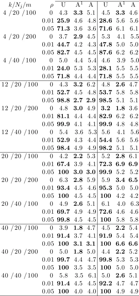
Simulation results show that the adjusted Q statistic has a Type I error close to the

nominal level of 0.05 as compared to the unadjusted Q statistic which has a highly inflated

Type I error. Power estimated using the algebraic formula had similar results to empirical

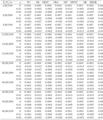
power. For τ_c2 estimators, the iterative REML estimator consistently had little bias.

However, the noniterative MVVC and DLVC estimators with relatively low bias may also

be recommended for small and large heterogeneity, respectively. The Q profile confidence

interval approach for τ2

c had generally nominal coverage for large heterogeneity. The

measures of heterogeneity had generally low bias for large number of trials. For confidence

interval approaches, the MOVER consistently maintained nominal coverage for ‘low’ to

‘moderate’ heterogeneity. For the absence of heterogeneity, the approach based on the Q

statistic is preferred. Data from four cluster randomization trials are used to illustrate

methods of analysis.

Keywords: cluster randomization; meta-analysis; heterogeneity; binary outcome; Q statistic; power; confidence intervals

(5)

First, I would like to express my deepest appreciation to my supervisors, Drs Allan Donner

and Neil Klar, for offering the opportunity to pursue my PH.D studies in Biostatistics

at the Department of Biostatistics and Epidemiology of Univerisity of Western Ontario.

I would also like to thank them for their persistent patience, warm encouragement and

effective guidance while working on the thesis. This thesis would not have been completed

without their continuous help.

I would thank the authors of the four papers (Moher et al., 2001; Woodcock et al., 1999;

Montgomery et al., 2000; Jolly et al., 1999) for use of their data and Dr. Martin Gulliford

for facilitating their use.

With all my affection, I thank my parents, my husband and my son, for their love and

support.

Finally, I thank God to provide all those people in my life who have helped me and prayed

for me to complete this thesis which seems to be impossible years ago.

(6)

CERTIFICATE OF EXAMINATION ii

ABSTRACT iii

ACKNOWLEDGEMENTS iv

CONTENTS v

LIST OF TABLES viii

LIST OF FIGURES xii

1 Introduction 1

1.1 Cluster randomization trials . . . 1

1.2 Meta-analysis of individually randomized trials . . . 2

1.2.1 Fixed versus random effects modeling of heterogeneity . . . 3

1.2.2 Tests of heterogeneity: Q statistic . . . 3

1.2.3 Heterogeneity variance estimatorsτ2 . . . 4

1.2.4 Measures of heterogeneity . . . 7

1.3 Meta-analysis of cluster randomization trials . . . 10

1.4 Scope of thesis . . . 12

1.5 Thesis objectives . . . 14

1.6 Organization of the thesis . . . 15

2 Approximate power of the adjusted Q statistic 16 2.1 Introduction . . . 16

2.2 Notation . . . 17

2.3 Fixed effects model . . . 19

2.3.1 Adjusted Q statistic . . . 19

2.3.2 Approximate power . . . 22

2.4 Summary . . . 27

(7)

3.1 Introduction . . . 29

3.2 Random effects model . . . 30

3.3 Adjusted heterogeneity variance estimators τ2 c . . . 31

3.3.1 Variance component estimator (VC) . . . 31

3.3.2 DerSimonian and Laird estimator (DL) . . . 32

3.3.3 Model error variance estimator (MV) . . . 34

3.3.4 Maximum likelihood estimator (ML) . . . 35

3.3.5 Restricted maximum likelihood estimator (REML) . . . 36

3.4 Confidence intervals for τ2 c . . . 37

3.4.1 Q profile confidence intervals . . . 37

3.4.2 Biggerstaff-Tweedie confidence intervals . . . 37

3.4.3 Profile likelihood confidence intervals . . . 39

3.4.4 Wald-type confidence intervals . . . 39

3.4.5 Sidik-Jonkman confidence intervals . . . 40

3.4.6 Nonparametric bootstraps confidence intervals . . . 41

3.5 Summary . . . 41

4 Measures of heterogeneity 44 4.1 Introduction . . . 44

4.2 Measures of Heterogeneity . . . 45

4.2.1 Quantifying Heterogeneity . . . 45

4.2.2 Adjusted H statistic . . . 47

4.2.3 Adjusted R statistic . . . 48

4.2.4 Adjusted I2 _{statistic . . . .} ₅₀

4.3 Confidence intervals . . . 51

4.3.1 Intervals based on MOVER . . . 51

4.3.2 Intervals based on the distribution of Qa . . . 53

4.3.3 Intervals based on the statistical significance of Qa . . . 53

4.3.4 Intervals based on the estimation of τ2 c . . . 54

4.3.5 Bootstraps confidence intervals . . . 54

4.4 Summary . . . 55

5 Simulation study design 56 5.1 Introduction . . . 56

5.2 Objectives . . . 57

5.3 Selection of parameters . . . 57

5.4 Generation of data . . . 61

5.5 Evaluation criteria . . . 62

(8)

6.2 Adjusted Q statistic . . . 66

6.2.1 Type I error . . . 66

6.2.2 Power . . . 67

6.3 Heterogeneity variance estimators . . . 69

6.3.1 Convergence issues . . . 70

6.3.2 Comparing bias and mean square error . . . 70

6.3.3 Confidence interval approaches . . . 72

6.4 Measures of heterogeneity . . . 74

6.4.1 Bias and mean square error . . . 74

6.4.2 Confidence interval approaches . . . 75

6.5 Discussion . . . 77

7 Meta-analysis of practice-based secondary prevention programs for pa-tients with heart disease risk factors 126 7.1 Introduction . . . 126

7.2 Aspects of Study Data . . . 127

7.3 Method of analysis . . . 129

7.4 Results . . . 131

7.5 Summary . . . 132

8 Conclusions 136 8.1 Introduction . . . 136

8.2 Summary . . . 137

8.2.1 Key findings . . . 137

8.2.2 Recommendations . . . 139

8.2.3 Practical issues . . . 140

8.3 Limitations and future research . . . 141

A Derivation of Q statistic 145

B Intracluster correlation coefficient (ANOVA estimator) 148

C Variance component approach 150

D ML approach 151

E REML approach 154

BIBLIOGRAPHY 156

VITA 162

(9)

List of Tables

1.1 Summary of the heterogeneity variance estimators . . . 6

2.1 Data layout for a meta-analysis of k cluster randomized trials. . . 18

2.2 Notation used in Table 2.1 . . . 18

2.3 Responses for the jth trial . . . 20

3.1 Summary of the adjusted heterogeneity variance estimators with the meth-ods of constructing confidence intervals . . . 43

4.1 Degree of Heterogeneity . . . 55

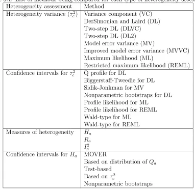
5.1 List of methods being compared for each type of heterogeneity assessment. 58 5.2 Simulation parameters for cluster randomization simulation study . . . . 60

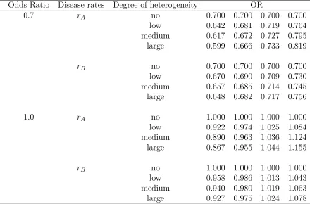
5.3 List of odds ratio values to generate clustered binary datasets. . . 61

6.1 Type I error (%) of Q statistic for odds ratio ψ = 0.7 based on 1000 simulations. . . 80

6.2 Type I error (%) of Q statistic for odds ratio ψ = 1.0 based on 1000 simulations. . . 81

6.3 Power (%) of adjusted Q statistic for odds ratioψ = 0.7 with truncated ρ based on 1000 simulations. . . 82

6.4 Power (%) of adjusted Q statistic for odds ratioψ = 1.0 with truncated ρ based on 1000 simulations. . . 83

6.5 Power (%) of adjusted Q statistic for odds ratioψ = 0.7 omitting truncation based on 1000 simulations. . . 84

6.6 Power (%) of adjusted Q statistic for odds ratioψ = 0.7 omitting truncation based on 1000 simulations. . . 85

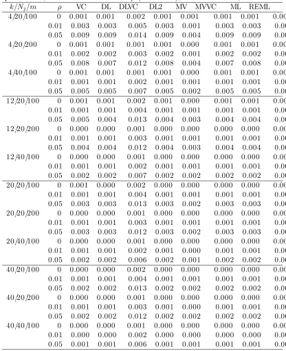
6.7 Bias forτ2 c with ‘no’ heterogeneity and control group disease ratesrAbased on 1000 simulations. . . 86

6.8 Bias for τ2 c with ‘low’ heterogeneity and control group disease rates rA based on 1000 simulations. . . 87

6.9 Bias for τ2 c with ‘moderate’ heterogeneity and control group disease rates rA based on 1000 simulations. . . 88

(10)

6.11 Bias for τ2

c with ‘no’ heterogeneity and control group disease ratesrB based

on 1000 simulations. . . 90

6.12 Bias for τ2

c with ‘low’ heterogeneity and control group disease rates rB

based on 1000 simulations. . . 91

6.13 Bias for τ_c2 with ‘moderate’ heterogeneity and control group disease rates

rB based on 1000 simulations. . . 92

6.14 Bias for τ_c2 with ‘high’ heterogeneity and control group disease rates rB

based on 1000 simulations. . . 93

6.15 Confidence intervals for τ2

c with ‘no’ heterogeneity, control group disease

ratesrA for Q profile(PQ), Biggerstaff-Tweedie(BT), Sidik-Jonkman(SJ)

and nonparametric bootstraps(NB) based on 1000 simulations . . . 94

6.16 Confidence intervals for τ_c2 with ‘no’ heterogeneity, control group disease

rates rA for profile likelihood and Wald-Type based on 1000 simulations . 95

6.17 Confidence intervals for τ_c2 with ‘low’ heterogeneity, control group disease

c with ‘low’ heterogeneity, control group disease

6.19 Confidence intervals for τ_c2 with ‘moderate’ heterogeneity, control group

dis-ease ratesrAfor Q profile(PQ), Biggerstaff-Tweedie(BT), Sidik-Jonkman(SJ)

c with ‘moderate’ heterogeneity, control group

disease ratesrAfor profile likelihood and Wald-Type based on 1000 simulations 99

c with ‘high’ heterogeneity, control group disease

c with ‘no’ heterogeneity, control group disease

ratesrB for Q profile(PQ), Biggerstaff-Tweedie(BT), Sidik-Jonkman(SJ)

6.24 Confidence intervals for τ_c2 with ‘no’ heterogeneity, control group disease

rates rB for profile likelihood, and Wald-Type based on 1000 simulations 103

(11)

ease ratesrBfor Q profile(PQ), Biggerstaff-Tweedie(BT), Sidik-Jonkman(SJ)

c with ‘moderate’ heterogeneity, control group

disease rates rB for profile likelihood, and Wald-Type based on 1000

simulations . . . 107

6.30 Confidence intervals for τ_c2 with ‘high’ heterogeneity, control group disease

6.31 Bias and MSE for the measures of heterogeneity with ‘no’ heterogeneity

and control group disease ratesrA based on 1000 simulations . . . 110

6.32 Bias and MSE for the measures of heterogeneity with ‘low’ heterogeneity

6.33 Bias and MSE for the measures of heterogeneity with ‘moderate’

hetero-geneity and control group disease rates rA based on 1000 simulations . . 112

6.34 Bias and MSE for the measures of heterogeneity with ‘high’ heterogeneity

6.35 Bias and MSE for the measures of heterogeneity with ‘no’ heterogeneity

and control group disease ratesrB based on 1000 simulations . . . 114

6.36 Bias and MSE for the measures of heterogeneity with ‘low’ heterogeneity

6.37 Bias and MSE for the measures of heterogeneity with ‘moderate’

hetero-geneity and control group disease rates rB based on 1000 simulations . . 116

6.38 Bias and MSE for the measures of heterogeneity with ‘high’ heterogeneity

6.39 Confidence interval for Ha with ‘no’ heterogeneity, control group disease

rates rA for MOVER, Q distribution, test-based, based onτc2,

nonparamet-ric bootstrap based on 1000 simulations . . . 118

6.40 Confidence interval for Ha with ‘low’ heterogeneity, control group disease

6.41 Confidence interval for Ha with ‘moderate’ heterogeneity, control group

disease rates rA for MOVER, Q distribution, test-based, based on τc2,

nonparametric bootstrap based on 1000 simulations . . . 120

6.42 Confidence interval for Ha with ‘high’ heterogeneity, control group disease

6.43 Confidence interval for Ha with ‘no’ heterogeneity, control group disease

rates rB for MOVER, Q distribution, test-based, based onτc2,

(12)

ric bootstrap based on 1000 simulations . . . 123

6.45 Confidence interval for Ha with ‘moderate’ heterogeneity, control group

disease rates rB for MOVER, Q distribution, test-based, based on τc2,

nonparametric bootstrap based on 1000 simulations . . . 124

6.46 Confidence interval for Ha with ‘high’ heterogeneity, control group disease

rates rB for MOVER, Q distribution, test-based, based onτc2,

7.1 Description of studies. . . 127

7.2 Baseline characteristics of patients in intervention groups for each trial

included in the meta-analysis. . . 130

7.3 Heterogeneity variance estimators and random effects summary odds ratios .133

7.4 Point estimates and confidence intervals forτ2

c. . . 133

7.5 Confidence intervals for Ha. . . 134

(13)

List of Figures

2.1 Approximate power of Qa plotted against τc2 (first column) and ρ (second

column). . . 28

4.1 Estimated Ha plotted against degree of heterogeneity. . . 49

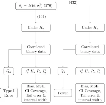
5.1 Flowchart of the simulation study. Number of parameter combination is

noted in parentheses. . . 65

7.1 Forest plot for the meta-analysis of practice-based secondary prevention

programs for patients with coronary heart disease risk factors. . . 131

(14)

Chapter 1 Introduction

1.1 Cluster randomization trials

Randomized controlled trials are often deemed the gold standard to assess the effectiveness

of an intervention in health research (Wade, 1999). A key benefit of randomization is

the potential for elimination of bias due to confounding. The units of randomization in

randomized trials are usually the individual.

Over the past two decades, randomized trials in which the unit of randomization is at the

cluster level have been more frequently adopted in the evaluation of health care

interven-tions, screening and educational programs (Bland, 2004). Such trials are characterized

by random assignment of intact social units (e.g., worksites, clinical practices, schools or

entire communities) instead of individual study subjects (Donner and Klar, 2000).

For example, a study evaluating the effect of vitamin A supplementation on childhood

mortality (Sommer et al., 1986) adopted cluster randomization because it was not

po-litically feasible to randomize individuals. Hence, the units of randomization for this

study were villages instead of individuals within a village. Contamination could have

(15)

individuals from the same village who were assigned to different interventions shared their

vitamin A supplement. Cluster randomization trials are preferred in situations where

the ethical issues, the desire to control costs or the attempt to minimize experimental

contamination are major concerns.

However, the cluster randomization design is statistically less efficient compared to

in-dividual randomization because responses of inin-dividuals in a cluster tend to be more

similar to each other than to responses of individuals in different clusters. The degree of

similarity is measured using the intracluster correlation coefficient denoted by ρ (Donner

and Klar, 2000, p2) which takes a value between 0 and 1. In order to adjust for clustering,

the variance of the estimated intervention effect is multiplied by a variance inflation factor

(or design effect), IF = 1 + ( ¯m+ 1)ρ where ¯m is the average cluster size. Intracluster

correlation coefficients may be quite small particularly for community intervention trials

where they rarely take on values above 0.1 (Murray et al., 2000). However even then

design effects may be quite large since such trials typically recruit hundreds of subjects

per cluster. Subsequently, ignoring clustering effects could result in spurious statistical

significance where the variance estimators will tend to be underestimated.

1.2 Meta-analysis of individually randomized trials

Since the 1980s there have been a growing number of published systematic reviews

sum-marizing results from clinical trials (Whitehead, 2002, page xiii). At the same time, there

has also been increasing methodological research dealing with meta-analytic methods.

A key challenge in combining study results is possible heterogeneity in the estimated

intervention effect. Heterogeneity may reflect systematic differences in study design or

in characteristics of participating subjects or may be a consequence of random variation

(16)

1.2.1 Fixed versus random effects modeling of heterogeneity

Fixed effects and random effects models depend on different assumptions about

hetero-geneity of the intervention effect. The fixed effects model assumes that there is a common

fixed effect (at least for interval estimation) and a random component (sampling error)

that is responsible for differences among trial results. Often, however, there may be some

heterogeneity of intervention effects across trials. A test of heterogeneity is frequently

used to evaluate the assumption of a common fixed effect. On the other hand, the random

effects model assumes that the observed trials are a random sample from a hypothetical

population of trials. To account for the variation among trial results, an additional

random term is added to the model. This added term, recognized as the heterogeneity

variance parameter, is denoted byτ2. Consequently, the random effects model generally

yields more conservative inferences about the intervention effect as compared to the fixed

effects model (Schulze, 2007; Villar et al., 2001).

1.2.2 Tests of heterogeneity: Q statistic

The Q statistic (Cochran, 1954) tests the null hypothesis: Ho :θ1 = θ2 = . . .=θk =θ

versus the alternativeHA: at least one trial had a truly different intervention effect as

com-pared to the other trials, where θj denotes the intervention effect for trial j, j = 1, . . . , k.

Mathematically, the Q statistic is defined as a weighted sum of squares of the deviations

of individual study estimates ˆθj, from the overall estimate ˆθ. The Q statistic when Ho is

true, is approximately a chi-square random variable with k₋1 degrees of freedom. If

the null hypothesisHo is rejected, one concludes that there is at least one study which

truly differs from other studies in terms of the intervention effect. Further analyses are

then usually recommended to identify covariates that stratify studies into homogeneous

(17)

Several other test statistics are available to test for heterogeneity (e.g. likelihood ratio

test, score test). In a simulation study generating continuous outcome data, Viechtbauer

(2007b) showed that the Q statistic as compared to other test statistics kept the tightest

control of the Type I error rate for meta-analyses based on studies having at least

moder-ately large sample size, such that the number of trials is from 5 to 80 and the average

sample size per trial is 20 to 640. He also suggested that if the amount of heterogeneity

was small, sample sizes exceeding 100 observations within each study would be required

to detect it. As for binary outcome data in large sample sizes, the Q statistic based on

the Woolf estimator is conservative in general and least powerful for severely unbalanced

and within-strata unbalanced designs (Paul and Donner, 1989). However, for balanced

and mildly unbalanced designs, the Q statistic, which is easy to calculate, is recommended.

According to Hardy and Thompson (1998), the Q statistic may detect clinically

unim-portant heterogeneity when there are many studies but is unable to detect clinically

significant heterogeneity when there are few studies. Therefore, power calculations for the

Q statistic prior to conducting a meta-analysis may prove helpful in assessing statistical

power (Hedges and Pigott, 2001; Valentine et al., 2010). Power for the Q statistic is a

function of the selected effect measure, the specified Type I error, number of trials and

sample size per trial.

1.2.3 Heterogeneity variance estimators

τ

2

Point estimation

Heterogeneity variance estimators are also useful in assessing heterogeneity in

meta-analysis. Their advantage is that they do not depend on the number, or size of trials

in a meta-analysis like the Q statistic. A disadvantage they share with the Q statistic

(18)

measures (e.g. odds ratio, risk ratio and hazard ratio) (R¨ucker et al., 2008). Seven

methods of estimating the parameter τ2 _{were compared in terms of bias and mean square}

error under a random effects model for a binary outcome in a simulation study Sidik and

Jonkman (2007). Four of these estimators are simple to compute while the remaining

three approaches require relatively extensive computation.

Hedges (1983) originally developed a method of moments estimator obtained by setting

the usual sample variance equal to its expected value and solving for τ2, known as the

variance component type estimator. Another method of moments estimator proposed by

DerSimonian and Laird (1986) using the expectation of the Q statistic (Cochran, 1954) is

commonly used in random effects meta-analysis (Brockwell and Gordon, 2001; Thompson

and Sharp, 1999). Furthermore, given that the DerSimonian and Laird estimator often

underestimates the true value (e.g., Bohning et al., 2002; DerSimonian and Kacker, 2007;

DerSimonian and Laird, 1986; Sidik and Jonkman, 2007), DerSimonian and Kacker (2007)

proposed a two-step method to avoid using iterative methods (e.g. likelihood approaches).

Besides the method of moments estimators, Sidik and Jonkman (2005) proposed an

estimator based on the unbiased estimation of the error variance in a linear model, called

a model error variance type estimator. The model error variance type of estimator requires

an initial estimate of τ2_{. The simplest is to use the empirical variance estimate as an}

initial estimator for τ2. Later, Sidik and Jonkman (2007) suggested an improved version

of this approach by using the variance component type estimate as an initial estimate of

τ2. The common iterative approaches to estimatingτ2 are maximum likelihood estimation

and restricted maximum likelihood estimation (Hardy and Thompson, 1996; Harville,

1977; Raudenbush and Bryk, 1985). Another iterative approach is obtaining by using the

empirical Bayes estimator (Morris, 1983).

F

(19)

com-Table 1.1: Summary of the heterogeneity variance estimators

Method Description Non-Iterative

Variance Component (VC) Method of moments

DerSimonian and Laird (DL) Method of moments

Two-step DL (DLVC) Empirical variance as an initial estimator

Two-step DL (DL2) Variance component as an initial estimator

Model Error Variance (MV) Empirical variance as an initial estimator

Improved (MVVC) Variance component as an initial estimator

Iterative

Maximum Likelihood (ML) Likelihood

Restricted (REML) Likelihood

Bayes Bayesian

ponent type estimator and the empirical Bayes estimator provide the most accurate

estimation when the heterogeneity is moderate to large (i.e. τ2 _≥ 0.5). The variance

component estimator and the model error variance both tend to overestimate the true

heterogeneity variance except for meta-analyses with large number of trials and unless

the heterogeneity variance is large, respectively. However, the likelihood estimators and

DerSimonian and Laird’s estimator tend in general to underestimate the true heterogeneity

variance. Schlattmann (2009, Chapter 7) found similar results. Table 1.1 provides a

summary of the heterogeneity variance estimators mentioned above.

Interval estimation

It is often useful to report a confidence interval in addition to a point estimator of

τ2_{. Viechtbauer (2007}_a_{) proposed a new method called the Q profile to construct such}

intervals and evaluated its performance in terms of nominal coverage as compared with

other existing approaches, including Biggerstaff-Tweedie (Biggerstaff and Tweedie, 1997),

profile likelihood, Wald-type, Sidik-Jonkman (Sidik and Jonkman, 2005), parametric

bootstrap and non-parametric bootstrap using Monte-Carlo simulation.

(20)

free-dom under the null hypothesis. Alternatively, the 95 percent confidence interval obtained

from the Q profile method is constructed based on the 2.5th and 97.5th percentile of this

distribution. Based on a similar idea, the Biggerstaff-Tweedie confidence interval can be

obtained by approximating the distribution of Q with a gamma distribution (Biggerstaff

and Tweedie, 1997). For the profile likelihood method, the confidence intervals can

be obtained by profiling the likelihood ratio statistic with the maximum likelihood or

restricted maximum likelihood estimates. Then, the inverse of the Fisher information

matrix is used to calculate the asymptotic sampling variances of the maximum likelihood

and restricted maximum likelihood estimates of the heterogeneity estimator in order to

construct Wald-type confidence intervals. The confidence interval for the model error

variance is based on the assumption that its estimator approximately follows a chi-square

distribution withk₋1 degrees of freedom (Sidik and Jonkman, 2005). Last is the

boot-strap confidence interval constructed by taking the 2.5th and 97.5th empirical percentiles

of the heterogeneity estimate based on the bootstrap sample after repeating the same

process up to 1000 times.

According to simulation results (Viechtbauer, 2007a), the profile likelihood method with

the Q statistic yields the most accurate coverage, closely followed by Biggerstaff and

Tweedie’s method. The performance of other methods was poor in general with a coverage

probability either too low or too high.

1.2.4 Measures of heterogeneity

Higgins and Thompson (2002) proposed three statistics which measure the impact of

heterogeneity on a meta-analysis: H, R, and I2_{. The advantage of these measures as}

compared to the heterogeneity variance is that they allow heterogeneity of the intervention

effect to be compared across meta-analyses including different numbers of studies and

(21)

The H statistic is given by the square root of the Q statistic divided by its degrees of

freedom. Since the expectation of Q is equal to k₋1 under Ho,H = 1 indicates that the

intervention effects are homogeneous across trials. Values of H exceeding 1.5 may suggest

heterogeneity complicating interpretation of the summary estimates of the intervention

effect. The R statistic is the ratio of the standard error of a random effects meta-analytic

summary estimate to the standard error of a fixed effects meta-analytic summary estimate.

It describes the inflation in the confidence interval for a summary intervention effect

estimate under a random effects model compared with a fixed effects model. When the

value is 1, it indicates that the two models yield identical inferences and the fixed effects

model is sufficient. The I2 _{statistic is interpreted as the proportion of total variation}

in the estimate of an intervention effect that is due to heterogeneity between studies.

When the I2 _{statistic is 0 percent, the variation is considered only due to sampling error}

and not due to heterogeneity. Similarly, an I2 statistic of 20 percent indicates that 20

percent of variability in the trials may be attributed to between-study variation. Several

investigators (e.g. Higgins and Green, 2008; Higgins and Thompson, 2002; Higgins et al.,

2002a) recommend including the H or I2 _{statistics when reporting meta-analyses.}

Several simulation studies (Huedo-Medina et al., 2006; Mittlb¨ock and Heinzl, 2006)

exam-ined the properties of H andI2 _{as a function of the ratio of between and within study}

variances. They concluded that I2 but not H may depend on the number of trials when

that number is small (i.e. k _≤10). In addition, the values of I2 _{may be affected by the}

ratio of between and within study variances rather than the between study variance alone.

Possible approaches for constructing confidence intervals for each measure were also

summarized in the appendix of the Higgins and Thompson’s article (2002): i) based on

the distribution of Q, ii) based on the statistical significance of Q (test-based method),

(22)

bootstrap procedure. In addition, the confidence interval approach known as the method

of variance estimates recovery (MOVER) originally proposed by Zou (2008) may be used

to construct a confidence interval for H by treating it as a ratio of within study and

between study variances (Donner and Zou, 2010).

According to the simulation results presented in Table A1 for the H statistic (Higgins

and Thompson, 2002), it appears that a confidence interval constructed based on the

distribution of Q has coverage close to 100 per cent even with large number of trials k (i.e.

k = 30) except for large heterogeneity. The maximum likelihood, restricted likelihood

and bootstrap confidence intervals have inadequate coverage above nominal for small

heterogeneity and below nominal for large heterogeneity. The coverage of the test-based

confidence interval appears to be conservative in most of the situations except when

significant heterogeneity is present or the number of studies is large. The Pearson type

III confidence interval constructed for the heterogeneity estimator provides good coverage

in all situations, but is complicated to calculate. Finally, the accuracy of MOVER will

depend heavily on the performance of confidence intervals for numerator and denominator

of the given ratio (Schuster and Metzger, 2010, Chapter 11).

In summary, despite the different assumptions and methods regarding the assessment

of heterogeneity among studies, the fixed and random effects approaches in principle

both use weighted averages with only a change in the weights to calculate the overall

mean effect size. When the two modeling approaches yield similar results, the conclusions

based on these results gain credibility. When the intervention effects are considered

homogeneous, the results from both models are identical with the heterogeneity variance

(23)

1.3 Meta-analysis of cluster randomization trials

In response to the frequent use of cluster randomization designs in the health research

field, the need to conduct meta-analyses for such trials becomes increasingly evident and

necessary. The challenge in planning and conducting such a meta-analysis involves the

need for accounting for clustering effects. Not recognizing that the unit of randomization

for cluster randomization trials is at the cluster level with outcome measures collected

and analyzed at the individual level will generally lead to underestimating the variance

due to lack of independence between individuals.

Heterogeneity is recognized as another important analytic issue in performing a

meta-analysis by investigators who have performed separate meta-analyses on trials that involve

very different randomization units. For example, a study was conducted by Fawzi et al.

(1993) to investigate the effect of vitamin A supplementation on child mortality. The

participants of this study were taken from studies of hospitalized children with measles,

as well as other studies involving healthy children participating in community-based

trials. Individual children were assigned to intervention in the four hospital-based trials,

while allocation was by village, district or household in the eight community-based trials.

Therefore, the meta-analysis was performed separately for the hospital-based trials and

the community studies. When the results agree, an important advantage is the confidence

gained that the intervention tested is effective (or ineffective) in more than one setting.

Otherwise, the investigator can further study the impact of different choices of

random-ization unit as part of a sensitivity analysis.

One approach to testing heterogeneity in the meta-analysis of cluster randomized trials is

to use the Q statistic adjusted for clustering discussed in Donner et al. (2001). In principle,

the idea is similar to the Q statistic used to test for heterogeneity in meta-analysis of

individually randomized trials, except its weights are modified to account for clustering to

(24)

described independently by Song (2004), suggesting that the adjusted tests maintained

the nominal significance level in a stimulation study.

Methodological researches on meta-analytic methods involving cluster randomized trials

have mainly focused on fixed effects models. By assuming there is no variation between

studies, there are several statistical approaches that can be applied to a meta-analysis

of cluster randomization trials with a binary endpoint. Statistical methods include the

adjusted Mantel-Haenszel procedures, the ratio estimator approach, the general inverse

variance approach, Woolf procedures and generalized estimating equations (GEE) using

robust variance estimation (Donner et al., 2001).

The adjusted Mantel-Haenszel test statistic (Donner and Klar, 2000) is slightly modified

from the standard Mantel-Haenszel test statistic to account for clustering effects. The null

hypothesis is that the overall odds ratio of all 2x2 tables is equal to one and the test

statis-tic follows approximately a chi-squared distribution with one degree of freedom. The ratio

estimator approach is based on an adjustment of the Mantel-Haenszel chi-square statistic

in which the event rate is regarded as a ratio rather than as a proportion. It was developed

by Rao and Scott (1992) and involves dividing the observed sample frequencies (counts) in

a given study by the estimated design effect. The general inverse variance approach (GIV)

is obtained by combining study estimates in a meta-analysis using a weighted average

of estimated effect measures that are calculated separately for each trial. This approach

is recommended in the guidance provided by the Cochrane Collaboration. The Woolf

procedure, which is best applied with a small number of clusters each of fairly large size,

transforms the intervention odds ratio of each trial to the logarithmic scale in order to

obtain a distribution which is more likely to be normally distributed. Then, the average of

the transformed odds ratios is computed using a weighting scheme originally described by

(25)

Furthermore, a simulation study (Darlington and Donner, 2007) was performed to compare

the unadjusted Mantel-Haenszel method, the adjusted Mantel-Haenszel methods, the

ratio procedure, the general inverse variance, and the Woolf procedure. This simulation

study had two important results. First, the simulation results clearly showed that it is

inappropriate to use the unadjusted Mantel-Haenszel method due to elevated Type I error

rate. Second, the adjusted Mantel-Haenszel method had the greatest power and slightly

outperformed the general inverse variance method since it uses information on the cluster

sizes and intracluster coefficient ρ for each trial, while the general inverse method is a

generic procedure.

1.4 Scope of thesis

Most meta-analytic methods focus on combining study results of individually randomized

trials where observations are independent. Meta-analytic methods for cluster

randomiza-tion trials are largely extensions of meta-analytic methods for individually randomized

trials. However, applying existing meta-analytic methods to handle heterogeneity of

cluster randomized trials is problematic with correlated observations. The rationale for

limiting attention to heterogeneity among studies is that this is a substantial issue for

meta-analysis, since when present it complicates discussion of an overall intervention effect.

This research focuses mainly on binary outcomes because such outcomes have been most

frequently used in cluster randomization trials (Laopaiboon, 2003). There are three

fre-quently used designs in cluster randomization trials: completely randomized, matched-pair

and stratified. The completely randomized design is best suited to trials that have a fairly

large numbers of clusters, whereas matching or stratification is more effective in small

studies (Donner and Klar, 2000). The challenge of extending all methods to stratified and

(26)

simplicity, the discussion will thus be focused on designs where there is a single binary,

cluster-level covariate, i.e., trials where there is one experimental group and one control

group.

In summary, my thesis will focus on exploring and evaluating heterogeneity in the context

of fixed effects models with the aim of providing general guidance in conducting a

meta-analysis of cluster randomization trials. Attention will also be limited to meta-analyses

of community intervention trials which typically enroll a small number of large clusters.

This focus reflects the relatively greater methodological challenge of statistical inferences

when estimates of variance inflation are less precisely estimated. Intervention effects for

binary outcomes will be measured using odds ratio estimators comparing an experimental

(27)

1.5 Thesis objectives

The primary objectives of this research are:

1. Analytics

(a) To extend the Q statistic, as commonly applied to test for heterogeneity in

meta-analyses of individually randomized trials, to the meta-analysis of cluster

randomization trials by specifying a weight accounting for clustering.

(b) To obtain an analytic expression for the power curve of the adjusted Q statistic.

(c) To derive heterogeneity variance estimators and their confidence intervals

accounting for clustering.

(d) To derive measures of heterogeneity and their confidence intervals accounting

for clustering.

2. Simulation

(a) To evaluate the performance of the adjusted Q statistic in terms of Type I error

and statistical power and to compare its power with the proposed formula.

(b) To assess the bias and mean square error for the adjusted heterogeneity variance

estimators and to evaluate the coverage, tail errors and interval width of the

proposed confidence interval methods.

(c) To assess the bias and mean square error for the adjusted measures of

het-erogeneity and to evaluate the coverage, tail errors and interval width of the

proposed confidence interval methods.

3. Example

(a) To illustrate the application of results, both in fixed and random effects models,

(28)

1.6 Organization of the thesis

This thesis includes eight chapters. Chapter 2 extends the Q statistic, as commonly

applied to test for heterogeneity in meta-analyses of individually randomized trials, to the

meta-analysis of cluster randomization trials. An analytic expression for the power of the

Q statistic is derived. The effect on the power of cluster size, number of clusters, degree of

heterogeneity, and magnitude of intracluster correlation is explored. Chapter 3 presents

analytic expressions for the heterogeneity variance estimators adjusted for clustering and

describes approaches for constructing confidence intervals. Chapter 4 presents analytic

expressions for the measures of heterogeneity adjusted for clustering and approaches for

constructing confidence intervals.

Chapter 5 describes the design of a simulation study used to assess the procedures and

to validate analytical findings. Performance is evaluated in terms of Type I error and

statistical power for the Q statistic, bias and mean square error for both heterogeneity

variance estimators and measures of heterogeneity, and coverage for the confidence

inter-vals approaches. Results of the simulation study are described in Chapter 6. Chapter 7

presents a meta-analysis of 4 cluster randomization trials to illustrate the application of the

proposed methods. Finally, Chapter 8 summarizes the main results, the recommendations

(29)

Chapter 2 Approximate power of the adjusted

Q statistic

2.1 Introduction

The Q statistic was introduced in Chapter 1 for meta-analysis of individually randomized

trials. An extension of this statistic was also described for cluster randomization trials.

Applying the Q statistic to a meta-analysis of cluster randomized trials without adjusting

for clustering is problematic because the unadjusted Q statistic tends to have inflated

Type I error rates. Therefore, we will derive the adjusted Q statistic to account for

clustering as well as derive a formula for its power that may be useful in planning a

meta-analysis of such trials. It can be quite time consuming to review randomized trials

and combine their results for meta-analyses. Thus, performing power calculations prior to

conducting a meta-analysis may prevent wasting time, money and energy in the searching

and collection of representative trials when there is scant likelihood of detecting clinically

relevant amounts of heterogeneity (Donner et al., 2003).

Approaches to computing the power of the Q statistic as applied to the meta-analyses

(30)

Jackson (2008); Hardy and Thompson (1998); Hedges and Pigott (2001); Jackson (2006);

Valentine et al. (2010)). However, relatively little attention has been given to considering

the power of the Q statistic in planning a meta-analysis of cluster randomized trials.

Therefore, the aim of this chapter is to extend existing approaches to approximating power

of the adjusted Q statistic (i.e. adjusted for clustering). Specifically, interest focuses

on investigating the power of the adjusted Q statistic as a function of number of trials,

number of clusters, cluster size, disease risk rates, intracluster correlation coefficient and

degree of odds ratio heterogeneity across trials.

Section 2.2 provides the notation used throughout this thesis. An analytic expression

for the adjusted Q statistic is derived in Section 2.3.1, followed by a power formula

approximating the power of the adjusted Q statistic in Section 2.3.2. Summary comments

are provided in Section 2.4.

2.2 Notation

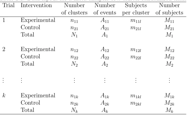
The data layout for a meta-analysis of k cluster randomized trials is provided in Table

2.1, where the notation used is defined in Table 2.2.

Suppose θ1, . . . , θk are the intervention effects of k trials, each measured as a log odds

ratio. Then the estimated intervention effect of θj of trial j is denoted

ˆ

θj =ln " ˆ

P1j(1−Pˆ2j)

ˆ

P2j(1−Pˆ1j) #

(31)

Table 2.1: Data layout for a meta-analysis of k cluster randomized trials.

Trial Intervention Number Number Subjects Number

of clusters of events per cluster of subjects

1 Experimental n11 A11 m11l M11

Control n21 A21 m21l M21

Total N1 A1 M1

2 Experimental n12 A12 m12l M12

Control n22 A22 m22l M22

Total N2 A2 M2

..

. ... ... ... ... ...

k Experimental n1k A1k m1kl M1k

Control n2k A2k m2kl M2k

Total Nk Ak Mk

Table 2.2: Notation used in Table 2.1 given that intervention groups i = 1,2, cluster

l = 1, . . . , nij and trial j = 1, . . . , k.

Symbol Description

mijl size of the ith group in cluster l of trial j

nij total number of clusters in group i of trial j

Nj =P2i=1nij total number of clusters in trial j

Mij =P

nij

l=1mijl total number of subjects in group i of trial j

Mj =P2i=1Mij total number of subjects in trial j

Aijl number of events of the ith group in cluster l of trial j

Aij =P

nij

l=1Aijl number of events in group i of trial j

Aj =P2i=1Aij total number of events in trial j

ˆ

Pijl =Aijl/mijl proportion of events of the ith group in cluster l of trial j

ˆ

(32)

2.3 Fixed effects model

A fixed effects model assumes that there is a common effect measure and a random

component (within study sampling error), which is responsible for observed between study

heterogeneity in a meta-analysis. The fixed effects model for the observed study-specific

intervention effect ˆθj is given (Whitehead, 2002) by

ˆ

θj =θ+j, (2.1)

where the sampling error j is assumed to be approximately independently and normally

distributed with mean 0 and within study variance σ_j2 and with overall mean effect sizeθ,

respectively, for trial j, j = 1, . . . , k.

2.3.1 Adjusted Q statistic

Individually randomized trials

The null hypothesis Ho for the Q statistic is given by θ1 = θ2 = . . . = θk = θ and the

alternative hypothesis HA is θi 6=θj for some i6=j. The mathematical expression for the

Q statistic is defined as a weighted sum of squares of the deviations of individual study

estimates from the overall mean effect size, given by

Q =

k X

j=1

ˆ

wj(ˆθj −θˆ)2 (2.2)

where the estimated overall mean effect size is given by

ˆ

θ =

Pk

j=1wˆjθˆj Pk

j=1wˆj

(33)

The estimated weights are the reciprocals of the estimated within study variances, given

by ˆwj = 1/σˆ2j. These particular weights are chosen to provide the most precise estimate

of θ by minimizing the variance of θ (Hardy and Thompson, 1996). Under Ho, the Q

statistic is distributed as a chi square random variable with k₋1 degrees of freedom.

The derivation of the Q statistic is provided in Appendix A.

In practice, the within study varianceσ2

j is estimated using data fromjth trial,j = 1, . . . , k.

Given the responses for the jth trial in Table 2.3,

Table 2.3: Responses for thejth trial

Positive Negative Total P(positive)

Experimental A1j M1j−A1j M1j P1j =A1j/M1j

Control A2j M2j−A2j M2j P2j =A2j/M2j

and applying Woolf (1955)’s approach to estimate the within study variance for the

estimated log odds ratio, denoted as ˆθj:

ˆ

wj = (ˆσj2)

−1 ₌ "

1

A1j

+ 1

M1j−A1j

+ 1

A2j

+ 1

M2j −A2j

#−1

=

"

1

M1jPˆ1j(1−Pˆ1j)

+ 1

M2jPˆ2j(1−Pˆ2j) #−1

.

Cluster randomized trials

In the case of cluster randomization trials where individuals of the same cluster are

correlated with a positive intracluster correlation coefficientρ, Donner and Donald (1987b)

suggested an adjustment using the variance inflation factor for each intervention group

i= 1,2 defined as

Cij =

nij

X

l=1

(34)

The intracluster correlation coefficient ρj may be obtained by using the ‘analysis of

variance’ (ANOVA) estimator proposed by Snedecor and Cochran (1980) (see Appendix

B for details). Consequently, the weights adjusting for clustering wjc become

ˆ

wjc = (ˆσjc2)

−1

=

"

C1j

M1jPˆ1j(1−Pˆ1j)

+ C2j

M2jPˆ2j(1−Pˆ2j) #−1

. (2.4)

Accordingly, replacing ˆwj in (2.2) by ˆwjc, the adjusted Q statistic is obtained by

Qa =

k X

j=1

ˆ

wjc(ˆθj −θˆc)2, (2.5)

where the estimated adjusted overall mean effect size is given by

ˆ

θc= Pk

j=1wˆjcθˆj Pk

j=1wˆjc

. (2.6)

The adjusted Q statistic asymptotically follows a chi square distribution with k ₋1

degrees of freedom under Ho (Song, 2004). Note that if ˆρj = 0 or Cij = 1 for i= 1,2 and

j = 1, . . . , k, indicating there is no clustering, ˆwjc reduces to ˆwj and Qa equals Q.

Now, the adjusted Q statistic from equation (2.5) may be rewritten as

Qa =

k X

j=1

ˆ

wjc(ˆθj −θ)2− k X

j=1

ˆ

wjc(ˆθc−θ)2 (2.7)

(35)

var(ˆθc) = Pk

j=1wˆjc2var(ˆθj)

Pk j=1wˆjc

2 = Pk

j=1wˆ2jcwˆ

−1 jc

Pk j=1wˆjc

2 =

1

Pk j=1wˆjc

. (2.8)

Assuming within study variances are known, the expectation of the adjusted Q statistic

under the null hypothesis based on equations (2.7) and (2.8) is given by

E[Qa|Ho] = k X

j=1

wjcE(ˆθj −θ)2− k X

j=1

wjcE(ˆθc−θ)2

=

k X

j=1

wjcvar(ˆθj)− k X

j=1

wjcvar(ˆθc)

=

k X

j=1

wjcw−jc1− k X j=1 wjc   k X j=1 wjc   −1

=k₋1.

2.3.2 Approximate power

Let δj denote the deviation of the intervention effectθj from the overall mean effect size

θ for trial j, j = 1, . . . , k, under the alternative hypothesis such that θi 6=θj for at least

one pair (i, j) or equivalently δj 6= 0 for at least one j (Montgomery, 2000, p.64). This

implies that the model in equation (2.1) for the observed intervention effect ˆθj becomes

ˆ

θj = θ+δj+j (2.9)

= θj+j,

since δj = θj −θ, where θ is the overall mean effect size. The sampling error j is

approximately normally distributed with mean 0 and within study varianceσ2

jc for trialj,

j = 1, . . . , k. The fixed effects δj has a constraint such that the sum of weighted δj equals

zero to satisfy the condition that ˆθc remains an unbiased estimator of θ with variance

of 1/Pk

(36)

because the expectation of j is equal to zero (i.e. E(j) = 0).

Next, replacing ˆθj defined in (2.7) by (2.9), the expectation of the adjusted Q under the

alternative hypothesis assuming the within study variance being known is given by

E[Qa|HA] = k X

j=1

wjcE(θ+δj+j −θ)2− k X

j=1

wjcvar(ˆθc)

=

k X

j=1

wjcE(δj2) + k X

j=1

wjcE(2j)−1

=

k X

j=1

wjc(θj−θ)2+k−1,

where the adjusted Q statistic is distributed as a noncentral chi square distribution with

k₋1 degrees of freedom and noncentrality parameter NC defined as

N C =

k X

j=1

wjc(θj−θ)2. (2.10)

The overall mean effect size θ may be estimated using ˆθc in equation (2.6). It follows that

the power of the adjusted Qstatistic at significance level α is defined as

power = 1₋P(Accept Ho|HA)

= 1₋P(Qa≤χ2k−1|HA)

= 1₋F(cα|k−1, N C), (2.11)

whereF(cα|k−1;N C) is the cumulative distribution function of the noncentral chi-square

with k₋1 degrees of freedom and noncentrality parameter NC given in equation (2.10)

(37)

2001).

In practice, parameters used for calculating statistical power are rarely available; therefore,

it is common to make some a priori assumptions. Based on these assumptions, we

investigate the approximate power of the adjusted Q statistic as a function of the number

of clusters, cluster size, disease risk rates, intracluster correlation coefficient and degree of

heterogeneity.

First, we focus on the case of an equal number of clusters n per intervention group,

where each cluster has a constant cluster size of m. Equal allocation is considered to be

statistically efficient as compared to unequal allocation, which requires more clusters to

obtain the same statistical power. In the case of unequal cluster sizes, we may replace m

by average cluster size ¯m. The slight underestimation of the actual sample size can be

negligible, providing that the variation in cluster size is not substantial. If m is replaced

by mmax, the statistical power calculated will be more conservative (Donner and Klar,

2000, p.57).

Second, for simplicity, we assume a constant within study variance across trials (i.e.

σ2

jc =σc2 for j = 1, . . . , k). However, in the case where the within study variance varies,

the noncentrality parameter assuming a constant within study variance tends to be

overestimated. Thus, the statistical power of the test obtained based on a constant within

study variance will be overestimated.

Third, Donner and Klar (2000, p.56) noted that the study design has an impact on the

es-timates of intracluster correlation coefficient. Since each of the trials in the meta-analysis

is assumed to be completely randomized, we will assume the intracluster correlation

(38)

Following these assumptions, the variance inflation factors defined in equation (2.3) are

reduced to 1 + (m₋1)ρ and the within study variance in (2.4) is simplified to a common

variance denoted byσ2

c, given by

σ_c2 = 1 + (m−1)ρ

nmP1(1−P1)

+ 1 + (m−1)ρ

nmP2(1−P2)

. (2.12)

Furthermore, the between study variance denoted byτ2

c (also referred to as the

heterogene-ity variance) can be estimated using the sample variance, given by Pk

j=1(θj−θ¯)2/(k−1),

where ¯θ =Pk

j=1θj/k. When the weights are assumed constant across trials, ¯θ is equivalent

to the overall mean effect size θc. Subsequently, Pkj=1(θj−θc)2 may be approximated by

(k₋1)τ2

c (Hedges and Pigott, 2001). Therefore, the noncentrality parameter in equation

(2.10) is approximated by

N C = (k₋1)τ_c2/σ2_c. (2.13)

Note that the ratio τ2

c/σ2c is a measure of the degree of heterogeneity (see section

5.3). However, for plotting purposes, τ_c2 and σ_c2 are considered as two separate

quan-tities. Therefore, without loss of generality, let the effect size (ES) be defined as

d= 2_|arcsin(P1)(1/2)−arcsin(P2)(1/2)|(Cohen, 1992), the values of disease rates (P1, P2)

corresponding to d= 0.20 (small effect size) and 0.50 (medium effect size) are (0.1,0.168)

and (0.1,0.293), respectively. The effect sizes are defined in term of the disease rates

in order to plot the power of the adjusted Q statistic in function of the between study

variance τ_c2 or the intracluster correlation coefficient ρ. Given the number of trials k,

number of clustersn, cluster sizem, disease rates (P1, P2), between study varianceτc2, and

intracluster correlation coefficient ρ, the power of the adjusted Q statistic was calculated

(39)

(P1, P2) = (0.1, 0.168), (0.1, 0.293)

(n, m) = (5, 50), (5, 100), (10, 50)

k = 5, 10, 20

τ_c2 = 0 to 0.5 in steps of 0.1

ρ = 0 to 0.05 in steps of 0.01

The values for the number of trialsk and between study variance τ2

c, are taken from Hardy

and Thompson (1998). Also, the values of the effect sizes and intracluster coefficients

in community intervention trials are frequently small (Donner and Klar, 1996). For

example, the intracluster correlation coefficients for four cluster randomization trials

(Jolly et al., 1999; Moher et al., 2001; Montgomery et al., 2000; Woodcock et al., 1999)

performed to compare two or more interventions in primary care for cardiovascular heart

disease (CHD), which will be used as an example for this research, were in the range

of 0 to 0.0125. Also, when the approximate power of the adjusted Q statistic plotted

against the between study variance τ2

c, the intracluster correlation coefficient ρ was set

to 0.01. But when the approximate power of the adjusted Q statistic plotted against

the intracluster correlation coefficientρ, the between study varianceτ2

c was then set to 0.1.

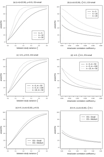
Figure 2.1(a)-(b) shows that the approximate power of the adjusted Q statistic increases

as the number of trials increases, while holding other variables constant. Similarly, in

Figure 2.1(c)-(d), the approximate power of the adjusted Q statistic increases as the total

sample size increases while holding other variables constant. In addition, for a given

total sample size (nm= 500), the adjusted Q statistic with n = 10 has greater power

than with n = 5. In Figure 2.1(e)-(f), the approximate power increases as the effect

size becomes larger while holding other variables constant because larger effect size with

largerP2(1−P2) in equation (2.12) givenP1 fixed results in smaller constant within study

variance. From the plots of power againstτ2

c (first column), it is seen that the approximate

power increases as τ_c2 increases. For instance, in Figure 2.1(a), the approximate power of

the adjusted Q statistic is approximately 60% for τ2

c = 0.2 and 80% for τc2 = 0.4 while

(40)

of power against ρ (second column), it is seen that the approximate power decreases

as ρ increases. For instance, in Figure 2.1(b), the approximate power of the adjusted

Q statistic is approximately 80% for ρ = 0 and 40% for ρ = 0.02 while fixing k = 10,

(n, m) = (5,50), τ2

c = 0.1, andES =small.

2.4 Summary

In summary, since the validity of the unadjusted Q statistic in the presence of clustering

becomes questionable with inflated Type I error rates, the adjusted Q statistic has been

introduced. In addition, the approximate power of the adjusted Q statistic was derived

from a noncentral chi square distribution with k₋1 degrees of freedom and a specified

noncentrality parameter.

We have also investigated the power in terms of parameters including the number of

trials, number of clusters, cluster size, disease rates between intervention groups (i.e.

effect size), between study variance and intracluster correlation coefficient. It appears

that the power of the adjusted Q statistic increases by increasing any of the following

parameters: number of trials, overall sample size per trial (i.e. n_×m), effect size (disease

rates between intervention groups) and between study variance. In contrast, the power

decreases as the intracluster correlation coefficient increases. Moreover, for a fixed sample

size, it is seen that the power of the adjusted Q statistic is greater for a large number of

(41)

(a) (n,m)=(5,50), ρ=0.01, ES=small

between study variance τc 2

po

w

er(%)

k=5 k=10 k=20 0 20 40 60 80 100

0.0 0.1 0.2 0.3 0.4 0.5

(b) (n,m)=(5,50), τc 2

=0.1, ES=small

intracluster correlation coefficient ρ

po

w

er(%)

k=5 k=10 k=20

0 20 40 60 80 100

0.000 0.010 0.020 0.030 0.040 0.050

(c) k=5, ρ=0.01, ES=small

po

w

er(%)

n=5, m=50 n=5, m=100 n=10, m=50 0 20 40 60 80 100

0.0 0.1 0.2 0.3 0.4 0.5

(d) k=5, τc 2

=0.1, ES=small

po

w

er(%)

n=5, m=50 n=5, m=100 n=10, m=50

0 20 40 60 80 100

0.000 0.010 0.020 0.030 0.040 0.050

(e) k=5, (n,m)=(5,50), ρ=0.01

po

w

er(%)

ES=Small ES=Medium 0 20 40 60 80 100

0.0 0.1 0.2 0.3 0.4 0.5

(f) k=5, (n,m)=(5,50), τc 2

=0.1

po

w

er(%)

ES=Small ES=Medium

0 20 40 60 80 100

0.00 0.01 0.02 0.03 0.04 0.05

Figure 2.1: Approximate power of Qa plotted against τc2 (first column) and ρ (second

column). (a)-(b) varying numbers of trials k (k = 5,10,20); (c)-(d) varying number of

clusters per trial n and cluster size m ((n, m) = (5,50),(5,100),(10,50)); (e)-(f) varying

(42)

Chapter 3 Heterogeneity variance estimation

3.1 Introduction

The fixed effects model described in Chapter 2 assumes homogeneity of intervention effects

across the k trials. In contrast, the random effects model assumes that the observed

trials are a random sample from a hypothetical population of trials. In order to account

for the variation among trials, a random term known as heterogeneity variance is added

to compute the weights in the random effects model; this tends to equalize the weights

assigned to small and large trials. Subsequently, the random effects model may lead to

wider confidence intervals for the overall intervention effect.

Heterogeneity variance is also used as a measure of heterogeneity in meta-analysis.

Al-though heterogeneity variance may be solely limited to trials with the same effect measures

(e.g. odds ratio, risk ratio and hazard ratio), its value does not depend on the number, or

size of trials in a meta-analysis unlike the other measures such as the Q statistic (R¨ucker

et al., 2008).

The aim of this chapter is to extend existing approaches for estimating the heterogeneity

(43)

randomization trials. We begin by considering eight methods for estimating the

hetero-geneity variance. In addition to a point estimate, confidence intervals for the heterohetero-geneity

variance estimate may be useful, as they indicate its precision while also conveying all the

information contained in the corresponding test of heterogeneity (Hardy and Thompson,

1996; Viechtbauer, 2007a). Moreover, such confidence intervals may be also used to

construct confidence intervals for measures of heterogeneity (Higgins and Thompson,

2002), which will be discussed in Chapter 4.

The random effects model for cluster randomization trials is briefly described in Section

3.2. The eight approaches for estimating the heterogeneity variance adjusted for clustering

and the six methods for constructing confidence intervals, which are introduced in Section

1.2.3, are discussed with corresponding mathematical expressions presented in Section 3.3

and 3.4, respectively. Furthermore, a simulation study conducted in order to assess the

bias and mean square error of the adjusted heterogeneity estimators and the coverage

probabilities of the confidence intervals appears in Chapter 5.

3.2 Random effects model

Let ˆθj denote the estimated intervention effect (experimental vs. control) on the log

odds ratio of the study outcome for the jth trial, j = 1, . . . , k. The random effects

meta-analysis model (Whitehead, 2002, p.88) is given by

ˆ

θj =θ+νj+j,

where θ is the true overall mean effect size. Also, two independent random effects

in-cluded in the model are the random study effects and the error terms, denoted by νj and

j, respectively. Random study effects are assumed to be independently and normally

(44)

are assumed to be independently and normally distributed with mean 0 and variance σ2 jc,

(i.e. j ∼N(0, σ2jc)), whereτc2 is the between study component of variance also known as

the heterogeneity variance andσ2

jc is the within study component.

In practice, the within study variance is estimated using equation (2.4) for cluster

ran-domization trials ignoring the sampling errors within the trial. This practice is often used

because the within study variance tends to be relatively small as compared to the between

study variance. Therefore, the errors can be negligible. However, caution must be taken

using the estimated within study variance as the true variance for trials with small overall

sizes, where the large sample approximation may be questionable (Bohning et al., 2002;

Brockwell and Gordon, 2001; Sidik and Jonkman, 2006). In this chapter, the focus will

be restricted to estimating heterogeneity varianceτ2

c, with σjc2 being assumed known.

3.3 Adjusted heterogeneity variance estimators

τ

_c2

3.3.1 Variance component estimator (VC)

Hedges and Olkin (1985) proposed a simple approach to estimate the heterogeneity

variance using a method similar to that for estimating the variance components in a

random effects analysis of variance. Given the unweighted mean ¯θ= Pk

j=1θˆj/k, the usual

sample variance of ˆθj may be expressed as

S_θ2 = 1

k₋1

k X

j=1

(ˆθj−θ¯)2.

Then the expected value of S2

θ in terms of variance components is

E[S_θ2] =τ_c2+ 1

k

k X

j=1

ˆ