Diagnosis of the Best Method for Wind Speed
Extrapolation
Dr. Firas A. Hadi
Department of Wind Energy, Ministry of Science and Technology, Baghdad, Iraq
ABSTRACT: The standard height of meteorological towers for wind speed observations is 10 meters. Since wind turbine hub heights are typically more than thisheight, extrapolation of wind speeds to the planned hub height is usually required, the most elementary models for predicting the adjusted wind speed are power law and logarithmic law.The purpose of this paper is to extrapolate the wind speed and power density to different heightsusingpowerlaw, logarithmic law,and wind speed distribution extrapolation;thenthe results werecompared with the real data taken from sensors located atdifferentheightsfor the purpose of knowing the best representation method. The sensors are installed at 10, 30, 52 meters heights from ground surface at Al-Shehabi site in Iraq. Also, for more benefits, both of results and the observed data (real data) were compared with wind resource map of Iraq (Geosun) in order to know the accuracy of map’s data. It is found that the wind speed distribution extrapolationgives more acceptable results than the power and logarithmic lawsfor extrapolation procedure, at the same time it was proved that how much extent the validity of map is.
KEYWORDS: Extrapolation, Power law, Log law, Distribution Extrapolation.
Nomenclature
Abbreviations
WT wind turbine PL power law LogL logarithmic law
LIDAR light detection and ranging SODAR Sonic detection and ranging
Variables
v1 wind speed at reference height (m/sec)
v2 wind speed at another height (m/sec) z0 roughness length (m)
z1 roughness length at reference height z2 roughness length at another height
ρ density of the air
Zo1 is roughness length at reference location Zo2 is roughness length at destination location n Weibull distribution extrapolation exponent α or Alpha Hellman’s wind shear exponent z elevation above the ground
ĸvon Karman constant
u∗friction velocity
τ surface value of the shear
h1 wind speed at a reference height
h2 wind speed at another height (hub height) c1 Weibull scale factor at h1 height
k1 Weibull shape factor at h1 height c2 Weibull scale factor at h2 height k2 Weibull scale factor at h2 height
I. INTRODUCTION
Wind measurements are generally performed below WT hub heights owing to the higher measurement and tower cost. Therefore, a wind shear model proves to be necessary to extrapolate the observed wind resource from the available lower heights to the wind turbine hub height, [1].
ofyear, and from one year to the other. Thus, wind speedextrapolation might be regarded as one of the most critical uncertainty factor affecting wind power assessment, particularlywhen considering the increasing size of modern wind turbines. Actually, critical errors between estimated and actual energyoutput may result from application of this extrapolation, and the use of devices such as LIDARor SODAR to eliminate errors due to shear model uncertainty largely increase the costs of a wind powerproject, often making it economically not viable, while increasingknowledge on wind shear models to strengthen their reliabilityappears as preferable, [1].
In this study a validity of each power law, logarithmic law, speed distribution, and Geosun map is achieved after a comparison with the real data, this will show us the most applicable one at Al-Shehabi site.
AREA OF STUDY
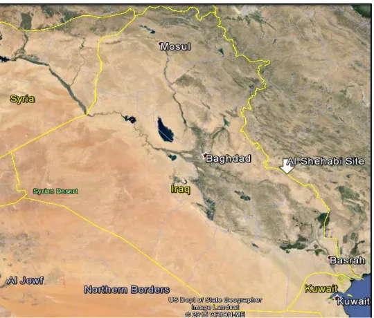
The feasibility and applicability of wind energy development depends on the physical characteristics of the study area and the wind resource. The region is located in the area between Maysan and Wasit. It is 112 km from Maysan, 85 km from Wasit, and about 220 km from Baghdad at position 32.77°N 46.70°E; Figure. 1 shows the location of chosen site in eastern region near the border between Iraq and Iran.
Fig. 1Iraq satellite image to indicate the area of study
II. BACKGROUND
Since methods and models applied in the current work are the same as in the previous one, the reader should refer to the corresponding Background section[2], where the following are presented: (i) the PL by Hellman derived equation to calculate alpha base don record so fv1 and v2;(ii) the Log L, and derived equation to assess z0 underneutra lstability conditions; (iii) models forestimating alpha such as Smedmane Högström and Högström[3], and(iv) models forest imatingn such as Just us and Mikhail[4].
III. GEOSUN MAP
Wind View allows users to view and query wind data in an interactive environment, as well as modifies, copy, and print maps. With the selected methodology it is possible to obtain virtual hourly datasets at any specified position and any height above ground level.
IV. LOGARITHMIC LAW
The logarithmic law origins lie in the boundary layer fluid mechanics and atmospheric research. To determine the horizontal velocity (v) at a height (z), it is commonly expressed as follows:
( ) = ( ∗
ĸ) ln( ) (1) Where ĸ =0.4 is von Karman constant. (u∗= ). The roughness length( ) describes the roughness of the ground
or terrain where the wind is blowing. There are cases where wind velocity v1is known and required at anotherheight( ) in a case that can be derived from Eq.1 [5]:
= ( )− ( )
( )− ( ) (2)
It is a simple expression to solve, as it eliminates the need to calculate the friction velocity and von Karman constant, which could be difficult to estimate in the atmosphere. A neutral wind profile is assumed, where convection is negligible, the lapse rate (the fall of temperature in the troposphere with height) is nearly adiabatic.
Note that Eq.2gives estimation on the speed at one location. In case one wants to compare two locations (for example, meteorological station and wind turbine site), each with its own roughness length with similar wind profile, thenWieringa'sassumption that the wind speed at 60m height is unaffected by the roughness, leads to the formula, [6]:
( ) ( )=
° ( ⁄ ° )
° ( ⁄ ° )
(3)
V. POWER LAW
The power law equation is a simple, yet useful model of the vertical wind profile which was first proposed by Hellman (1916). The power law profile assumes that the ratio of wind speeds at different heights can be found by the following equation:
= ℎ
ℎ (4)
The shear exponent α (Alpha) can be directly measured once records of v1 and v2 are available:
= ℎ
ℎ
(5)
(a) Log law (b) power law
Fig.2Example wind shear profiles using Log law and power law models
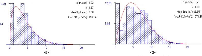
If the winds hear coefficient, α, cannot be determined correctly, the difference between the predicted and observed wind energy production might be upto 40%,due to turbulence effects, time interval of wind data measurement, and the extrapolation of the data from reference height to hubheights. In the literature, the winds hear coefficientis a highly variable quantity, often changing from less than 0.14 during the day to more than 0.5 at night over the same terrain. Also, wind shear coefficient was measured to typically range from 0.40 in urban areas with high buildings to 0.10 over smooth, hard ground, lakes or ocean However, in real situations, a winds hear coefficient is not constant and depends on numerous factors, including atmospheric conditions, temperature, pressure, humidity, time of day, seasons of the year, the mean wind speed, direction, and nature of terrain, Table1 demonstrates the various winds hear coefficients for different type softopography and geography, [1].
Table 1: Shear exponent values according different Terrain Type
From Eq. (4), α can be directly measured once records of v1 and v2 are available:
VI. THE WEIBULL WIND SPEED DISTRIBUTION EXTRAPOLATION
Justus and Mikhail suggested a useful full range of wind speed, as required to specify the wind speed probability distribution. They demonstrated the power law relationship between wind profiles Eq.4 to be consistent with the height variation of the Weibull wind speed distribution, at least under the assumption of heights below 100m and a fairly level terrain (though over a wide range of roughness length)[8]. Thus, if Weibull probability distribution at reference height h1 is p(v1), then p(v2) at any other height h2 may be derived. In other words, if c1 and k1 Weibull functions are known at. Some anemometer height h1, then the values of c2 and k2 at any desired height h2 (e.g., the turbinehubheight)canbeassessedby:
= ℎ
ℎ (6)
Terrain Type value
Lake, ocean, and smooth hard ground 0.1
Foot-high grass on level ground 0.15
Tall crops, hedges, and shrubs 0.2
Wooded country with many trees 0.25
Small town with some trees and shrubs 0.3
= 1−0.0881 ln(ℎ /ℎ )
1−0.0881 ln(ℎ /ℎ ) (7)
Where ℎ a reference height of 10m and the exponent n is was empirically found to be:
= 0.37−0.0881 ln( )
1−0.0881 ln(ℎ /ℎ ) (8)
Note that for n a different notation from a commonly used to emphasize its different meaning, although the and n
strict relationship has been experimentally demonstrated by [9]. He also pointed out that, while depends on several surface properties, n only depends on c and h of the measurement height.
VII. RESULTS AND DISCUSSIONS
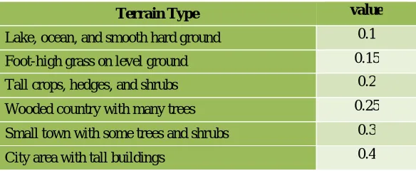
The histograms for Al-Shehabi site at 10m and 52m heights are shown in Fig.3 below, where most of the wind speedsare concentrated under 5m/sec from the distribution (Fig.3-a), such that 69% from the spectrum is represented below of this number, and 18.7% from the distribution is recorded in 3-4 interval (excluded 0-1). While the distribution is slid toward high value portion (Fig3-b) such that 41%from the spectrum is represented below 5m/sec, and 10.7% from the distribution is recorded in 3-4 interval (excluded 0-1). Weibull probability density function representation of the histogram are shown in red curves in Fig.3. These two shapes will form the basis for the subsequent calculations.
-a- -b-
Fig. 3Histogram and Weibull distribution for Al-Shehabi site at (a) 10m and (b)52m height
The Power law and the Logarithmic law are the two most commonly used analytical models for extrapolating wind speeds to higher heights. The results of these two laws are shown in Figs. 4 and 5. Fig.4 represents the extrapolation of wind speed data using Logarithmic law, 1st column in this figure is founded using Eq.2, while 2nd column is founded using Eq.3. Fig4.a and Fig4.c represent the extrapolation from 10m to 52m height, Fig4.b and Fig4.d represent the extrapolation from 52m to 100m height. Weibull probability density function is plotted as continues red curves for the purpose of data representation.
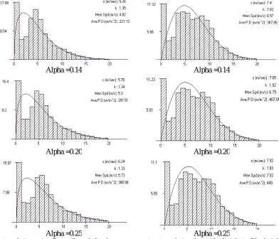
Fig.5represents the results of extrapolation using Power law, left column represents extrapolation from 10m height to 52m,whereas right column represents extrapolation from 52m height to 100m height at different wind shear exponent (Alpha) values 0.14, 0.2, and 0.25. These values have been selected on the basis that the standard is 0.14 and 0.25 value calculated from equation5, while 0.2 value has been selected arbitrarily and as a value lies between two previous values.
Alpha =0.14 Alpha =0.14
Alpha =0.20 Alpha =0.20
Alpha =0.25 Alpha =0.25
Fig. 5Extrapolation using Power Law, left column represents extrapolation from 10m height to 52m height, right column represent extrapolation from 52m height to 100m height
The results derived from Figs. 3, 4, and 5 can be collected in the Table2 shown below.
d- extrapolation 52 to 100 (log site-turbine law) b- extrapolation 52m height to 100m height
Table 2: Results Summary extrapolation of wind speed from 10 to 52 and from 52 to 100
Now, by applying equations 6 and 7 the wind speed distribution could be rise from 10m to 52m, the results is summarized in Table 3 below.
Table 3: Results of Weibull distribution extrapolation
The 2st column in Table 2 gives the data taken from Geosun map; 3th and 4th columns show the extrapolated wind data from 10m height to 52m height by applying Logarithmic law (Eq.2) at roughness length equal to 0.0024. While 5nd,6rd, and 7th columns in Table 2 give the extrapolated wind data from 10m height to 52m height by applying Power law (Eq.4) at alpha equal to 0.14, 0.2, and 0.25 respectively.
From Table 2 it can be concluded that the Power law gives better results than logarithmic law. This can be seen throughout the comparison between the wind speed and power density values that observed at a 52m height (taken from meteorological tower located at Al-Shehabi site) and data that calculated from Power law in order to extrapolate mean wind speed and power density from 10m to 52m height. The minimum difference between actual wind speed at 52m (5.59 m/s) and calculated one (5.7 m/s) is noticed at alpha equal to 0.25, while the minimum difference between actual power density at 52m (274 w/m2) and calculated one (297 w/m2) is noticed at alpha equal to 0.2.
Now, by a comparison between the above results of mean wind speed (5.95 m/s) and power density (274 w/m2) with the results exist in Table3 (mean wind speed 5.6 and power density 274 w/m2), it could infer that the distribution extrapolation gives more suitable results than that by using Power and Logarithmic laws.
From Fig.6 it could be easily seen the extent of convergence between the observed data (field data) and the results extracted from the process of probability distribution extrapolation.
ExtrapolationMethod Geosun
Log(site-turbine) law (z0=0.0024) Log law (z0=0.0024) Power law (alpha=0.14) Power law (alpha=0.2) Power law (alpha=0.25)
Using Eq. 5
Actual from tower at52m Avg. wind speed at
52m 5.2 m/s 4.61 m/s 4.61 m/s 4.82 m/s 5.3 m/s 5.7 m/s 5.95m/s
P.D. at 52m 246
w/m2 190 w/m
2
190 w/m2 221 w/m2 297 w/m2 380 w/m2 274w/m2
C at 52m 6.61
m/s 5.03 m/s 5.03 m/s 5.26 m/s 5.78 m/s 6.24 m/s 6.7m/s
K at 52m 1.80 1.36 1.36 1.35 1.34 1.33 1.81
Actual at 52m
Extrapolated values 10m to 52m
Extrapolated values 10m to 100m
Geosun 100m
C(m/s)at 52m 6.7 m/s 6.3 m/s 7.38 m/s 7.30
K at 52m 1.81 1.6 1.71 1.73
Mean wind speed
(m/s) 5.9 5.6 6.6 6.5
Fig.6Comparison between all previous results,Pdf extrapolation is butter way
VIII. CONCLUSION
From the above discussion it could be concluded that:-
1- In case of data availability at a certain height and not available at a higher altitude than the previous, it is possible to use the extrapolation of wind speed or using the extrapolation of probability distribution.
2- It is possible to make wind speed extrapolation by mathematical laws such as Power law or Logarithmic law. 3- Power law gives more adequate results than logarithmic law.
4- Wind shear exponent (Alpha) is very important parameter in determining the accuracy of extrapolation. In another hand the determining of Alpha value by mathematical equation gives closer value to reality than the standard values.
5- The power law is widely used due to its simplicity, and it seems to give a better fit to most of the data over a greater height range and for higher wind conditions, compared to the log logarithmic law.
6- The results indicated that the process of distribution extrapolation gives more better results and more accurate than the using of mathematical laws.
REFERENCES
1. Giovanni Gualtieri, SauroSecci"Extrapolating wind speed time series vs. Weibull distribution to assess wind resource to the turbine hub height: A case study on coastal location in Southern Italy",Renewable Energy vol.62, (2014),pp 164-176
2. Gualtieri G., Secci S. “Methods to extrapolate wind resource to the turbine hub height based on power law” a1eh wind speed vs. Weibull distribution extrapolation comparison. Renewable Energy 2012, Vol. 43, pp183-200.
3. Smedmane Högström A S, Högström U. “A practical method for determining Wind frequency distributions for the lowest 200m from routine meteorological data”, Journal of Applied Meteorology 1978; Val.17,pp942-954.
4. Justus C.G., Mikhail A., “Height variation of wind speed and wind distributions statistics”, Geophysical Research Letters 1976; Vol.3, Issue 5,pp 261-264.
5. [5] Spera D.A., Richards T.R.,“Modified power law equations for vertical wind profiles”, Conference and work shop on wind energy characteristics and wind energy siting, Portland, OR, USA, June1979, pp.19-21.
6. Firas A. H., “Constructionof Mathematical-Statistical Model ofWind Energy in Iraq Using DifferentWeibull Distribution Functions”, Ph.D. Thesis, AL-Nahrain University, College of Science, Department of Physics, 2014.
7. Basim A. Alknani, “Effects of Turbulence Intensity on Wind Turbine Performance”, Ph.D. Thesis, Al-Mustansiriya University, College of Science, Department of Atmospheric Sciences, 2014.
8. Sunday O. O., Adaramola M. S., and Paul S. S., "Analysis of Wind Speed Data and Wind Energy Potential in Three Selected Locations in South-East Nigeria", International Journal of Energy and Environmental Engineering, 3:7, 2012.