Western University Western University
Scholarship@Western
Scholarship@Western
Electronic Thesis and Dissertation Repository
4-22-2013 12:00 AM
Comparison of option pricing between ARMA-GARCH and
Comparison of option pricing between ARMA-GARCH and
GARCH-M models
GARCH-M models
Yi Xi
The University of Western Ontario Supervisor
Dr. Reginald J. Kulperger
The University of Western Ontario
Graduate Program in Statistics and Actuarial Sciences
A thesis submitted in partial fulfillment of the requirements for the degree in Master of Science © Yi Xi 2013
Follow this and additional works at: https://ir.lib.uwo.ca/etd
Part of the Other Statistics and Probability Commons
Recommended Citation Recommended Citation
Xi, Yi, "Comparison of option pricing between ARMA-GARCH and GARCH-M models" (2013). Electronic Thesis and Dissertation Repository. 1215.
https://ir.lib.uwo.ca/etd/1215
This Dissertation/Thesis is brought to you for free and open access by Scholarship@Western. It has been accepted for inclusion in Electronic Thesis and Dissertation Repository by an authorized administrator of
COMPARISON OF OPTION PRICING BETWEEN ARMA-GARCH AND
GARCH-M MODELS
(Thesis format: Monograph)
by
Yi Xi
Graduate Program in Statistics and Actuarial Science
A thesis submitted in partial fulfillment
of the requirements for the degree of
Master of Science
The School of Graduate and Postdoctoral Studies
The University of Western Ontario
London, Ontario, Canada
c
Abstract
Option pricing is a major area in financial modeling. Option pricing is sometimes based on normal GARCH models. Normal GARCH models fail to capture the skewness and the leptokurtosis in financial data. The variant GARCH-in-mean (GARCH-M) model is widely used in the option pricing literature. It adds a heteroskedasticity term to the mean equation, which is interpreted as a risk premium, and also incorporates a type of asymmetry.
Our goal is to compare option valuation between GARCH-M and ARMA-GARCH models with normal and non-normal,z-distributed innovations. The models are fitted to the historical return data, and risk neutral measures are based on the conditional Esscher transform and the extended Girsanov principle. We compare European Calls on the S&P 500 with the model predictions. The TGARCH is best for ARMA-GARCH/GARCH-M models. Neither normal nor z dominates the other, but overallz-TGARCH-M (z-innovations) seems to be best, ARMA-TGARCH is surprisingly good.
Keywords: option pricing, ARMA-GARCH, GARCH-in-Mean, z-distribution, Esscher transform, Extended Girsanov principle
Acknowlegements
First and foremost, I would like to express my deepest gratitude to my program supervisor Dr. Reginald J. Kulperger for his generous support, encouragement, patience and valuable guidance during my time at University of Western Ontario. During these two years spent at Western he was not only my academic supervisor but also my mentor. I deeply indebted to you for all that you have done for me during all these years.
I was one of recipients of Richard Konrad Ontario Graduate Scholarship. I really appreci-ated the generous support from Mr. Konrad and the Provincial Government.
I also wish to express my heart-felt thank you to all the faculty, staff, and fellow graduate students in the Department of Statistical and Actuarial Science who have made my stay here both enjoyable and memorable.
My sincere thanks to Dr. Mark Resser, Dr. Matt Davison and Dr. Rogemar Mamon for agreeing to act as examiners.
I am appreciated the selfless love, devotion, and encouragement from my parents. In addi-tion, I am grateful to my husband Lijun. Her love, support and words of encouragement have been a constant that I have been able to count on throughout this experience.
Contents
Abstract ii
Acknowlegements iii
List of Figures vii
List of Tables viii
List of Appendices x
1 Introduction 1
2 Financial Series and Models 4
2.1 Financial Time Series . . . 4
2.2 ARMA Model . . . 5
2.3 GARCH Model . . . 6
2.3.1 Properties of the GARCH(1,1) Models . . . 7
2.3.2 Extensions of GARCH Model . . . 8
3 Estimation of the GARCH Models 11 3.1 Estimation Methods . . . 11
3.1.1 Maximum Likelihood Estimation . . . 11
3.1.2 Quasi-Maximum Likelihood . . . 12
3.2 Estimating ARMA-GARCH and GARCH-M Models . . . 14
3.3 Model Fitting Analysis . . . 16
4 Risk Neutral Measures Under GARCH Models 22 4.1 Definitions and Notations . . . 22
4.2 Risk Neutral Measures . . . 24
4.2.1 Conditional Esscher Transform . . . 24
4.2.2 Extended Girsanov Principle . . . 26
4.3 Applications for GARCH Models . . . 27
4.3.1 GARCH with Normal Innovation . . . 27
4.3.2 GARCH withZ-distributed Innovation . . . 28
5 Numerical Experiments 32 5.1 Simulation Steps . . . 32
5.2 Option Data Description . . . 34
5.3 Empirical Analysis . . . 37
5.3.1 Option Data Set 1 . . . 37
5.3.2 Option Data Set 2 . . . 46
6 Conclusion and Future research 52 6.1 Conclusion . . . 52
6.2 Future Research . . . 53
Bibliography 55
A Tables of Pricing Errors for Example 2 59
Curriculum Vitae 68
List of Figures
3.1 Daily closing prices and returns of S&P 500 Index from January 02, 1988 to January 06, 2004 . . . 17 3.2 Log-density of observed residuals versus their theoretical density for Normal
distribution . . . 20 3.3 Log-density of observed residuals versus their theoretical density forz-distribution
21
5.1 European Call option price evaluated on April 18, 2002 for different models with the maturitiesT = 22, 46, 109, 173, and 234 days; the closing stock price on that day wasS0= $1124.47. . . 40
5.1 Continued Table: European Call option price evaluated on April 18, 2002 for different models with the maturitiesT = 22, 46, 109, 173, and 234 days; the closing stock price on that day wasS0= $1124.47. . . 41
5.2 Model pricing errors for European Call options on April 18, 2002. . . 42 5.2 Continued Table: Model pricing errors for European Call options on April 18,
2002. . . 43 5.3 Implied volatility smiles based on MLE estimates using returns from January
07, 2004 to December 29, 2004 . . . 49
List of Tables
3.1 ϵ˜t(ϑ) and ˜σt2(ψ) in GARCH models . . . 15
3.2 GARCH and TGARCH parameters estimated by MLE with normal innovations using daily closing prices of S&P 500 from January 02,1988 to January 06, 2004 18 3.3 GARCH and TGARCH parameters estimated by MLE, which under the
as-sumption onz-distributed noise, using daily closing prices of S&P 500 from January 02, 1988 to January 06, 2004 . . . 19
5.1 S&P 500 call option prices from Schoutens (2003) . . . 35 5.2 Number of Call option contracts (S&P 500 Index, January 07, 2004 to
Decem-ber 29, 2004 ) . . . 36 5.3 Average price of Call option contracts (S&P 500 Index, January 07, 2004 to
December 29, 2004 ) . . . 36 5.4 Overall pricing errors for European Call options on April 18, 2002 . . . 38 5.5 GARCH and TGARCH parameters estimated by MLE with normal distribution
using daily closing prices of S&P 500 from January 02, 1988 to April 17, 2002 44 5.6 GARCH and TGARCH parameters estimated by MLE, which under the
as-sumption onz-distributed noise, using daily closing prices of S&P 500 from January 02, 1988 to April 17, 2002 . . . 45 5.7 Overall pricing errors for European Call options in data set 2 . . . 46 5.8 Overall pricing errors regarding to moneyness(Call option contracts of S&P
500 Index, January 07, 2004 to December 29, 2004) . . . 50 5.9 Overall pricing errors regarding to maturity (Call option contracts of S&P 500
Index, January 07, 2004 to December 29, 2004) . . . 51
A.1 Pricing errors for GARCH-M (Call option contracts of S&P 500 Index, January 07, 2004 to December 29, 2004) . . . 60 A.2 Pricing errors for TGARCH-M (Call option contracts of S&P 500 Index,
Jan-uary 07, 2004 to December 29, 2004) . . . 61 A.3 Pricing errors for ARMA-GARCH (Call option contracts of S&P 500 Index,
January 07, 2004 to December 29, 2004) . . . 62 A.4 Pricing errors for ARMA-TGARCH (Call option contracts of S&P 500 Index,
January 07, 2004 to December 29, 2004) . . . 63 A.5 Pricing errors for z-GARCH-M (Call option contracts of S&P 500 Index,
Jan-uary 07, 2004 to December 29, 2004) . . . 64 A.6 Pricing errors for z-TGARCH-M (Call option contracts of S&P 500 Index,
January 07, 2004 to December 29, 2004) . . . 65
A.7 Pricing errors for z-ARMA-GARCH (Call option contracts of S&P 500 Index, January 07, 2004 to December 29, 2004) . . . 66 A.8 Pricing errors for z-ARMA-TGARCH (Call option contracts of S&P 500
In-dex, January 07, 2004 to December 29, 2004) . . . 67
List of Appendices
Appendix A Tables of Pricing Errors for Example 2 . . . 59
Chapter 1
Introduction
The theory of option pricing is an important topic in the financial literature. The seminal works of Black and Scholes and Merton were the starting point for European option pricing. Follow-ing the findFollow-ing that these model prices systematically differ from market prices, the literature on option valuation has formulated a number of theoretical models designed to capture these empirical biases. Many empirical studies on asset price dynamics have demonstrated that char-acteristics such as time-varying volatility, volatility clustering, non-normality, and leverage effect etc. should be taken into account when modelling financial data. Therefore various mod-els and techniques were developed in both discrete and continuous time to incorporate some or all of the above properties.
The significant contribution in the continuous-time financial literature includes the stochas-tic volatility models (Wiggings [Wig87], Hull and White [HW87], Scott [Sco87], Stein and Stein [SS91], Heston [Hes93]), jump-diffusion models (Bates [Bat96], Bakshiet al. [BCC97], and Scott [Sco97]) and models with jumps in both the asset price and volatility (Duffieet al.
[DPS00] and Chernov et al. [CGGT03]). More recently, Carr et al.[CGMY03] investigated the option pricing performance of a time-changed L´evy process. Although the continuous time models hold advantages in constructing closed form solutions for European option prices, their Markovian structure is not consistent with the empirical findings. In practice they are difficult to implement and test.
The discrete time literature has been dominated by the class of autoregressive conditional heteroscedastic models (ARCH) introduced by Engle [Eng82] or its generalization (GARCH) as first defined by Borellslev [Bor86]. The main advantage of these models stands in the relative ease of estimation. Thus, in the last few years, much interest has given to GARCH option price. However, simple GARCH specifications can capture only some of the skewness and excess kurtosis found in financial data, and this has led to the developments of a large number of extensions, all trying to give a better description of the data.
The first important extension was to investigate return process for GARCH models with non-normal innovations. Excess kurtosis can be taken account for by the heavier-tailed distri-butions such as Students t (Bollerslev [Bor87]) or the GED distribution (Nelson [Nel91]), but these were unable to explain excess skewness. Asymmetry can be incorporated using leverage effects (Nelson [Nel91] and Glostenet al. [GJ93]), or by assuming skewed innovation densi-ties such as normal inverse Gaussian distribution (Forsberg and Bollerslev [FB02]) and inverse Gaussian density (Christoffersen et al. [CHJ06]). Various any other parametric distributions
2 Chapter1. Introduction
are also implemented in a GARCH framework: Shifted Gamma (Siuet al. [ST04]), General-ized Error (Duan [Dua99]), α−stable (Menn and Rachev [MR05]), Normal Inverse Gaussian (Stentoft [Ste06]), mixture of normals (Badescuet al. [BKL08]), Poisson-normal innovations (Duanet al. [DRS06]) and thez-distribution (Lanne and Saikkonen [LS05]).
A second important issue addressed in the GARCH option pricing literature is the impact of different volatility specifications. Replacing standard GARCH model with asymmetric ones such as exponential GARCH or threshold GARCH, is another extension. Hardle and Hafner [HH00] proposed a model relying on the Glostenet al. [GJ93] asymmetric volatility process, called the GJR model, while Christofferson and Jacobs [CJ04] argued that a simple leverage effect in the conditional variance process outperforms most of the extensions considered in the literature relative to option prices.
It is well known that in the GARCH setup markets are incomplete, so there exist contingent claims which cannot be replicated exactly by constructing a self-financing hedge. Therefore there is an infinite number of risk neutral measures under which one can price derivatives. Option pricing in GARCH models has been typically done using the local risk neutral valuation relationship (LRNVR) pioneered by Duan [Dua95], but his method depends very strongly on the Gaussian innovations’ distribution. Since this method does not apply when relaxing the conditional normality assumption of the asset returns, researchers try to exploit other possible choices for the pricing kernels. Follmer and Schweizer [FS91] constructed minimal martingale measure (MMM), which is consistent with common criteria to find strategies that minimize cost process. Elliott and Madan [EM98] introduced an extended Girsanov principle (EGP) to construct a risk neutral measure which is supported by finding similar hedging strategies. A well-known tool in actuarial science is the Esscher transform. It was introduced in the option pricing literature by Gerber and Shiu [GS94]. Another martingale measure is a mean correcting martingale measure (MCMM) driven by geometric L´evy processes (Schoutens [Sch03]).
GARCH-type models used for option pricing are usually GARCH-M models; see for ex-ample Duan [Dua95] for normal innovation or Badescu [Bad07] for non-normal innovation. GARCH-M models include a risk premium as proposed by Engle, Lilien and Robins [ELR87]. The main motivation of this thesis is to test the necessity of the risk premium within the re-turn process for option pricing. Thus, we compare the option pricing performance between the widely used GARCH-M and ARMA-GARCH models. If an ARMA-GARCH model predicts option prices as well as a GARCH-M model it raises questions about the interpretation of the risk premium parameter for the GARCH-M.
Another motivation for this comparison stands on the model’s simplicity and understand-ability. The estimation theory of ARMA-GARCH models provided by QMLE and MLE method is consistent and asymptotically normal; see Francq and Zako¨ıan [FZ04]. However, the asymptotic normality of GARCH-M model has not yet been established. Given that, ARMA-GARCH model is more fully understood as compared with ARMA-GARCH-M.
The goal of this thesis is to provide a general analysis of option valuation between GARCH-M and ARGARCH-MA-GARCH models driven by normal andz-distributed innovations. The remainder of this paper is organized as follows. Chapter 2 introduces the necessary background for finan-cial time series models. Chapter 3 is devoted to estimate the GARCH models by MLE method.
3
In the first part of Chapter 4, we introduce certain notation, definitions and preliminary results which are very useful in constructing martingale measures and describe two well-known martingale measures, the conditional Esscher transform and the extended Girsanov principle. In the second part, we apply these two risk neutral measures for GARCH models to derive their risk neutral dynamics.
In Chapter 5, we compute prices for European Call options using Monte Carlo simulation by the two martingale measures introduced before. Two sample sets of European Call option written on S&P 500 Index are used for test option pricing for GARCH-M and ARMA-GARCH models. Our numerical study shows that: 1) under both risk neutral measures, z-distributed TGARCH model outperform the normal GARCH model; 2) the pricing errors when using Esscher transform are smaller than EGP method; 3) TGARCH option pricing model based on thez-distribution outperform the normal TGARCH model for in-the-money and long maturity options, while the latter provides a better for short maturity and out-of-the-money options. 4) ARMA-GARCH models price option as nearly good, but slightly worse than GARCH-M.
Chapter 2
Financial Series and Models
In this chapter, we provide a brief introduction of the financial return process in Section 2.1. Section 2.2 presents the ARMA model that is used to model the conditional expectation of the return process. Section 2.3 is devoted to the GARCH models and its extensions of conditional volatility specification. The properties of the GARCH(1,1) model are deeply discussed in Section 2.3.1. All models used to fit financial data in this thesis are proposed in the end of the chapter.
2.1
Financial Time Series
The financial world is filled with uncertainty. Modeling financial series is a quite complex issue. The complexity stems not only from the variety of financial products in the market (i.e. stock, index, exchange rates, interest rate) but also from the existence of stylized facts. Most of these stylized facts (i.e. volatility clustering, fat-tailed distribution, and etc.) are put forward in a paper of Mandelbrot [Man63], which are common to a large amount of financial series. However, they are difficult to generate artificially by stochastic models.
To investigate the regularities and patterns, we use return instead of the asset price itself. In practical analysis, the return is conventionally defined as the logarithmic price changes, which is close to the relative price change.
Definition 2.1.1 Denote a financial asset with price Stat time t (t is an integer) and price St−1
at t−1, the return is defined as:
yt =ln St St−1
.
In contrast to the prices, return is scale-free, which facilitates comparisons between assets. Moreover, return series with more attractive statistical properties are easier than working with the price process directly. The properties are mainly concerned with financial series with daily changing.
Time series is regarded as a discrete stochastic process, e.g. {Xt,t∈Z}. With respect to the
financial data used in this thesis, the continuously compounded return process,{yt,t ∈Z}, is a
2.2. ARMA Model 5
time series. Generally, this series can be decomposed into two elements:
yt = mt +ϵt
ϵt = σtεt,
wheremtis a predictable process andϵtis a nondeterministic process driven by a noise random
variable εt. Here,{εt}is iid with mean zero and unit variance. Consider the filtration
associ-ated with the model, Ft is a sequence of increasing σ-algebras of F representing all market
information up to timet. Hence,mt andσ2t represent the conditional mean and variance ofyt: mt = E[yt|Ft−1] (2.1)
σ2
t = Var[yt|Ft−1]. (2.2)
In the following sections, we will introduce several time series models which are widely used in financial time series analysis.
2.2
ARMA Model
In the statistical analysis of time series, the class of autoregressive-moving-average (ARMA) models is the most broadly utilized for the prediction of second-order stationary stochastic process. The ARMA model is a tool for understanding and analyzing the causal structure, or to obtain the predictions of the future values in this series. The model consists of two parts, one for autoregressive (AR) and the second for moving average (MA). The model is usually referred to as the ARMA(P, Q) process wherePis the order of the autoregressive part andQis the order of the moving average part.
Definition 2.2.1 ([FZ10]) A second-order stationary process {yt} is called an ARMA(P, Q) process, if there exist real coefficients c, ϕ1, ..., ϕP,θ1, ..., θQ, where P and Q are integers, so
yt− P
∑
i=1
ϕiyt−i = c+ϵt+ Q
∑
j=1
θjϵt−j, ∀t∈Z, (2.3) where{ϵt}is the white noise (0,σ2).
DenoteBas the back-shift operator such as Bky
t = yt−k. Using B, rewrite (2.3) asϕ(B)yt =
θ(B)ϵt. The polynomials are described as
ϕ(B)= 1−ϕ1B−...−ϕpBP and θ(B)=1+θ1B+...+θQBQ .
Ifϕ(z) ≡ 1 the process is a Moving Average (MA) process while ifθ(z) ≡ 1 it is an Autore-gressive (AR) process. It is possible for us to obtain the transfer function from our operator notation. Let
ψ(B)= θ(B)
ϕ(B) . Then,
6 Chapter2. FinancialSeries andModels
where the coefficients ψk are obtained by the Taylor series expansion of ϕθ((zz)) about z0 = 0.
Similarly, denote
π(B)=ψ−1(B)= ϕ(B)
θ(B) . In this case,
ϵt =π(B)yt, π(B)=1+π1B+π2B2+...
Proposition 2.2.2 If an ARMA(P,Q) process{yt}can be written as yt = 1+
∑∞
i=1ψiεt−i for all t, with∑∞i=1|ψi|<∞, the process yt is stationarity.
Proposition 2.2.3 If an ARMA(P,Q) process{yt}can be written asϵt =1+
∑∞
i=1πiyt−ifor all t, with∑∞i=1|πi|< ∞, the process ytis invertible.
Proposition 2.2.4 If an ARMA(P,Q) process defined by ϕ(B)yt = θ(B)ϵt is stationarity, the roots ofϕ(B)= 0lie outside the unit circle.
Proposition 2.2.5 If an ARMA(P,Q) process defined byϕ(B)yt = θ(B)ϵt is invertible, the roots ofθ(B)=0lie outside the unit circle.
For a special case ARMA(1,1) model, the conditions for stationary and invertibility is|θ1|< 1
and|ϕ1|< 1.
The advantage of the ARMA model is that it can successfully capture the movements of conditional mean. However, the assumption of constant variance indicates that the conditional variance is time-invariant and contains no past information. This measure of unconditional variance ignores the possible predictable pattens of volatility in exploring real financial market.
2.3
GARCH Model
Autoregressive Conditional Heteroskedasticity (ARCH) stochastic models were introduced by Engle [Eng82] in 1982. The ARCH model specifies the conditional variance as a linear func-tion of past squared returns, which effectively explains the volatility clustering and heavy-tailed financial returns. Inspired by the idea of the ARCH model and the ARMA model, Bollerslev [Bor86] generalized GARCH model by adding the past conditional variance into the condi-tional variance term.
Definition 2.3.1 ([FZ10]) The process{yt}called the GARCH (p, q) process is of the form:
yt = c+ϵt ,
ϵt = εtσt , (2.4)
σ2
t = α0+
p
∑
i=1
αiϵt2−i+ q
∑
j=1
βjσ2t−j , (2.5) whereα0 > 0, αi ≥ 0,1 ≤ i ≤ p, βj > 0, 1 ≤ j ≤ q and c are constant. we also assume that
2.3. GARCH Model 7
If q = 0, the above process can be reduced to an ARCH(p) process. Rewriting the equation (2.4) in terms of back-shift operator B, we can get
σ2
t = α0+α(B)ϵt2+β(B)σ2t , (2.6)
where
α(B) = α1B+α2B2+...+αpBp,
β(B) = β1B+β2B2+...+βpBq .
If the roots of the characteristic equation 1 −β1x− β2x2 − ...− βpxq = 0 1− (α1 + β1)x −
. . .−(αm+βm)xm= 0 lie outside the unit circle, the process{yt}is covariance stationary. Here, m=max(p,q),αi =0 fori> p, andβj =0 for j>q. Then we can write (2.6) as
σ2
t =
α0
1−β(1)+
α(B) 1−β(B)ϵ
2
t (2.7)
= α∗ 0+
∞
∑
i=1
δiϵt2−i ,
where α∗0 = α0
1−β(1) and δi are coefficients of B
i in the expansion of α(B)[1 −β(B)]−1. Note
that the expression (2.7) tells us that the GARCH(p,q) process can be expressed as an ARCH process of infinite order with a fractional structure of the coefficients.
Defineυt = ϵt2−σ2t. Through rearranging equation(2.4), we have
ϵ2
t = α0+
m
∑
i=1
(αi+βi)ϵt2−i +υt − q
∑
j=1
βjυt−j ,
wherem = max(p,q), αi = 0 fori > p, andβj = 0 for j > q. Thus a GARCH model can be
represented in the form of an ARMA model inϵt2. Based on that, the GARCH model easily inherits many properties from the corresponding ARMA model. With this representation, many stylized facts : volatility clustering, fat tails and volatility mean reversion are successfully captured by the GARCH model.
2.3.1
Properties of the GARCH(1,1) Models
Although GARCH models with higher order than (1,1) allow for more complex autocorrelation structure, GARCH(1,1) is more commonly used because of its simplicity. In addition, empir-ical studies suggest that coefficients corresponding to higher lags is insignificant. Thus, the success of the simple GARCH(1,1) model to explain a variety of financial time series is doubt-less. The univariate GARCH(1,1) model with additional assumption of normal innovation can be defined as
yt = mt+ϵt,
ϵt = σtεt εt ∼ i.i.d.N(0,1),
σ2
8 Chapter2. FinancialSeries andModels
whereyt is nonnegative process ifα0, α1, β1 >0.
Under the assumption ofN(0,1), the conditional distribution ofyt is Gaussian. As notated
in Eq. (2.1-2.2), the conditional mean ismt and the conditional variance isσ2t. In the simplest
case, mt is assumed as a constant independent of time. Usually, mt is a deterministic process
given by the filtration Ft−1, which can be defined by different models. This will be discussed
in the next section. The conditional variance changes over time. The unconditional variance is constant and given by
σ2 = Var(y
t)= α
0
1−α1−β1
.
The necessary and sufficient requirement for existence of the unconditional variance isα1+β1 <
1. The volatility will settle down in the long run to its stationary value, which also suggests the mean-reversion characteristic of volatility.
All autocorrelations of squared returns in GARCH(1,1) model are positive with an expo-nential decay. If α1 + β1 is close to one, the decay is slow. Thus, α1+ β1 can be called as
the “persistence” parameter of the GARCH(1,1) model. The closer the persistence parameter is to one, the longer time the periods of volatility clustering will last. In addition, the larger
α1relative toβ1will contributes to the higher immediate impact of lagged squared returns on
volatility.
As referred in [FZ10], β2
1 +2α1β1+3α 2
1 < 1 is the necessary and sufficient condition for
finite fourth moments. The kurtosis ofytis given by
κ= 3+ 6α
2 1
1−β2
1−2α1β1−3α 2 1
.
Since the second term on the right hand side is positive, the kurtosis is larger than three. Thus, the GARCH(1,1) model exhibits leptokurtosis compared with normal distribution. However, comparing with the sample kurtosis observed for most returns time series, the kurtosis implied by the GARCH model is typically smaller. So, several non-normal distributions are proposed. Baiet al. [BRT03] and Lanne and Saikkonen [LS03] found that thez-distribution can capture some stylized facts exhibited by financial data such as skewness and leptokurtosis. In the next Chapter, we will discuss the innovation based onz-distribution in detail.
2.3.2
Extensions of GARCH Model
In many cases, the basic GARCH model is reasonably good for analyzing financial time series and estimating conditional volatility. However, it is obvious that simple specification cannot capture all properties of the observed financial time series, which leads to lots of extensions. This section will introduces several extended GARCH models from two perspectives: the con-ditional mean and the concon-ditional variance.
2.3. GARCH Model 9
In the EGARCH model, the innovationϵt satisfies an equation of the form
ϵt = σtεt ,
εt ∼ i.i.d.(0,1),
σ2
t = eα0 p
∏
i=1
exp{αig(εt−i)} q
∏
j=1
(σ2t−j)βj ,
whereg(εt−i)= ϖiεt−i +|εt−i|, α0, α1, β1 andϖare real numbers. When there is good news,
the total effect ofεt−i isαi(1+ϖi). On the contrary, when there is bad news, the total effect
ofεt−i isαi(ϖi−1). The value ofϖi−1 should be negative since a larger impact on volatility
under bad news.
The GJR-GARCH model is a variant of Threshold GARCH. The conditional variance of the GJR-GARCH(p,q) process takes the following form
ϵt = σtεt ,
εt ∼ i.i.d.(0,1),
σ2
t = α0+
p
∑
i=1
ϵ2
t−i(αi+γiI(εt−i <0))+ q
∑
j=1
βjσ2t−j .
We remark that the effect ofϵt2−i on the conditional variance isαi if the shock is non-negative,
andαi +γi if the shock is negative. We use GJR-GARCH(1,1) model in our thesis to fit the
financial data, which is record as TGARCH(1,1) for convenience. Here, we assume Fε() as the cumulative distribution function (CDF) of the driving noiseεt. The uncondition variance is
given by
σ2 =
Var(yt)= α
0
1−(α1+γFε(0−)+β1)
.
If α1 + γFε(0−)+ β1 < 1, the volatility itself is mean reverting. Under the assumption of
εt ∼ i.i.d.N(0,1), a necessary and sufficient condition for existence of a strictly stationary
TGARCH(1,1) whenα1+ 12γ+β1 <1,α1+γ≥ 0,α1, β1≥ 0 andα0 >0.
Another important extension comes from the dynamic frame of the condition mean. The ARMA-GARCH model combines an ARMA model for modeling the dynamic conditional mean and a GARCH model for modeling the dynamic conditional volatility. The conditional mean of an ARMA(P, Q)-GARCH(p, q) is of the form
mt = c+ P
∑
i=1
ϕiyt−i+ Q
∑
j=1
θjϵt−j . (2.8)
In finance, the return of a financial asset may depend on its volatility. For example, we might expect the higher conditional variability causes higher returns, which is because the mar-ket demands a higher risk premium for higher risk. To model such a phenomenon, GARCH-in-mean (GARCH-M) was introduced by Engle, Lilien and Robins [ELR87], which takes the conditional volatility as a part of the expected returns. The GARCH-M model extends the conditional mean as follows
10 Chapter2. FinancialSeries andModels
where λ is a constant and f can be any arbitrary function of volatility σt, i.e. f(σt) = σt, f(σt)= σ2t, or f(σt) =lnσt. For the GARCH-M model used in this thesis, the f() function is
specified as
f(σt)=σt.
The formulation of the GARCH-M model in Eq (2.9) implies that there are serial correlations in the return seriesyt. These serial correlations are introduced by those in the volatility process
{σ2
t}.
We give a general formulation to summarize the GARCH models we will use in the fol-lowing parts.
yt = mt+ϵt,
ϵt = σtεt, εt ∼ i.i.d.(0,1),
σ2
t =α0+α1σ2t−1ω(εt−1)+β1σ2t−1.
(2.10)
ARMA-GARCH mt =c+ϕ1yt−1+θ1ϵt−1 ω(εt−1)=ε2t−1
ARMA-TGARCH mt =c+ϕ1yt−1+θ1ϵt−1 ω(εt−1)=ε2t(1+ αγ1I(εt−1< 0))
GARCH-M mt =c+λσt ω(εt−1)=ε2t−1
TGARCH-M mt =c+λσt ω(εt−1)=ε2t(1+
γ
α1I(εt−1< 0))
Chapter 3
Estimation of the GARCH Models
In this Chapter, our aim is to fit the GARCH models we discussed in Chapter 2. The chapter is organized as follows. Section 3.1 is devoted to a brief introduction of maximum likelihood estimation (MLE) and its extension quasi-maximum likelihood (QML). Section 3.2 specifies the estimation procedures of ARMA-GARCH/TGARCH and GARCH/TGARCH-M models with QMLE and MLE method under the assumption ofz-distributed innovations. Section 3.3 analyzes the estimation performance for each models.
3.1
Estimation Methods
In Chapter2 we have discussed the GARCH models that are widely used to simulate financial time series. After selecting a reasonable model, we need to estimate the parameters to fit the models. There are many statistical methods can be applied in the estimation process. The sim-plest estimation method is ordinary least squares (OLS). Although this estimation procedure has the advantage of numerical simplicity, OLS is not useful for estimating GARCH models because OLS is not very efficient for this model. Maximum likelihood estimation (MLE) and its extension, quasi-maximum likelihood (QML) method, which are more efficient and outper-form the OLS, will be applied in our thesis to fit the GARCH models.
3.1.1
Maximum Likelihood Estimation
The method of maximum likelihood is well-known in statistics. Earlier literature on inference from ARCH/GARCH models is based on MLE with a conditional Gaussian assumption on the innovation. Considering heavy-tailed and asymmetric innovation distributions documented by plenty of empirical evidence, Student’s t or generalized Gaussian likelihood has been intro-duced, see e.g. Engle and Bollerslev [EB86], Bollerslev [Bor87], Hsieh [Hsi89] and Nelson [Nel91].
We briefly introduce the principle for the method of maximum likelihood. Recall the re-turn process yt, yt = mt +σtεt with the appropriate initial conditions. Here, the innovations
ε=(ε1, ε2, ..., εn) are supposed to be independent and identically distributed with an unknown
probability density function f(). It is surmised that the function f() belongs to a certain family of distributions {f(|φ), φ ∈ Φ} (where φ is a vector of parameters from Φ). The value φ0 is
12 Chapter3. Estimation of theGARCH Models
unknown and is called to as the true value of the parameter. The object is to find an estimator which would be as close to the true valueφ0as possible.
To use the method of MLE, we one first specifies the joint density function for all innova-tions. Due toi.i.d., the joint density function is
fn(ε1, ε2, ..., εn|φ)= f(ε1|φ)× f(ε2|φ)× · · · × f(εn|φ).
Looking this function from another perspective, we consider the observed valuesεto be fixed parameters, whileφto be the function’s independent variables. This function will be called the likelihood:
Ln(φ)= L(φ;ε1, ε2, ..., εn)= fn(ε1, ε2, ..., εn|φ)= n
∏
t=1
f(εt|φ) (3.1)
The method of maximum likelihood estimates φ0 by finding a value of φ that maximizes
Ln(φ). A maximum-likelihood estimator (MLE) ofφis defined as any solution ˆφof
ˆ
φ =arg max φ∈Φ Ln(φ)
In practice it is often more convenient to work with the logarithm of the likelihood function. The above MLE is equivalent to find ˆφ:
ˆ
φ= arg max
φ∈Φ lnLn(φ)
The maximum likelihood estimator is efficient, and it achieves Cram´er-Rao lower bound when the sample size tends to infinity. However, this method may lead to inconsistent estimates if the distribution of the innovation is misspecified. Alternatively, the Gaussian MLE, regarded as a quasi-maximum likelihood estimator (QMLE) may be consistent and asymptotically nor-mal see Elie and Jeantheau [EJ95], provided that the innovation has a finite fourth moment, even if it is far from Gaussian, see Hall and Yao [HY03].
3.1.2
Quasi-Maximum Likelihood
The method of the maximum likelihood is an important estimation tool. It gives an estimator for a given model. There is a related question about finding a good model, generally known as a goodness of fit. GARCH-type models seem to be an appropriate family of models for some real financial data. Some model diagnostics are needed. QMLE is commonly used for financial models. We include a discussion here for completeness. Some of the notation given here is used later.
Quasi-likelihood was introduced by Robert Wedderburn [Wed74] to describe a function which has similar properties to the log-likelihood function but not corresponding to any actual probability distribution.
3.1. EstimationMethods 13
processes, and of autoregressive moving-average models with a noise sequence driven by a GARCH model. Here, we use a simple GARCH(1,1) model to illustrate the the method of quasi-likelihood.
Recalling the pure GARCH(1,1) process, the observationsϵ1, ϵ2, ..., ϵnfollow the formation:
ϵσt2=σtεt
t = α0+α1ϵt2−1+β1σ2t−1. ∀t∈Z,
(3.2)
where {εt} is a sequence of i.i.d. variables of variance one and mean zero (α0 > 0, α1 ≥ 0,
β1 ≥0 andα1+β1 <1). The vector of the parameters
ψ= (α0, α1, β1)′
belong to a parameter space of the form
Ψ ⊂(0,+∞)×[0,+∞)2. The true value of the parameter is unknown, and is denoted by
ψ0 =(α00, α01, β01)′ .
To write the likelihood of the model a distribution must be specified for thei.i.d. variables
εt. Initial conditions aboutσ0andϵ0are needed. However, we do not make any assumption on
the distribution for QML. Here, we work with the Gaussian quasi-likelihood function, which coincides with the likelihood when theεt are standard normally distributed. Following Franqc
and Zako¨ıan, we use ˜σ2
t to correspond to Eq. (3.2). These are now observable objects, so QML
can be defined. Given initial values ϵ0 and ˜σ0, the conditional Gaussian quasi-likelihood is
given by
Ln(φ)= Ln(ψ; ϵ1, ϵ2, ..., ϵn)= n
∏
t=1
1 √
2πσ˜t2
exp (
− ϵt2
2 ˜σt2
)
,
where the ˜σt2are recursively defined by ˜σt2 = σ˜t2(ψ)=α0+α1ϵt2−1+β1σ˜2t−1. For a given value
of parameters, under the second-order stationarity assumption, the unconditional variance is a reasonable choice for the unknown initial values: ϵ2
0 =σ˜0
2 = α0
1−α1−β1.In practice, the choice of
initial values is important.
A QMLE ofψis defined as the solution ˆψof ˆ
ψn =arg max
ψ∈Ψ Ln(ψ).
Taking the logarithm, it is seen that maximizing the likelihood is equivalent to minimizing with respect toψ. Thus, a QMLE is equivalent to a measurable solution of the equation
ˆ
ψn =arg min
ψ∈Ψ In(ψ). (3.3) Here,In(ψ) is defined as
In(ψ)=n−1 n
∑
t=1
˜
ℓt, ℓ˜t = ℓ˜t(ψ)=
ϵ2
t
˜
σt2
14 Chapter3. Estimation of theGARCH Models
The method of Gaussian quasi-likelihood gains in robustness while it lose in efficiency. Theoretically, the divergence of Gaussian likelihood from the true innovation density may con-siderably increase the variance of the estimates, which thereby fail to reach the Cram´er-Rao lower bound by a wide margin, reflecting the cost of not knowing the true innovation distribu-tion. The empirical reason of Gaussian QMLE’s efficiency loss is that financial data generally have stylized facts. Thus, there is some attention on inference using non-Gaussian QMLE. However, in general a non-Gaussian QMLE does not yield consist estimation when the true er-ror distribution deviates from the likelihood. Therefore, a non-Gaussian QMLE method which is robust against error misidentification, more efficient than Gaussian QMLE, require more works in choosing an appropriate innovation distribution.
Quasi-likelihood method is a possible choice to estimate data following GARCH process. In the Gaussian case, QMLE is the same as MLE. In the non-Gaussian cases, MLE is more efficient than QMLE. Therefore in this thesis we only use maximum likelihood estimation.
3.2
Estimating ARMA-GARCH and GARCH-M Models
In this thesis, two kinds of return processes: ARMA-GARCH and GARCH-M are used in op-tion pricing. Considering the gain/loss asymmetry in financial time series, except for simple GARCH model, threshold GARCH (TGARCH) model is applied for conditional variance spec-ification as well. Moreover, since the normal innovation distribution cannot completely capture the skewness and leptokurtosis of the financial time series, another innovation assumption on
z-distribution is also involved in our model estimation process.
Thus, there are a total of eight GARCH models used for fitting the financial data, which are recorded as follows.
GARCH-M the GARCH(1,1)-in-mean model with normal innovations.
TGARCH-M the threshold GARCH(1,1)-in-mean model with normal innovations. ARMA-GARCH the ARMA(1,1)-GARCH(1,1)-in-mean model with normal innovations. ARMA-TGARCH the ARMA(1,1)-TGARCH(1,1) model with normal innovations. z-GARCH-M the GARCH(1,1)-in-mean model withz-distributed innovations z-TGARCH-M the GARCH(1,1)-in-mean model withz-distributed innovations z-ARMA-GARCH the ARMA(1,1)-GARCH(1,1) model withz-distributed innovations z-ARMA-TGARCH the ARMA(1,1)-GARCH(1,1) model withz-distributed innovations
Under the normal distribution, the estimation method by MLE is equivalent to Gaussian QMLE. Firstly, we denote the vector of parameters as φ = (ϑ′, ψ′)′, where ϑ = (c, ϕ1, θ1)′
is for ARMA-GARCH andϑ = (c, λ)′ is for GARCH-M. If the conditional variance follows TGARCH model, ψ is defined by ψ = (α0, α1, γ, β1). We can calculate the value ˜ϵt(ϑ) and
˜
σt2(ψ) for t = 1,2, ...ndepending on the observations and model specification. The specified
equations used in calculating ˜ϵt(ϑ) and ˜σt2(ψ) are listed in Table 3.1.
3.2. EstimatingARMA-GARCHandGARCH-M Models 15
Table 3.1: ˜ϵt(ϑ) and ˜σt2(ψ) in GARCH models
ARMA-GARCH ϵ˜t =ϵ˜t(ϑ)=yt−c−ϕ1yt−1−θ1ϵ˜t−1
˜
σt2 =σ˜t2(ψ)= α0+α1ϵ˜t2−1+β1σ˜2t−1
ARMA-TGARCH ϵ˜t =ϵ˜t(ϑ)=yt−c−ϕ1yt−1−θ1ϵ˜t−1
˜
σt2 =σ˜t2(ψ)= α0+ϵ˜t2−1(α1+γI(˜ϵt−1< 0))+β1σ˜2t−1
GARCH-M ϵ˜t =ϵ˜t(ϑ)=yt−c−λσ˜t
˜
σt2 =σ˜t2(ψ)= α0+α1ϵ˜t2−1+β1σ˜2t−1
TGARCH-M ϵ˜t =ϵ˜t(ϑ)=yt−c−λσ˜t
˜
σt2 =σ˜t2(ψ)= α0+ϵ˜t2−1(α1+γI(˜ϵt−1< 0))+β1σ˜2t−1
z-distributed random variableX,X ∼z(α, β, δ, µ), is given by:
f(x, α, β, δ, µ)= 1
δB(α, β)· (
exp[(x−µ)/δ])α (
1+exp[(x−µ)/δ])α+β
wherex,µ∈R,α, β, δ > 0, andB(α, β)= Γ(α)Γ(β)/Γ(α+β) is the beta function, whereΓ(·) is gamma function. Here,µandδrepresent the location and scale parameters respectively. When
α= β, the distribution is symmetric, whileα > β(α < β) correspond to a skew density to the right (left). Various special cases can be obtained from thez-distribution.
As stated in Barndorff-Nielsen et al. [BNKS82] for any µ, −αδ < µ < βδ, the moment generating function, expected value, and variance of the driving noises are given by:
Mεt(u) = B(α+δu, β−δu)
B(α, β) ·e µu
E[εt] = µ+δ
(
∂lnΓ(u)
∂u |u=α−
∂lnΓ(u)
∂u |u=β )
Var[εt] = δ2
(
∂2lnΓ(u)
∂u2 |u=α+
∂2lnΓ(u)
∂u2 |u=β
)
.
Here, denoteϖ(α, β) andι(α, β) as:
ϖ(α, β) = ∂lnΓ(u)
∂u |u=α−
∂lnΓ(u)
∂u |u=β
ι(α, β) = ∂
2lnΓ(u)
∂u2 |u=α+
∂2lnΓ(u)
∂u2 |u=β .
To ensure the innovation processεt has a z-distribution with mean zero and variance one, we
can set ˜δ = 1/√ι(α, β) and ˜µ = −ϖ(α, β)/√ι(α, β). We writeεt ∼ z(α, β,δ,˜ µ˜). Note that the
pair of inequalities−αδ < µ < βδ automatically hold.
Depending on the parameters and the observations, we can calculate ˜εt = ϵ˜t/σ˜t for t =
1, ...,nfrom Table 3.1. Plugging them in density function of z-distribution, we can derive the likelihood function by Eq. (3.1) and estimate the parameters by maximizingLn(φ) or lnLn(φ).
16 Chapter3. Estimation of theGARCH Models
Francq and Zako¨ıan [FZ04]. However the asymptotic normality of the estimators GARCH-M model has not yet been established. In other words, the estimators of ARMA-GARCH coeffi -cients obtained from MLE/QMLE converges to the true value of the parameters in probability is known to be true.
ˆ
φn a.s.
−−−→
n→∞ φ0
For GARCH-M parameters, while it is believed to be so, we can not make sure our estimators are asymptotically normal.
3.3
Model Fitting Analysis
For estimation purposes, we consider S&P500 daily index closing prices. The S&P 500, is a stock market index based on the market capitalizations of 500 leading companies traded publically on the U.S. stock market, as determined by Standard & Poor’s. It is one of the most commonly followed equity indices and many consider it the best representation of the market as well as the U.S. economy.
Here, index data of S&P500 from January 02, 1988 to January 06, 2004, a total of 4040 observations from Bloomberg database, are used. We want to compare the results with Han’s M.Sc project, so we use the same data. These fitted models are applied in option valuation in Section 5.3.2. Figure 3.1 plots the daily closing prices and returns, which used to fit the models. The initial condition employed in MLE is : ε0 = 0, y0 = 0 andσ0 = S(yn) (standard
deviation of historical observations).
The models’ parameter estimates and their standard errors are reported in Table 3.2 and 3.3. To compare the goodness of fit between models, we employ three likelihood based crite-ria: the maximum log-likelihood (LLF) obtained using MLE, the Akaike information criterion (AIC), and the Bayesian information criterion (BIC). By careful analysis of the parameters and
σ0 in corresponding models, it is obvious that the parameters used in conditional variances
(GARCH) specification are similar for both ARMA-GARCH and GARCH-M models. In ad-dition, those criteria for goodness of fit also present this consistency between two kinds of models. Then, another rule we find is that LLF is larger for TGARCH models and the models withz-distributed innovations, and AIC and BIC are smaller for the same cases. Given that, we believe TGARCH and the assumption ofz-distributed innovations will contribute to a better model specification.
3.3. ModelFittingAnalysis 17
500 1000 1500 2000 2500 3000 3500 4000
200 400 600 800 1000 1200 1400 1600
Index Price
Daily Closing Prices
500 1000 1500 2000 2500 3000 3500 4000
−0.1 −0.08 −0.06 −0.04 −0.02 0 0.02 0.04 0.06
Return
Daily Return
Figure 3.1: Daily closing prices and returns of S&P 500 Index from January 02, 1988 to January 06, 2004
we find that TGARCH models actually contribute some improvement in model fitting. Com-paring with the density of the residual of the left tail in Figure 3.2a, that exhibited on Figure 3.2b is pretty thinner. Generally, we can make a conclusion similar to the previous literature, normal GARCH model fails to capture the skewness and leptokurtosis in financial data.
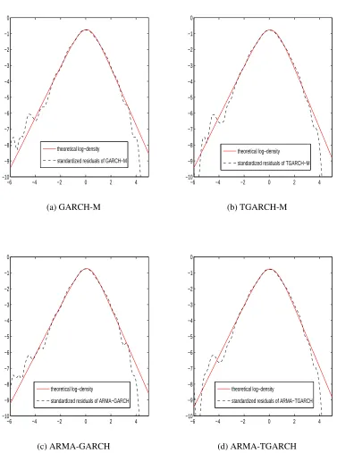
Figure 3.3 plots the log-densities of observed residuals vs. their theoretical distribution for different GARCH models. Similarly, there is a high degree of consistency of residuals’ dis-tribution between GARCH/TGARCH-M and ARMA-GARCH/TGARCH models. Compared with Figure 3.2, the log-density curves of standardized residuals estimated by z-GARCH mod-els show a great improvement in fitting their theoretical distribution, even though they do not completely capture the behavior of their theoretical density in the tails. Given that, we conclude that GARCH models driven byz-distributed innovations perform better in fitting financial data. Based on that, we expect z-GARCH models have a much better performance in option pricing. The details will be discussed in Chapter 5.
Alternatively, we could use appropriate QQ plots to compare the standardized residuals to the normal or z distributions. However, we would then need to construct a QQ plot for the
18 Chapter3. Estimation of theGARCH Models
Table 3.2: GARCH and TGARCH parameters estimated by MLE with normal innovations using daily closing prices of S&P 500 from January 02,1988 to January 06, 2004
Parameters GARCH-M TGARCH-M ARMA-GARCH ARMA-TGARCH
c 1.1377×10⁻⁴ 1.1377×10⁻⁴ 9.87×10⁻⁴ 3.40×10⁻⁴
- - (2.63×10⁻⁴) (1.36×10⁻⁴)
ϕ1 - - -0.924 0.0131
- - (0.117) (8.8×10⁻³)
θ1 - - 0.916 7.21×10⁻³
- - (0.122) (8.8×10⁻³)
λ 0.0609 0.0441 -
-(0.0013) (0.0188) -
-α0 4.87×10⁻⁷ 1.096×10⁻⁶ 4.52×10⁻⁷ 9.53×10⁻⁷
(1.5×10⁻⁷) (2.6×10⁻⁷) (8.8×10⁻⁸) (1.21×10⁻⁷) α1 0.0413 0.0059 0.0402 5.15×10⁻³
(0.0058) 0.0043 (2.99×10⁻³) (5.23×10⁻³)
β1 0.954 0.9424 0.956 0.9461
(0.0065) 0.0143 (3.3×10⁻³) (4.4×10⁻³)
γ - 0.0783 - 0.0768
- (0.015) - (7.6×10⁻³)
σ0 0.0072 0.0061 0.0072 0.0062
LLF 1.3160×10⁴ 1.3192×10⁴ 1.3160×10⁴ 1.3192×10⁴
AIC −2.6312×10⁴ −2.6373×10⁴ −2.6308×10⁴ −2.6370×10⁴
3.3. ModelFittingAnalysis 19
Table 3.3: GARCH and TGARCH parameters estimated by MLE, which under the assumption onz-distributed noise, using daily closing prices of S&P 500 from January 02, 1988 to January 06, 2004
Note: in this table, the subscript inαzorβzdenote the z-distribution case.
Parameters GARCH-M TGARCH-M ARMA-GARCH ARMA-TGARCH
c 1.1377×10⁻⁴ 1.1377×10⁻⁴ 9.34×10⁻⁵ 6.973×10⁻⁴
- - (3.3×10⁻⁵) (2.42×10⁻⁴)
ϕ1 - - 0.8071 -0.9337
- - (0.0568) (0.0292)
θ1 - - -0.8494 0.9259
- - (0.0512) (0.0319)
λ 0.0565 0.0419 -
-(0.0158) (0.016) -
-α0 3.04×10⁻⁷ 7.83×10⁻⁶ 2.63×10⁻⁷ 6.30×10⁻⁷
(1.3×10⁻⁷) (2×10⁻⁷) (1.2×10⁻⁷) (1.88×10⁻⁷)
α1 0.0405 0.0075 0.0389 0.0072
(0.0065) (0.006) (0.0064) (0.0056)
β1 0.9568 0.9443 0.9589 0.9488
(0.0069) (0.009) (0.0066) (0.008)
γ - 0.0787 - 0.0745
- (0.015) - (0.0138)
αz 0.698 0.7654 0.6181 0.7625
(0.096) (0.112) (0.0977) (0.111)
βz 0.7901 0.901 0.7273 0.9053
(0.119) (0.147) (0.126) (0.147)
σ0 0.0071 0.0059 0.0071 0.0059
LLF 1.3299×10⁴ 1.3322×10⁴ 1.3306×10⁴ 1.3323×10⁴
AIC −2.6585×10⁴ −2.6630×10⁴ −2.6596×10⁴ −2.6545×10⁴
20 Chapter3. Estimation of theGARCH Models
−6 −4 −2 0 2 4
−16 −14 −12 −10 −8 −6 −4 −2 0
theoretical log−density N(0,1) standardized residuals of GARCH−M standardized residuals of ARMA−GARCH
(a) GARCH models
−6 −4 −2 0 2 4
−16 −14 −12 −10 −8 −6 −4 −2 0
theoretical log−density N(0,1)
standardized residuals of TGARCH−M standardized residuals of ARMA−TGARCH
(b) TGARCH models
3.3. ModelFittingAnalysis 21
−6 −4 −2 0 2 4
−10 −9 −8 −7 −6 −5 −4 −3 −2 −1 0 theoretical log−density standardized residuals of GARCH−M
(a) GARCH-M
−6 −4 −2 0 2 4
−10 −9 −8 −7 −6 −5 −4 −3 −2 −1 0 theoretical log−density standardized residuals of TGARCH−M
(b) TGARCH-M
−6 −4 −2 0 2 4
−10 −9 −8 −7 −6 −5 −4 −3 −2 −1 0 theoretical log−density
standardized residuals of ARMA−GARCH
(c) ARMA-GARCH
−6 −4 −2 0 2 4
−10 −9 −8 −7 −6 −5 −4 −3 −2 −1 0 theoretical log−density
standardized residuals of ARMA−TGARCH
(d) ARMA-TGARCH
Chapter 4
Risk Neutral Measures Under GARCH
Models
All the definitions given in this Chapter are taken from Badescu [Bad07] who gives the ap-propriate references and attribution. These are given here in order to make this thesis self contained. When a definition or theorem does not have an explicit reference, it can be found in Badescu.
In this Chapter, we introduce two candidates of risk neutral measures which one can utilize for option pricing and normal and non-normal applications for discrete time GARCH models. In Section 4.1 we introduce certain notation, definitions and preliminary results which are very useful in constructing martingale measures. In Section 4.2 we describe two well known risk measures defined for discrete time markets, conditional Esscher transform and the extended Girsanov principle. The application of these two risk neutral measure for GARCH models to derive their risk neutralized dynamics will be introduced in Section 4.3.
4.1
Definitions and Notations
In discrete time financial models, trading dates are considered to form a discrete time index
{t|t=0,1, ...,T}whereT <∞is the finite expiration time. The time indextrefers to trading day andT is the expiration time in trading days. Corresponding to this time scale, the interest rate
ris daily interest rate. Denote (Ω,F,Ft,P) as a complete filtered probability space, wherePis
the historical probability measure andFt is a sequence of increasingσ-fields ofF containing
all information up to time t. We can assumeF0 = {0,Ω}andFT =F.
In order to price options written on a single stock, the financial market can be simplified as one consisting of only a reference asset or bondS0
t and a risky securitySt adapted to the
filtrationF. The dynamics of the bondS0t isS0t =e−∑tk=1rk, wherert is aFt-predictable process
is the interest rate over the period [t−1,t]. The discounted stock price is thus ˜St = e−
∑t
k=1rkS
t.
In our numerical experiments, we consider a constant continuously compounded risk-free rate
rfor the whole period so thatS0t =e−rtand ˜St =e−rtSt.
An arbitrage strategy aims at exploiting price differentials that exist as a result of market inefficiencies. To avoid arbitrage opportunities, we assume that the price process admits an equivalent martingale measure (EMM).
4.1. Definitions andNotations 23
Definition 4.1.1 (EMM [Bad07]) A probability measure Q is an equivalent martingale mea-sure w.r.t. to P if the following relations have been satisfied:
• Q≈ P (i.e. ∀B∈ F, Q(B)=0⇔ P(B)=0)
• the discounted price processS˜tis a martingale under Q w.r.t. toFt, that is EQ[ ˜St|Ft−1]=
˜
St−1
Let yt = lnSSt−t1 be the continuously compounded (log) return process, the above martingale
condition of discounted stock price can be replaced by :
EQ[eyt|F
t−1]= er.
Let Me(P) = {Q|Qis an EMM w.r.t. P}, where, Me(P) is the set of all martingale measures
equivalent toP.
Options are part of a larger class of financial derivatives. In our study we only focus on evaluating European options.
Example 4.1.2 European Options
• Call option
An option which conveys the right to buy an asset at the expiration time T for a fixed predefined strike price X is called a call.The payofffunction is :
hCall(ST)=
ST−X if ST > X
0 otherwise. (4.1)
• Put option
An option which conveys the right to sell an asset at the expiration time T for a fixed predefined strike price X is called a put. The payofffunction is :
hput(ST)=
X−ST if ST <X
0 otherwise.
We denoteΠCallt andΠPutt as the prices at timetof the Call and Put contracts.
24 Chapter4. RiskNeutralMeasuresUnderGARCH Models
Definition 4.1.3 (Badescu [Bad07]) Suppose that the set of all equivalent martingale mea-sures Me(P) is nonempty. Then the family of arbitrage-free prices at time t of a derivative security with payoffh(ST)is non-empty and is given by:
ΠQ
t (h(ST))=
{
EQ[e−r(T−t)h(ST)|Ft
]
|Q∈Me(P), EQ[h(ST)|Ft]<∞
}
In the next section we will discuss several most important risk-neutral measures used in the discrete time framework. Here, we state a lemma first, which will be utilized in constructing risk-neutral measures throughout this and subsequent chapter.
Lemma 4.1.4 (Badescu [Bad07]) Let P and Q be equivalent measures defined on on the mea-surable space(Ω,F). Then there exists an almost surely positive r.v. Ztsuch that EP[Zt|Gt]=1 and Q(A)= EP[I
AZt|Gt]for all A ∈ Gt (Gt is a finite sub-σ-algebra ofF). Here, ZT is called the Radon-Nikodym derivative on the filtrationGT. Then for any0 ≤ t ≤ T we have: P1: the conditional Radon-Nikodym derivative of Q w.r.t. P onGT is given by:
Zt := dQ
dPGt = E P[dQ
dPGt ]
.
P2: for anyGt(s≥t)and Q-integrable measurable function g,we have:
EQ[g|Gt]=
EP[Zsg|Gt] Zt
.
4.2
Risk Neutral Measures
During the recent decades, some of the widely used risk neutral measures are identified for general discrete time models. The stochastic discount factor (SDF) approach which is a com-mon approach, whose relation with the risk neutral valuation relationship (RNVR) principle is justified by an equilibrium argument. The minimal martingale measure (MMM) constructed by Follmer and Schweizer [FS91] was also studied in the financial literature. Another two well known tools are the conditional Esscher transform, which was first applied to option pricing by Gerber and Shiu [GS94], and the extended Girsanov principle (EGP) introduced by Elliot and Madan [EM98]. Badescu [Bad07] investigated some relationships between the Esscher transform, SDF and MMM and utility maximization. He proposed that the Esscher transform and EGP are two good candidate risk neutral measures, and the Esscher transform performs best for option pricing. Hence, we restrict our attention to these two measures in our thesis.
4.2.1
Conditional Esscher Transform
4.2. RiskNeutralMeasures 25
time series models. A conditional version of the Esscher transform was proposed by Buhlmann
et al. [BDES96] for a more general discrete model. The conditional version is related to a utility maximization problem for some specific form of the utility function.
Suppose that the conditional moment generating function of the returnsyt w.r.t. Ft−1exists
for allt, 0≤t ≤T:
MyP
t|Ft−1(c)=E
p[ecyt|F
t−1]<∞, c∈D⊆R.
Definition 4.2.1 (Conditional Esscher transform [GS94]) Denote δt as a predictable pro-cess w.r.t. aσ-algebra Gt. The probability measureP is called the conditional Esscher trans-ˆ formed measure of P if conditional moment generating functions exist:
dPˆ dPGt
=
t
∏
k=1
eδkXk
MXk|Gk−1(δk)
, (4.2)
where, Xt represents the stochastic process and δt is denoted as the Esscher parameter with respect to the filtrationGt.
Based on the Gerber and Shiu [GS94] formulation, we can characterize the Esscher risk-neutralized measure by the following theorem.
Theorem 4.2.2 (Badescu [Bad07]) Let the process Zt defined by:
Zt = t
∏
k=1
eδ∗kyk
MP yk|Fk−1(δ
∗
k)
,
where Z0= 1andδ∗k is a predictable process andδ∗k is the unique solution of the equation:
MyP
k|Fk−1(1+δk)=e
rMP
yk|Fk−1(δk), (4.3)
for all k∈1...T . Let the measure Qessbe defined by:
dQess
dP = ZT,
ThenQessis called the conditional Esscher transform of Pgenerated by the process y
t and the
Esscher parameterδt.
The conditional Esscher transform price of a contingent claim with payofffunctionh(ST)
is
ΠQess
t
( h(ST)
)
= EQess[e−r(T−t)h(ST)|Gt
]
.
26 Chapter4. RiskNeutralMeasuresUnderGARCH Models
4.2.2
Extended Girsanov Principle
The extended Girsanov Principle was introduced by Elliot and Madan [EM98] and gives an-other tool in choosing a probability measures within the infinite class of equivalent martingale measures under the discrete time framework.
The construction of the EGP transform is similar to the minimal martingale measure ap-proach, which depends on the multiplicative Doob decomposition of the discounted stock price.
e
St =Se0AtMt ,
whereMtis anGtmartingale andAtis a predictable process with respect toGt. The processAt
is given by the unique representation:
At = t
∏
k=1
EP[ eSk e Sk−1
|Gk−1
]
and where Mtis defined by:
Mt =
e St
e S0At
. (4.4)
According to Eq. (4.4), we can easily show thatMt is aP-martingale:
EP[Mt|Gt−1
]
= EP[ eSt e St−1At
Gt−1
]
= eSt−1E
P[ eSk
e
Sk−1|Gk−1
]
˜
S0At−1
= Mt−1.
The dynamics of the discounted stock price process underPhas the following representation
e
St =Set−1eνtWt . (4.5)
whereWt = Mt/Mt−1 is aGt martingale underPwith the unit mean and νt represents the one
period discounted excess returns meeting the following relation:
νt =−r+lnEP[eyt|Gt−1].
Definition 4.2.3 (Extended Girsanov Principle [Bad07]) A probability Q with respect toG is said to satisfy the Extended Girsanov Principle (EGP) if the conditional law of the discounted stock price under the new measure is equal to the conditional law where their martingale component from the multiplicative Doob decomposition prior to the change of measure:
LQ
eSt
e St−1
Gt−1
= LP(W
t|Gt−1) (4.6)
Thus, the discounted stock price eSt is a martingale under Q. The form of the