Performance Analysis of a Non Linear Process
Using Different PID Control Techniques
K. Sujitha1, R. Kalaiyarasi2, J. Nancy Amala Geetha3, P. Aravind4
UG Student, Department of ICE, Saranathan College of Engineering, Trichy, Tamil Nadu, India1,2,3
Assistant Professor, Department of ICE, Saranathan College of Engineering, Trichy, Tamil Nadu, India4
ABSTRACT: Industries are the huge developing areas in which all the complex systems are involved. They involve
controlling and tuning of the controllers of processes with streams like gases, liquids, powders, slurries etc.[2] They exhibit variations due to the changes in the operating level. This, in fact is the very nature of a non linear process. So, for this reason, researcher prefers controller design and tuning by specifying their design level of operation. This performance changes may be tolerable in some applications and unacceptable in others. In this paper, non linear process of a spherical tank is controlled and tuned using certain methods such as damped oscillation method, modified ZN method,[1] TL, ZNCL methods[2][6]. Here the controllers are designed stimulated using mat lab simulink. The best among PID controller settings is identified by time domain analysis.
KEY WORDS: PID Controller, Ziegler-Nichols Tuning Method, Set point Tracking, Non-Linear Process
I.INTRODUCTION
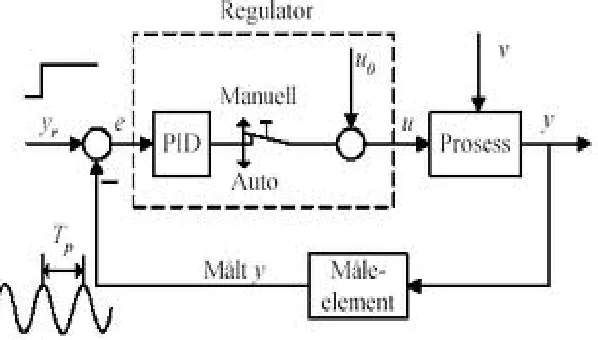
In the earlier days, industries worked with PID controllers. These controllers are commercially available and these are mostly used in process control industries till now. Later on, various methods of tuning have been discovered.[4] These methods resulted in better performance and acceptance in the industries. Even though they are widely used, in gas plant and storage of cryogenic liquids.PID controller is a widely used to control most of industries like automation and industrial processes because of its good efficiency and simplicity for the non linear process and they stand only for their certain specifications like rise time, overshoot etc..These type of controllers uses algorithms for tuning purpose. Further in two methods such as open and closed loop methods the controllers are tuned.[5] In open loop, we have to tune the controller in manual mode but in case of closed loop the controllers are tuned in automatic mode. In the spherical tank is divided into two operating region. Each of the region based as First order process with Dead Time(FOPDT).[3]Thus the response of four different type of controllers is obtained using MATLAB simulink and the response gives better set point tracking.
II.CONTROLLER DESIGN
The Different Types of Tuning Methods used for the Non Linear processes are[6] 1.Ziegler-Nichols method
2.Modified ZN method 3.Tyreus-Luyben method 4.Damped Oscillation method
5.Minimum Error Criteria(IAE,ISE,ITAE)
A.Closed Loop ZN Method(Ultimate Cycle)
It is based on adjusting a closed loop until steady oscillations occur. This is based on frequency response analysis.(from the bode plot and root locus technique we can calculate these parameters)[1].
Ultimate Gain= ku=1/m
period of Cycling = pu =2π/ωc0min/cycle
Table1: Controller Parameters for Closed Loop Ziegler-Nichols Method
Controller KP KI KD
P 0.5kcu - -
PI 0.45kcu Pu/1.2 -
PID 0.6kcu Pu/2 Pu/8
B.Tyreus-Luyben Method
It is equivalent to ZN method, the only difference is controller settings. It is applicable only for PI&PID controllers.[2] It has an advantage that consumption of time is reduced and the system is forced to margin in case of instability.
Table2: Controller Parameters for Closed Loop Tyreus-luyben Method)
Controller KP KI KD
PI Kcu/3.2 2.2Pu -
PID Kcu/3.2 2.2Pu Pu/6.3
C.Modified ZN Method
It is applicable in case of ¼ decay ratio and large overshoots attained these can be the resultant of variation in the set point. [2]This condition is unacceptable and hence we go for conventional methods like MZN.
Table3: Controller Parameters for Closed Loop Modified Ziegler-Nichols Method)
Controller KP KI KD
Some overshoot 0.33kcu Pu/2 Pu/3
No overshoot 0.2Kcu Pu/2 Pu/3
D. Damped Oscillation Method
In many plants, sustained oscillations for testing purposes are not allowable. So this method is more accurate than ultimate method.[2]By using only proportional action and starting with a low gain, the gain is adjusted until the transient response of the closed loop shows a decay ratio of ¼.the rest time and derivative time are based on the period of oscillation, P, which is always greater than the ultimate period Pu.
For PID control, TD=P/6 and TI=P/1.5
Table4: Controller Parameters for Closed Loop Damped Oscillation Method) Controller KP KI KD
P 1.1Gd - -
PI 1.1Gd Pd/2.6 -
The reason we choose these methods is that they give effective output performance than the other methods like IMC etc..which has been implemented by others.
III.MATHEMATICAL MODELLING
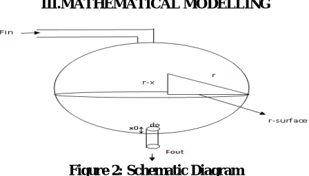
Figure 2: Schematic Diagram
The picture shown above is the spherical tank which has its own non linear dynamic behaviour. The spherical tank system consists of a maximum height of 0.6meter and its maximum radius is about 0.6 meter. The tank level at any instant can be measured by the combination of orifice and Differential pressure transmitter which has its output as (4 -20)mA. This obtained output is compared with the desired set point value of level .[5] The resultant error signal is amplified based on the controller specifications. The output of the controller is used to vary the flow rate of the inlet q1(t) of the spherical tank so that we can able to maintain the set point at our desired level of the tank. An Electro pneumatic converter can be used to convert the controller output of (4 -20)mA in to a pneumatic signal of (3-15) psi.So that the final control element will be able to throttle the inflow rate. [6]
Let us consider,
q1(t) -flow rate of input to the tank in m3/sec q2(t) -flow rate of output of the tank in m3/sec H - spherical tank Height in meter.
R – tank radius in meter (0.5 meter).
X0 - Thickness of the pipe in meter(0.04 meter).
By the law of conservation of mass ,the non-linear equation obtained for the spherical tank is, Q1(t)-Q2((t)=Ah1*dh1/dt
Where A=π*r2Radius on the surface of the fluid depends on the level (height) of fluid in the tank r=√2rh1-h12
therefore
A=π(2rhx-hx2) then
Q2(t)=√2g(h-x0),a=π(x0/2)2
Q(s)=a√2gH (s)/2(√h0-x0) = π(2rhx-hx)2SH(S)
By linearizing the non linearity in spherical tank, we get
H(S)/Q(S)=1/π(2rhx-hx2)S + a√2g/2(√hx-x0)
By applying the steady state condition, the linearized transfer function of the plant obtained is,
Y ( S ) = 0.036 e-2s
For step change at 60LPH U ( S ) 2.5s+1
For step change at 120LPH Y(S) = 0.057 e-2s
IV.ANALYSIS
Thus we have tunned the controllers by this four methods and we examine the results as shown in the table:
A.Performance Criteria for region 1 :
Table 5: Time Domain Analysis for First Region at 60LPH:
Methods Rise time(tr)
in seconds
Settling time(ts) in
seconds
Peak(tp) Peak
overshoot(Mp)
% Modern
Zeigler-Nichols
4.6 12.1 1.89 7.7
Zeigler-Nichols 1.03 6.28 1.24 24
Tyreus-Luyben 26.5 48.8 0.996 0
Damped Oscillation 0.154 10.4 3.47 171
Table 6: Error Analysis for First Region at 60LPH
Methods IAE ITAE ISE
Modified ZN 7.126 6.476 2.0767
Zeigler-Nichols 3.7014 4.4455 980.195
Tyreus-Luyben 3.695 395.54 2.838
Damped Oscillation 2.7357 7.5060 2.8225
Here we can recognize that the peak overshoot and the corresponding settling time is less in MZN when compared to other methods. It gives better settling time and overshoot.
B. Time domain Performance Criteria :
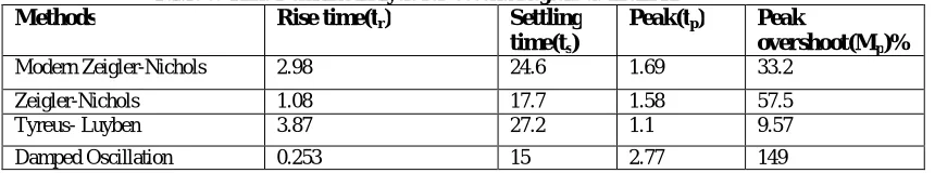
Table 7: Time Domain Analysis for Second Region at 120LPH:
Methods Rise time(tr) Settling
time(ts)
Peak(tp) Peak
overshoot(Mp)%
Modern Zeigler-Nichols 2.98 24.6 1.69 33.2
Zeigler-Nichols 1.08 17.7 1.58 57.5
Tyreus- Luyben 3.87 27.2 1.1 9.57
Damped Oscillation 0.253 15 2.77 149
Table 8: Error Analysis for Second Region at 120LPH
METHODS IAE ITAE ISE
Modified ZN 7.165 3.451 4.390
Zeigler-nichols 4.258 2.381 2.104
Tyreus-luyben 3.712 1.544 8.745
Damped oscillation 2.716 3.969 5.921
Figure 3: Performance of Spherical Tank at 60LPH
Figure 4: Performance of Spherical Tank at 120LPH
V. CONCLUSION
Thus we select damped oscillations method is the best to control and tune the controller at minimum peak overshoot and settling time. But this is not the efficient result which may be further reduced with other methods like Modern Predictive Control etc. which we would try in our next paper. “BEST PERFORMANCE” is something we judge ourselves based on the goals of production, capabilities of the process, impact on down stream units and the desires of management. Nonlinear behaviour should not catch us by surprise. It is something we can know about our process in advance.
REFERENCES
1. Mohammad shahrokhi and alireza Zomorrode,”comparison of PID controller Tuning methods”,Department of chemical&petroleum Engineering,Sharif University of Technology.
2. Ziegler J.B Nichols N.B” optimum settings for automatic controllers” ASME transactions(1942). 3. Smith,C.A, A.B. copripio; “principles and practice of Automatic process control”.John wiley&sons,1984. 4. Luyben W.L,M.L.Luyben;”Essentials of process control”,McGraw-Hill,1997.
5. Krishnaswamy P.R.,B.E Mary Chan,and G.P. Rangaish;”Closed-Loop Tuning of control systems”. Chemicl engg., science(1987). 6. Process Control ( Principles and Applications) By Surekha Bhanot
-60 -40 -20 0 20 40
0 20 40 60 80 100 120
ZN-CL
TL
DOSC
MZN-20%OVERSHOO T
-100 -50 0 50 100
0 20 40 60 80 100 120
ZN-CL
TL
DOSC