On fractional correlation immunity of majority
functions
∗Chuan-Kun Wu
State Key Laboratory of Information Security, Institute of Software Chinese Academy of Sciences, Beijing 100190, China
Email: [email protected]
February 10, 2009
Abstract:
The correlation immunity is known as an important cryptographic measure of a Boolean function with respect to its resist against the correlation attack. This paper generalizes the concept of correlation immunity to be of a fractional value, called fractional correlation immunity, which is a fraction between 0 and 1, and correlation immune function is the extreme case when the fractional correlation immunity is 1. However when a function is not correlation immune in the tra-ditional sense, it may also has a nonzero fractional correlation immunity, which also indicates the resistance of the function against correlation attack.
This paper first shows how this generalized concept of fractional correlation im-munity is a reasonable measure on the resistance against the correlation attack, then studies the fractional correlation immunity of a special class of Boolean functions, i.e. majority functions, of which the subset of symmetric ones have been proved to have highest algebraic immunity. This paper shows that all the majority functions, including the symmetric ones and the non-symmetric ones, are not correlation immune. However their fractional correlation immunity ap-proaches to 1 when the number of variable grows. This means that this class of functions also have good resistance against correlation attack, although they are not correlation immune in the traditional sense.
Key words: Cryptography, Majority function, Correlation immunity, Walsh transform.
1
Introduction
The development of cryptographic algorithms have experienced different attacks. As a result of the attacks, different measurement about the resistance against the corresponding attacks are proposed. When correlation attack [7] was treated as a threat, the concept of
correlation immunity is proposed [6] as a measurement about the resistance that a nonlinear combination function has against the correlation attack. Recently a new attack known as the algebraic attack is proved to be very effective to many stream ciphers as well as to some block ciphers. As a measurement of the resistance of a nonlinear function against the algebraic attack, another measurement known as algebraic immunity is proposed. The idea of algebraic attack is to find an annihilator of the targeting combining function. By doing so, the process of algebraic attack is to solve a system of nonlinear equations. When the algebraic degree of the annihilator is low, the computational complexity to solve such a system of nonlinear equations is also low. So the effectiveness of algebraic attack depends on whether one can find such an annihilator with low algebraic degree. On the other hand, when the combining function is of high algebraic immunity, the algebraic degree of any of its annihilators cannot be very low. Hence, a significant job for the designers is to find combining functions with highest possible algebraic immunity. It has been proved [5] that the order of the algebraic immunity of a Boolean function innvariables cannot exceeddn2e. If a Boolean function has algebraic immunity of orderdn2e, then this function is said to have the highest algebraic immunity.
In 2004, Dalai [3] studied the majority functions to be a class of Boolean functions with highest algebraic immunity, and [4] further proves that the majority functions are the only symmetric Boolean functions in odd number of variables with maximum algebraic immu-nity. While algebraic immunity is an important cryptographic measurement, very often the best performance with one cryptographic measurement will sacrifice the performance with other cryptographic measurements. In this paper we study the correlation immunity of the generalized majority functions, which include the majority functions in odd number of variables and newly defined such functions in even number of variables.
2
The correlation immunity for nonlinear combining
func-tions
The concept of correlation immunity was proposed by Siegenthaler in 1984 [6]. It is a security measure against the correlation attack (also known as divide-and-conquer attack) of nonlinear combiners [7]. Therefore we first briefly describe the correlation attack of nonlinear combiners, which gives the rationale of why correlation immunity is a reasonable security measure against the correlation attack. This helps us to introduce the concept of fractional correlation immunity in the next section.
2.1 Preliminaries about Boolean functions
LetGF(2) be a finite field of two elements 0 and 1, andGFn(2) be ann-dimensional vector space over GF(2). A mapping fromGFn(2) into GF(2) is called a Boolean function inn
variables, denoted by f(x), where x = (x1, x2, ..., xn) is the shorthand form of a vector in
of this vector, and is denoted as WH(x). If WH(x) = n2, i.e., there are equal number of 0’s
and 1’s in the coordinates of x, thenx is called balanced.
For a Boolean functionf(x) in nvariables, whenx goes through all the possible values (vectors) of GFn(2), then f(x) will have 2n corresponding outputs. The vector of all the outputs off(x) is called thetruth tableoff(x), which has dimension 2n. Of coursex has to follow a particular order when going through all the possible values of GFn(2). If we treat a binary vector as the binary representation of an integer, then when the integer takes all the values from 0 to 2n−1, then the corresponding vector goes through all the elements in GFn(2). Traditionally, we let the value of the binary representation of the integer to
go from 0 incrementally to 2n−1. If we collect all the vectors where f(x) takes value 1,
then the collection is called the support of f(x), denoted as supp(f) = {x : f(x) = 1}. The number of 1’s in the truth table of f(x) is called the Hamming weight of f(x) and is denoted as WH(f). It is easy to see thatWH(f) is the number of elements in supp(f).
2.2 The correlation attack of nonlinear combiners
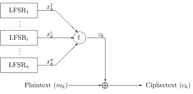
Nonlinear combiner is a popular pseudo-random sequence generator for stream ciphers. The basic structure of nonlinear combiner in stream ciphers is as shown in figure 1.
LFSRn
.. . LFSRi
.. . LFSR1
-@
@ @@R
f
?
L
-Plaintext (mk) - Ciphertext (ck)
xnk
xik zk
x1k
Figure 1: A nonlinear combiner of stream ciphers
The correlation attack proposed by Siegenthaler [7] makes use of the correlation informa-tion between the output sequence (zk) of the nonlinear combiner and each input sequence
(xik) of the combining functionf(x), and to use the statistical analysis trying to recover the initial state as well as the feedback function of each LFSRi individually. This approach is
also called divide and conquer attack, which significantly reduces the complexity than the brute force attack.
In the security analysis, it is always assumed that the structure of the generator is known, i.e. the lengths of each LFSR and the nonlinear combining function f(x). The attack proposed in [7] does not assume the knowledge of the primitive feedback polynomial of each LFSR which is only of certain limited amount to search for.
generators, i.e. each LFSRi of order ri generates an m-sequence of period pi = 2ri −1,
and there are Ri primitive polynomials of degree ri (which is the number of different m
-sequences of order ri such that they are not equivalent by cyclic shift). Then under the
brute force attack, the number of all the possible keys for the nonlinear combiner (different initial states and different feedback function of each of the LFSR have been taken into account) is
K =
n Y
i=1
Ri(2ri−1).
With the correlation attack, information about each input sequence (xi
k) can be extracted
from the output sequence (zk), and hence the attack can concentrate each of the individual
LFSR sequences, and the number of trials in the worst case is reduced to approximately
K0 =
n X
i=1
Ri2ri.
The correlation attack is a probabilistic attack which assumes some statistical properties of the combining function f(x). Assume in the ideal case that each of the LFSR’s in figure 1 produces a pseudo-random sequence with uniform probability distribution, i.e.
P rob(xik= 0) =P rob(xik= 1), and assume that P rob(zk= 0) =P rob(zk = 1). Let
P rob(zk=xik) =qi, (1)
and assume the plaintext comes from a memoryless binary source, which satisfies
P rob(yk= 0) =p0 (2)
Then it is easy to compute
P rob(ck⊕xjk= 0) = P rob(zk=xjk)·P rob(yk= 0)
+P rob(zk6=xjk)·P rob(yk= 1)
= 1−(p0+qj) + 2p0qj
= pe (3)
When j = 0, let x0
k be an hypothetical random variable which are independent of any xik (i > 0) and with uniform probability distribution. Then compute the correlation of sequences ck and xjk as
α=
N X
k=1
(1−2(ck⊕xjk)) =N −2
N X
k=1
(ck⊕xjk), j∈ {0,1, ..., n} (4)
By the central limit theorem, whenN is sufficiently large,α approaches to a normal distri-bution (or Gaussian distridistri-bution). In an attack, attackers use hypothetical LFSR of length
ri which produce sequence (x0k) for the testing. By choosing a nonzero initial state and
an arbitrary primitive polynomial as the feedback polynomial, compute the correlation α0
H1: There are N > ri coincidences between the output of the hypothetical LFSR and
LFSRi, referring to the above cases, this is the case whenα0 is the correlation between
zk and xik,i∈ {1,2, ..., n}.
H0: There are N > ri disagreement between the output of the hypothetical LFSR and
LFSRi, referring to the above cases, this is the case whenα0 is the correlation between
zk and x0k.
In order to make a decision about the two hypotheses, a threshold value T is needed. When α0 < T, then accept the hypothesis H0, and when α0 ≥ T, accept H1. Let the
probability density function of the probabilistic variableαbePα|Hk(x). Ifqi= 12 orp0 = 12,
then by Eqn. (3), we havepe= 12, in this case no decision can be made, because in this case
the probability distribution of α under the two hypotheses is the same. Here the discussed attack depends on the number of wrong decisions, i.e. the number of cases when α ≥ T. So we define a false alarm probability Pf = P rob(α ≥ T|H0). In order to determine an
appropriate threshold T, we also need to consider the probability Pm =P rob(α < T|H1).
We have
Pf =
Z ∞
T
Pα|H0(x)dx (5)
Pm = Z T
−∞Pα|H1(x)dx (6)
With the help of the function
Q(x) = √1
2π Z ∞
x e
−y22dy (7)
we can get the following expressions:
Pf = Q(| T
√
N|) (8)
Pm = Q(|
N(2pe−1)−T
2√Np
pe(1−pe)|
) (9)
Denote by
γ0= N(2pe−1)−T
2√Np
pe(1−pe)
, (10)
then the expression of Pf and Pm can be written as
Pf = Q(|
√
N(2pe−1)−2γ0
q
pe(1−pe)|), (11)
Pm = Q(|γ0|). (12)
In order to attack the stream cipher model as in figure 1, the following process is to be taken: first to determine the probability qi by f(x), and to determine the probability p0
according to the coding method of the plaintext, then computepe using Eqn. (3). For any
chosen probability Pm, by Eqn. (12) it is known that γ0 is a constant, and from Eqn. (11)
recover LFSRi, choose an arbitrary primitive polynomial as its feedback polynomial and an
arbitrary nonzero state as its initial state, and let it produce a sequence, then compute the correlation between this sequence and the ciphertext sequence. For any event with α≥T,
H0is accepted, i.e., the LSFRi is supposed to have been recovered. However the probability
of event α≥T isPf, and our decision may be wrong. So we need to test more ciphertexts
for all the eventsα≥T. If for all the 2ri−1 different states, the decision is always to reject
H1, then change another primitive polynomial and to repeat the test. In the worst case we
need to test for about Ri2ri times. The false alarm probability depends on the length of
ciphertext N. Choose N1 such that
Pf =
1
Ri2ri (13)
then by Eqn. (11) we have
1
Ri2ri
=Q(|p
N1(2pe−1)−2γ0
q
pe(1−pe)|) (14)
using the inequality
Q(x)< 1
22
−x2
2 , x >0 (15)
we can get an upper bound ofN1:
N1 <
1
√
2
p
ln(Ri2ri−1) +γ0
p
pe(1−pe)
pe−12
2
. (16)
The above is a brief description of the correlation attack which is mainly from [7]. The inclusion of the description is to help to understand how correlation immunity and conse-quently the fractional correlation immunity serves as a counter-measure against the corre-lation attack.
The upper bound in (16) gives the length of required ciphertext to enable the attack on the model in figure 1. If the length of the ciphertext is no less than this upper bound, then when performing such an attack, the number of tests can be minimized and when a decision is made, the probability of false alarm is minimized. More detailed description of the correlation attack can be found in [7].
In order to resist the correlation attack as described above, the combining functionf(x) needs to have some special properties. Siegenthaler [6] introduced the concept of correla-tion immunity of Boolean funccorrela-tions, and we will see how such funccorrela-tions can have resistance against the correlation attack. Then we will show how much resistance a fractionally cor-relation immune function would have against the corcor-relation attack.
2.3 Correlation immunity as a counter-measure against the correlation attack
Definition 1 Let f(x) be a Boolean function in n variables. Treat (x1, x2, ..., xn) as n
random variables overGF(2)that are independent and have uniform probability distribution, i.e. each xi is equally likely to be 0 or 1. If for any 1 ≤i1 < i2 <· · ·< ik ≤n, the value
of f(x)is statistically independent of (xi1, xi2, ..., xik), i.e., for any (a1, a2, ..., ak)∈GF
k(2)
and any c ∈ GF(2), we always have P rob(f(x) = c|(xi1, xi2, ..., xik) = (a1, a2, ..., ak)) =
P rob(f(x) = c), then f(x) is said to be correlation immune of order k, or briefly k -order correlation immune. The maximum number of ksuch thatf(x)isk-order correlation immune is called the correlation immunity of f(x), and is denoted as CI(f) =k.
There are many different but equivalent definitions of correlation immunity. One of such alternatives is that, when a Boolean function f(x) is correlation immune of order k, then its support supp(f) has the property that, the vector formed from any (i1, i2,· · ·, ik)
coordinates ofsupp(f) will equally likely to be any vectors inGFk(2) whenxgoes through
all the values in supp(f). In particular, when k = 1, then the support of a correlation immune function has the property that, any coordinate of the vectors insupp(f) has equal chances to be 0 or 1. It is trivial to verify that, if a Boolean function is correlation immune of order k, then for anym < k, this function is also correlation immune of orderm.
Consider a simple case, assume that the combining function in the nonlinear combiner is correlation of order 1, i.e., for anyxi, the probability thatf(x) takes any value is not affected
by a pre-fixed value of xi. By Eqn. (3) we have thatpe = 12. Taking it into Eqn. (16), we
get an infinity upper bound of N1, which means that the number of ciphertext to conduct
such an attack may be infinity and hence not possible.
While a Boolean function of correlation immunity of order 1 being the combining function seems to resist the correlation attack, it is only to the case when consider the individual LFSR’s. When a linear combination of a few of the LFSR’s is considered, higher order correlation immunity is correspondingly required to resist the correlation attack.
3
The fractional correlation immunity as a counter-measure
against the correlation attack
It is noted that the correlation immunity is a cryptographic measure about the resistance against correlation attack, there can be cases where although a combining function is not correlation immune, however the correlation attack still consumes large amount of compu-tation due to the function being “almost” correlation immune. We hereby define a measure about how close a function is to being correlation immune. This only makes sense for the functions that are not correlation immune. Motivated by Eqn. (3) and Eqn. (4), let us first consider a simple case, i.e., the balancedness of the i-th coordinate of all the vectors in
supp(f). If it has a good balance, thenf(x) has small correlation withxi. If it is balanced,
the number of 0’s and that of 1’s in the i-th coordinates of vectorsx insupp(f), i.e.,
ε(i)(f) =| X
x∈supp(f)
(−1)xi|=|W
H(f)−2 X
x∈supp(f)
xi|.
By this definition, it is easy to see that the idea of correlation immunity is to find the maximum value of these relative correlations. If the maximum value is 0, then f(x) must be correlation immune (of order 1 or higher), otherwise f(x) is not correlation immune. However, in the case f(x) is not correlation immune, the value of ε(i)(f) varies which indicates the different degrees that f(x) has correlation with xi. The correlation of f(x)
with any variable is hence defined as
ε(f) = max
i∈{1,2,...,n}ε
(i)(f).
For this consideration, we define the fractional correlation immunityof f(x) as
F CI(f) = 1− ε(f)
WH(f)
= 1− 1
WH(f)
max
i∈{1,2,...,n}|WH(f)−2 X
x∈supp(f)
xi| (17)
It is seen from Eqn. (17) that 0≤F CI(f)≤1. WhenF CI(f) = 1, it means that f(x) is correlation immune (of order 1). Another extreme case is whenF CI(f) = 0, this means that there exists i such that xi = 0 (or xi = 1) always holds for all x ∈ supp(f), which
means that the correlation between f(x) and thisxi is high (the highest possible case). In
general, the fractional correlation immunity F CI(f) is a fractional value between 0 and 1, instead of integral value as the traditional definition of correlation immunity.
Now we take a look at what the fractional correlation immunity has to do with the correlation attacks proposed by Siegenthaler. Let ibe such an index satisfying that
F CI(f) = 1− 1
WH(f)
(|WH(f)−2 X
x∈supp(f)
xi|)=∆ε.
Then we have
P rob(xi= 1|f(x) = 1) =
P x∈supp(f)
xi
|supp(f)| =
P x∈supp(f)
xi
WH(f)
and
P rob(xi = 0|f(x) = 0) =
|supp(f)| − P x∈supp(f)
xi
|supp(f)|
=
2n−WH(f)−( P x∈GFn(2)
xi− P x∈supp(f)
xi)
2n−W H(f)
=
2n−1−W
H(f) + P x∈supp(f)
xi
2n−W H(f)
.
Hence by Eqn. (1) we have
= P rob(f(x) = 1)P rob(xi = 1|f(x) = 1) +P rob(f(x) = 0)P rob(xi = 0|f(x) = 0)
= WH(f) 2n ·
P x∈supp(f)
xi
WH(f)
+ 2
n−WH(f)
2n ·
2n−1−W
H(f) + P x∈supp(f)
xi
2n−W H(f)
= 1
2n(2 n−1
−WH(f)−2 X
x∈supp(f)
xi)
= 1
2 −
WH(f)
2n (1−ε) (18)
Ifεis very close to 0, thenqiis very different from 12. Particularly whenf(x) is balanced
which is often practically required, then qi is very close to 1 or 0, in which case, we have high confidence to have either f(x) =xi or f(x) =xi⊕1. Consequently by Eqn. (3), we
get that pe ≈ p0 or pe ≈ 1−p0. It is assumed that p0 6= 12, otherwise we would always
have pe = 12 and hence the correlation attack does not work. It is also easy to verify that
these are cases when |pe− 12| reaches the maximum value, and by (16) we know that the
minimum amount of data is needed to perform a correlation attack.
Ifεis very close to 1, thenqi is very close to 12, and by Eqn. (3), pe is also very close to
1
2, and consequently large amount of ciphertext is required to perform a correlation attack.
Although such an attack is possible, however, when ε is so close to 1 that results in the bound of (16) to be too large to reach in practice, then the correlation attack becomes practically impossible.
To be more precise, taking Eqn. (18) into Eqn. (3) we have
pe= 1−(p0+qi)−2p0qi =
1 2+
WH(f)
2n (1−ε)(
1 2 −p0)
It is obvious that when ε is very close to 1, then pe is also very close to 12, and hence
Eqn. (16) gives a very large upper bound.
Perhaps an upper bound of the size of text needed to conduct an attack is less convincing, because the actual number of text needed can be much smaller than the upper bound. To be more convincing, here we introduce a lower bound given in [8].
It is easy to prove that for the functionQ(x) defined in Eqn. (7), we have
Q(x)> 1
4e
−x2
, x >0
Taking into Eqn. (14) we have
N1 >
p
ln(Ri2ri)−2 ln 2 + 2γ0ppe(1−pe)
2pe−1
!2
> ln(Ri2
ri)−2 ln 2
[WH(f)(12 −p0)(1−ε)]2
(19)
This means that as long as the fractional correlation immunity of f(x) is sufficiently close to 1, then pecan be sufficiently close to 12 and henceN1 is sufficiently large, too large to be
The concept of higher order fractional correlation immunity has similar motivation to that of higher order correlation immunity, i.e., it is to measure the probability of event (f(x) = xi1 ⊕xi2 ⊕ · · · ⊕xik) and a corresponding modified correlation attack, for any
possible 1≤i1 < i2 <· · ·< ik ≤n.
4
On the Walsh characterization of correlation immunity and
fractional correlation immunity
Walsh transform has been a very useful tool in analyzing cryptographic properties of Boolean functions. Here we use Walsh transform to study the correlation immunity of majority functions.
Definition 2 Letf(x)be a Boolean function innvariables. The following function defined on the field of real numbers
Sf(w) =
2n −1
X
x=0
f(x)(−1)w·x (20)
is called the Walsh transform of f(x), and the truthtable of Sf(w) is called the Walsh
spectrum of f(x), where w·x=w1x1⊕w2x2⊕ · · · ⊕wnxn is the inner product of vectors w and x. For any w∈GFn(2), the value of S
f(w) is called the Walsh spectrum off(x) on w.
In the implementation of electronic circuits, it would be more convenient to use{−1, 1} to represent the domain of binary functions than to use {0, 1}, and hence the following transform is used to map {0, 1} to {−1, 1}:
F(x) = (−1)f(x).
By this transform, the Boolean function f(x) is then mapped to function F(x) on the domain{−1, 1}. The Walsh transform can also apply toF(x) as:
SF(w) =
2n−1
X
x=0
F(x)(−1)w·x (21)
Note that when the Boolean function f(x) is also treated as a binary real valued-function, the Walsh transform remains the same. By this treatment, the two functions can be con-verted to each other:
F(x) = 1−2f(x)
Then, the Walsh transform of F(x) can be converted from the Walsh transform off(x), i.e.
SF(w) =
2n −1
X
x=0
(1−2f(x))(−1)w·x
=
2n −1
X
x=0
(−1)w·x−2
2n −1
X
x=0
f(x)(−1)w·x
=
(
2n−2Sf(w) ifw= 0
On the other hand, the Walsh transform off(x) can be converted from the Walsh transform of F(x):
Sf(w) = (
2n−1−12SF(w) ifw= 0
−12SF(w) ifw6= 0
Note that the Walsh transform on F(x) is also known as the type II Walsh transform of
f(x), and is denoted as
S(f)(w) = 2n
−1
X
x=0
(−1)f(x)+w·x.
And hence Sf(w) is called the type I Walsh transform of f(x). The following study will
mainly use type II Walsh transform, and without confusion, we will simply call it Walsh transform, and its type can be distinguished by the notation.
There is a very good Walsh spectrum description about the correlation immunity of Boolean functions.
Lemma 1 (Xiao-Massey[9]) A sufficient and necessary condition for f(x) ∈ Fn to be
correlation immune of order k is that for any w ∈GFn(2) with 1≤W
H(w) ≤k, we have S(f)(w) = 0.
Although we used the type II Walsh spectrum to describe the correlation immunity in the above lemma, it is obvious that to use any type of Walsh spectrum will be the same, because for any nonzero w, we always have thatSf(w) = 0 if and only if S(f)(w) = 0.
In order to compute the fractional correlation immunity of a Boolean function, motivated by lemma 1, we will seek a Walsh spectrum description. It is easy to deduce that the Walsh spectrum of f(x) on ei (where ei is such a vector in GFn(2) that its i-th coordinate is 1
and 0 elsewhere) is
S(f)(ei) =
X
x∈GFn(2)
(−1)f(x)+w·x
= −2 X
x∈supp(f)
(−1)ei·x
= −2 X
x∈supp(f)
(−1)xi
= −2 X
x∈supp(f)
(1−2xi)
= 4 X
x∈supp(f)
xi−2WH(f)
Therefore by Eqn. (17) we have
F CI(f) = 1− 1 2WH(f)
max
i |S(f)(ei)| (22)
The above defined fractional correlation immunity corresponds to the traditional corre-lation immunity of order 1, i.e., the correcorre-lation of the output of the function with only one of the inputs is considered. Similar to the correlation immunity of order higher than 1, it is easy to extend the concept of fractional correlation immunity to the case when consider the correlation of the output of the function with a linear combination of its input vari-ables. Note that the basic correlation attack considers qi = P rob(f(x) = xi), in general
case, we may consider a non-zero linear combination of the LFSR sequences, and the linear combination can be written as w.x, where w∈ GFn(2) is the coefficient vector. Now the
probability
qw =P rob(f(x) =w·x)
needs to be considered. Whenw=ei, we havew·x=xiwhich is the special case. However
even in the general case, one cannot afford to count all the possible linear combinations in a practical attack. So we can restrict that there are at most k LFSR sequences involved in a linear combination, where k is a security parameter. So we need to consider all the linear combinationsw·xwith 1≤WH(w)≤k. Similar to the analysis of how the fractional
correlation immunity is related to the basic correlation attack, we can define the k-order fractional correlation immunity of f(x) inn Variables as follows: First we define
ε(w)(f) =| X
x∈supp(f)
(−1)w·x|
to be the correlation between the output of f(x) and the linear combination of its inputs with was the coefficient vector of the linear combination, and define
εk(f) = max w: 1≤WH(w)≤k
ε(w)(f)
Then the k-order fractional correlation immunity of f(x) is defined as
F CIk(f) = 1− εk(f) WH(f)
In order to compute the fractional correlation immunity of a Boolean function, motivated by lemma 1, we will seek a Walsh spectrum description. It is easy to deduce that the Walsh spectrum of f(x) on ei (as defined before, ei is such a vector in GFn(2) that its i-th
coordinate is 1 and 0 elsewhere) is
Sf(ei) =
X
x∈GFn(2)
f(x)(−1)ei·x
= X
x∈supp(f)
(−1)ei·x
= X
x∈supp(f)
(−1)xi
= X
x∈supp(f)
(1−2xi)
= WH(f)−2 X
x∈supp(f)
Therefore we have
F CI(f) = 1− 1
WH(f)
max
i |Sf(ei)| (23)
Given the relationship of the two types of Walsh spectrums, we haveSf(ei) =−21S(f)(ei),
and hence the fractional correlation immunity can be represented as
F CI(f) = 1− 1 2WH(f)
max
i |S(f)(ei)| (24)
We will use the concept of fractional correlation immunity to study the majority functions in the next section, and will see that although the majority functions are not correlation immune in the traditional sense, but their fractional correlation immunity tends to approach to 1 with the increase ofn, which means that they also have a good resistance against the correlation attack.
For the case of k-order fractional correlation immunity, with similar analysis as above, it is easy to deduce the following:
F CIk(f) = 1−
max
w: 1≤WH(w)≤k
|Sf(w)|
WH(f)
. (25)
When k = 1, it becomes the factional correlation immunity as defined above, i.e., the specification of “1-order” is often omitted in the description.
Recall that if functionf(x) is correlation immune of orderk, then it must be correlation immune of any order m < k as well. In other words, if we write CIk(f) to be the k
-order correlation immunity of f(x), i.e., CIk(f) = 1 means that function f(x) is k-order
correlation immune (note that herekmay not be the largest correlation immunity off(x)), and CIk(f) = 0 means that f(x) is not k-order correlation immune. Then CIk(f) = 1
implies thatCIm(f) = 1 holds for anym < k. Alternatively we can write this as
CIk(f)≤CIm(f), m < k
where CIi(f) only takes integral value 0 or 1.
Note from Eqn. (25) that the introduction of fractional correlation immunity also holds a similar inequality
F CIk(f)≤F CIm(f), m < k (26)
which generalizes the above inequality on correlation immunity to the fractional case. This can be understood as: if f(x) is correlation immune of orderk (k can be 0), then it must be correlation of orderk−1. However perhaps it may not be correlation immune of order
5
Majority functions and their Walsh spectrum
characteri-zation
Symmetric Boolean functions have many interesting properties [2], and those in odd number of variables have maximum algebraic immunity [4]. A special subset of symmetric Boolean functions are the majority functions, who seem to be the only symmetric functions that reach the maximum algebraic immunity for small number of variables [1].
In this paper, we will extend the concept of majority functions by introducing set major-ity functions. The concept of set majormajor-ity function is not very new, but the term is never specifically named before. It should be noted that a large number of set majority functions in even number of variables are not symmtric. It is also noted that the study on majority functions so far has mainly been restricted to those symmetric ones, except [3] where the nonlinearity of balanced set majority functions in even number of variables are considered.
5.1 Definitions
Definition 3 Let n be an odd number. The following defined Boolean function f(x) in n
variables is called a majority function:
f(x) =
(
0, if WH(x)≤ n−21;
1, if WH(x)≥ n+12 .
(27)
The natural meaning of the above defined majority function is that, when the majority of then-bit input has value 1, then the function outputs 1 which means a TRUE value, and when the majority of the input has value 0, the function outputs 0 which means FALSE.
The definition of majority function is very natural for the case when the input has odd number of coordinates, i.e. the number of inputsnof the function is an odd number. When
nis even, there is no natural way of defining majority functions, as there are cases where the input has equal number of 0 values and 1 values. For this case, we generalize the concept of majority function as follows:
Definition 4 Let n be an even number. Define S = {x ∈ GFn(2) : WH(x) = n2} and
A⊆S. Then
fA(x) = (
0, if WH(x)< n2 or x∈A;
1, if WH(x)> n2 or x∈(S\A).
(28)
is called a set majority function.
There are two extreme cases of the set majority functions, that is whenA=S and when
A=φ which is an empty set. WhenA=S, Eqn. (28) becomes
f1(x) =
(
0, ifWH(x)≤ n2;
1, ifWH(x)> n2.
(29)
which is called a strict majority function. WhenA=φ, Eqn. (28) becomes
f0(x) =
(
0, ifWH(x)< n2;
1, ifWH(x)≥ n2. (30)
which is called a loose majority function. The meaning of the above two extreme cases can be interpreted as follows: The strict majority function takes value 1 only when there are absolutely more 1 values than 0 values in the input, otherwise it takes value 0, including the case when the input has equal number of 0’s and 1’s; The loose majority function takes value 1 as long as the number of 1 value inputs is no less than that of 0 value inputs, including the case when their numbers are equal, and it takes 0 only when there are absolutely less 1’s than 0’s in the input. In general case, the set majority function takes value 1 when there are absolutely more 1’s than 0’s in the input, and it takes value 0 when there are absolutely less 1’s than 0’s in the input, and in the case when the input has equal number of 0’s and 1’s, it has to check if the input is from set A or S \A. For the former case the function takes value 0 and otherwise it takes value 1.
For any given even numbern, the strict majority function and the loose majority function are uniquely determined, just as the case of majority function defined for odd n. However, in general, the set majority function is not uniquely determined yet, as it depends on the set A.
It is noted that, except the strict majority function and the loose majority function, all the set majority functions in general are not symmetric.
Theorem 1 When n is odd, the majority functions in n variables are all balanced; when
n is even, the (set) majority functions in n variables are balanced if and only if |A|= |S2|, where |A| is the cardinality of set A.
Proof: Whennis odd, by the definition 3, the Hamming weight of the majority function
f(x) isWH(f) = nn+1 2
+ n+1n 2 +1
+· · ·+ nn
. Note that
2n = n
0
!
+ n
1
!
+· · ·+ nn−1
2
!
+ nn+1
2
!
+ n+1n
2 + 1
!
+· · ·+ n
n !
= n
n !
+ n
n−1
!
+· · ·+ nn+1
2
!
+ nn+1
2
!
+ n+1n
2 + 1
!
+· · ·+ n
n !
= 2WH(f)
Whenn is even, the Hamming weight of majority functionfA(x) is WH(fA) = nn 2+1 + n n 2+2
+· · ·+ nn
+|S\A|. For convenience of writing, let ∆ = nn
2+1
+ nn
2+2
+· · ·+ nn
and A0 =S\A. Then ∆ can also be expressed as:
∆ = n
0
!
+ n
1
!
+· · ·+ nn
2 −1
! .
Hence we have
2n = n
0
!
+ n
1
!
+· · ·+ nn
2 −1
!
+ nn
2
!
+ nn
2 + 1
!
+· · ·+ n
n !
= ∆ + nn
2
!
+ ∆
Note that|A|+|A0|=|S|= nn
2
, from the above we have
2n= 2∆ +|A|+|A0|.
So, fA(x) is balanced⇐⇒ WH(fA) = ∆ +|A0|= 2n−1 ⇐⇒ ∆ +|A|= 2n−1 ⇐⇒ |A|=|A0|
⇐⇒ |A|= |S2|. 2
It is seen from the above theorem that there is a strict restriction on the size ofAwhen the majority function is required to be balanced. What is the number of such balanced functions for a given evenn? Since Ais any subset ofS that has half of the elements inS, there can be |S|S|/|2
choices of A. To distinguish this special case with the general case, we call this case as balanced majority functions, because this class of functions are all balanced.
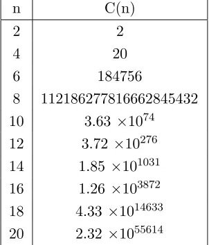
Denote by C(n) the number of balanced majority functions. Then C(n) = 00
= 1 for any odd value n. Whennis even, it is easy to prove that
C(n) =
n n/2 n n/2 /2 ! .
From table 1 it can be seen that the size of C(n) increases very fast with the increase ofn.
For the general case, by Stirling formula: n!≈√2πnn+21e−n+ 1
12n, we can get an
approx-imation: n n/2 ! ≈ 2 n+1 q
2nπe41n
≈ 2
n+1 √
2nπ
and hence
C(n) =
n n/2 n n/2 /2 !
≈22
n+1
√
2nπ− n
2+ 1
4n14π−14e81n
n C(n)
2 2
4 20
6 184756
8 112186277816662845432
10 3.63×1074
12 3.72×10276
14 1.85×101031
16 1.26×103872
18 4.33 ×1014633 20 2.32 ×1055614
Table 1: The number of balanced majority functions in even number of variables
5.2 The Walsh spectrum characterization
Since the definition of majority functions differs much for the cases whennis odd and when
nis even, our discussion will treat each of the cases respectively. Note that, when we write the XOR of two vectors such as x⊕s, it means the bit-wise XOR of vectors x and s. In particular, x⊕1 means the complement of x, i.e., all the coordinates of x is taken the complement by XORing with 1.
5.2.1 When n is odd:
First we notice the following property of this class of functions:
Theorem 2 When n is odd, a Boolean function f(x) defined in definition 3 satisfies:
f(x⊕1) =f(x)⊕1.
Proof: By definition 3, f(x) = 0⇐⇒ WH(x)≤(n−1)/2 ⇐⇒ WH(x⊕1)≥(n+ 1)/2
⇐⇒ f(x⊕1) = 1. Similarly, f(x) = 1 ⇐⇒f(x⊕1) = 0. 2
Theorem 3 Let f(x) be a majority function in n variables, where n is an odd number, then the Walsh transform of f(x) satisfies:
S(f)(w) =
0, if WH(w) is even;
2 P
WH(x)≤n−21
(−1)w·x, if W
H(w) is odd. (31)
Proof: Since f(x) is a majority function in odd number of variables, we have
S(f)(w) = X
x∈GFn(2)
= X WH(x)≤n−21
(−1)w·x− X WH(x)≥n+12
(−1)w·x
= X
WH(x)≤n−21
(−1)w·x− X
WH(x)≤n−21
(−1)w·(1⊕x)
= X
WH(x)≤n−21
(−1)w·x− X WH(x)≤n−21
(−1)w·1+w·x
= X
WH(x)≤n−21
(−1)w·x− X
WH(x)≤n−21
(−1)WH(w)+w·x
=
0, ifWH(w) is even;
2 P
WH(x)≤n−21
(−1)w·x, ifWH(w) is odd.
2
It is noted that when n is even, all the majority functions are symmetric, and in this case, a more convenient Walsh characterization is to treat input with different Hamming weight, and such a characterization can be found in [3].
5.2.2 When n is even:
Since the loose majority functions and the strict majority functions are both symmetric, their Walsh spectrum characterization can be done by treating the difference of the Ham-ming weight of the input, and such characterization can be found in [3] as well.
However in the general case, since set majority functions are not symmetric, Walsh spectrum characterization in terms of different Hamming weight of the inputs makes no sense, so we treat individual inputs. From definition 4 it is known that the majority function in even number of variables is not uniquely determined, it depends on the set A. Denote by A0 =S\A={x:x∈S and x6∈A} to be the complement set of A with respect to S,
and define
A1 = {x:x∈GFn(2) andWH(x)< n
2}
A2 = {x:x∈GFn(2) andWH(x)> n
2}
A3 = {x:x∈A\(A∩A¯)}
A4 = {x:x∈A0\(A0∩A¯0)}
A5 = {x:x∈A∩A¯}
A6 = {x:x∈A0∩A¯0}
where ¯A={x⊕1: x∈A}. Then it is easy to prove the following:
Lemma 2 The above defined sets satisfy the following:
2. f(x)|A1 = 0, f(x)|A2 = 1, f(x)|A3 = 0, f(x)|A4 = 1, f(x)|A5 = 0, f(x)|A6 = 1, where
f(x)|Arepresents the constraint function off(x)whose variablexcan only take values
from A.
3. Define a mapφ(x) =x⊕1. It maps every coordinate of x to its complement, and for a set B ⊂GFn(2), we denote φ(B) ={y=φ(x) : x∈B}. Then we have φ2(x) =x,
φ2(B) =B, and φ(A1) =A2, φ(A3) =A4,φ(A5) =A5,φ(A6) =A6.
Based on lemma 2, we can formulate the Walsh transform of the majority functions in even number of variables. First we give
Lemma 3 Let V ⊂GFn(2)be a self-complement set, i.e. V¯ ={x⊕1: x∈V}=V, then for any odd Hamming weight vector w∈GFn(2), we have P
x∈V
(−1)w·x= 0.
Proof: Denote U = P x∈V
(−1)w·x, then
U = P
x∈V
(−1)w.(x⊕1)
= P
x∈V
(−1)w·x+WH(w)
= (−1)WH(w) P x∈V
(−1)w·x (SinceWH(w) is odd)
= −U.
Hence U = 0. 2
Theorem 4 Let fA(x) be a majority function in n variables. Then the Walsh transform
of fA(x) is:
S(fA)(w) =
P x∈A5
(−1)w·x− P x∈A6
(−1)w·x, if W
H(w) is even;
2 P
x∈A3 or WH(x)<n2
(−1)w·x, ifWH(w) is odd. (32)
Proof: By the definition of fA(x) with respect to the sets A and S, and note that S =A∪A0 =A3∪A5∪A4∪A6 and GFn(2) =S∪A
1∪A2 =S6i=1Ai, by lemma 2 and
lemma 3 we have
S(fA)(w) = X
x∈GFn(2)
(−1)fA(x)+w·x
= X
x∈A1
(−1)w·x− X
x∈A2
(−1)w·x+ X
x∈A3
(−1)w·x− X
x∈A4
(−1)w·x
+ X
x∈A5
(−1)w·x− X
x∈A6
(−1)w·x
= X
x∈A1
(−1)w·x− X
x∈A1
(−1)w·(x⊕1)+ X
x∈A3
(−1)w·x− X
x∈A3
+ X x∈A5
(−1)w·x− X x∈A6
(−1)w·x
= X
x∈A1
(−1)w·x−(−1)WH(w) X
x∈A1
(−1)w·x
+ X
x∈A3
(−1)w·x−(−1)WH(w) X
x∈A3
(−1)w·x
+ X
x∈A5
(−1)w·x− X
x∈A6
(−1)w·x
=
P x∈A5
(−1)w·x− P x∈A6
(−1)w·x, ifW
H(w) is even;
2 P
x∈A1∪A3
(−1)w·x, ifW
H(w) is odd
=
P x∈A5
(−1)w·x− P x∈A6
(−1)w·x, ifWH(w) is even;
2 P
x∈A3orWH(x)<n2
(−1)w·x, ifWH(w) is odd
2
6
On the non-correlation immunity of majority functions
In order to check if the majority functions are correlation immune of any order at all, we might first look at whether they are correlation immune of order 1, for this purpose, by Lemma 1, we only need to verify their Walsh spectrum on a vector w with Hamming weight 1. Without loss of generality, let the vectorei, as defined before, be such whosei-th
coordinate is 1 and 0 elsewhere.
Regarding the correlation immunity of majority functions, we have the following conclu-sion.
Theorem 5 No of the majority functions defined in definition 3 and definition 4 is corre-lation immune.
Proof: Item 3 of Lemma 4 in [3] and Lemma 1 has shown that all symmetric majority functions are not correlation immune of order 1, this includes all the majority functions in odd number of variables, and the loose majority and the strict majority function in even number of variables. So we only need to show that the set majority functions in even number of variables in the general case are also not correlation immune of order 1.
Whenn is even, by theorem 4 we have
S(fA)(ei) = 2 X
x∈A1∪A3
(−1)ei·x= 2[ X
WH(x)<n2
(−1)xi+ X
x∈A3
(−1)xi]
Among all the n-dimensional vectors x with WH(x) < n2, the number of such vectors
that also satisfy that the i-th coordinate is 1 (and the other n−1 coordinates can have 0∼ n2 −1 of 1’s) is
n−1 0
!
+ n−1 1
!
+ n−1 2
!
+· · ·+ nn−1
2 −1
and the number of such vectors whosei-th coordinate is 0 (and the othern−1 coordinates can have 0∼ n−21 of 1’s) is
n−1 0
!
+ n−1 1
!
+ n−1 2
!
+· · ·+ n−n 1
2
! .
Therefore
X
WH(x)<n2
(−1)xi = ( n−1
0
!
+ n−1 1
!
+ n−1 2
!
+· · ·+ n−n 1
2
!
)
−( n−1 0
!
+ n−1 1
!
+ n−1 2
!
+· · ·+ nn−1
2 −1
!
)
= n−n 1
2
!
therefore we have
S(fA)(ei) = 2[
n−1
n
2 −1
!
+ X
x∈A3
(−1)xi].
We show that the above is not always zero, i.e., if the above is zero for some i, then there must exist j such that S(fA)(wj) 6= 0. Denote by A
i1
3 = {x ∈ A3 : xi = 1} and
Ai30 ={x∈A3: xi = 0}, then A3 =Ai30∪Ai31.
Assume for somei,S(fA)(ei) = 0, then P x∈A3
(−1)xi = 1− n−1 n
2−1
.This means that|Ai31| −
|Ai30|= nn−1
2−1
−1. Note that when thei-th coordinate is fixed to be 1, the number of such vectors in S is nn−1
2−1
(the other n−1 coordinates has n2 −1 of 1’s). Since |Ai1
3 | cannot
be larger than nn−1
2−1
, then there are only two cases: (1) |Ai31| = nn−1
2−1
and |Ai30| = 1; or
(2) |Ai31|= nn−1
2−1
−1. We show that in both of the cases, there must exist a j such that
S(fA)(wj)6= 0 and hence induces the conclusion of the theorem.
If case (1) is true, then the othern−1 coordinates (except i) of the vectors in A3 have
all the possible vectors of Hamming weight n2−1. So for anyj 6=i, there are nn−2
2−1
elements in Ai31 whose j-th coordinate is 0 (let the other n−2 coordinates take n2 −1 of 1’s), and there are nn−2
2−2
elements inAi1
3 whosej-th coordinate is 1 (let the other n−2 coordinates
take n2 −2 of 1’s). Since the j-th coordinate of the element inAi30 may be 0 or 1, we have
X
x∈A3
(−1)xj = n−2
n
2 −1
!
− nn−2
2 −2
!
−c= n(n−2)!
2!(n2 −1)! −c,
where c∈ {0,1}, which is larger than or equals to 0 when n >2, and hence S(fA)(wj)>0.
If case (2) is true, then similarly othern−1 coordinates (excepti) have all but one of the possible vectors of Hamming weight n2 −1. So for any j6=i, there are nn−2
2−1
−c1 elements
in Ai31 whosej-th coordinate is 0 (let the other n−2 coordinates take n2 −1 of 1’s, taking away one such vector), and there are nn−2
2−2
−c2 elements in Ai31 whosej-th coordinate is 1
(let the othern−2 coordinates take n2 −2 of 1’s, taking away one such vector). Hence we have
X
x∈A3
(−1)xj = n−2
n
2 −1
!
−c1−[
n−2
n
2 −2
!
−c2] =
(n−2)!
n
2!(n2 −1)!
where c1, c2 ∈ {0,1}. As in case (1), when n >2, it results inS(fA)(wj)>0. Whenn= 2,
all the possible majority functions in 2 variables are: f1(x) =x1,f2(x) =x2,f3(x) =x1x2
and f4(x) = x1⊕x2⊕x1x2. It is easy to verify that no of these functions is correlation
immune, and hence the conclusion of the theorem is true. 2
7
On the fractional correlation immunity of majority
func-tions
Given the Walsh characterization of the fractional correlation immunity and the Walsh spectrum characterization of majority functions, it is easy to link the two together to give an explicit description on the fractional correlation immunity of majority functions. Let
f(x) be the majority function innvariables being considered.
7.1 When n is odd
By definition 3 it is known that, f(x) = 1 if and only if WH(x) ≥ n+12 . Similar to the discussion above, among the vectors with Hamming weight being larger than or equals to
n+1
2 , the number of such vectors where thei-th coordinate is 0 (and the restn−1 coordinates
can have n+12 ∼n−1 of 1’s) is nn−−11
+ nn−−12
+· · ·+ nn−+11 2
, and the number of such vectors where the i-th coordinate is 1 (and the restn−1 coordinates can have n−21 ∼n−1 of 1’s) is nn−−11
+ nn−−12
+· · ·+ nn−−11
2
. Therefore
S(f)(ei) = −2
X
x∈supp(f)
(−1)xi
= 2[ n−1
n−1
!
+ n−1
n−2
!
+· · ·+ nn−−11
2
!
]
−2[ n−1
n−1
!
+ n−1
n−2
!
+· · ·+ nn−+11
2
!
]
= 2 nn−−11
2
!
Note that here the value of S(f)(ei) is independent of i, hence by Eqn. (22) we have
F CI(f) = 1− 1 2WH(f)
max
i |S(f)(ei)|
= 1− 1
WH(f)
. nn−−11
2
!
(33)
By definition 3 we know that, when nis odd, the majority functions are balanced, i.e.,
WH(f) = 2n−1, and hence the above becomes
F CI(f) = 1− 1 2n−1
n−1
n−1 2
By Stirling formula: n!≈√2πnn+12e−n+ 1
12n, we further have
n n
2
!
= n! (n2)2 ≈
√
2πnn+12e−n+121n
2π(n2)n+1e−n+31n =
2n+1e−1 4n
√
2nπ
Then
n−1
n−1 2
!
≈ 2
n
p
2π(n−1)e
−4(n1−1)
So
1− 1
2n−1
n−1
n−1 2
!
≈1−
s
2
π(n−1)e
−4(n1−1) ≈1−
s
2
π(n−1).
Summarize the discussion above, we have
Theorem 6 When n is odd, the fractional correlation immunity of the majority functions is
F CI(f) = 1− 1 2n−1
n−1
n−1 2
!
≈1−
s
2
π(n−1). (34)
7.2 When n is even
By theorem 4 we have
S(fA)(ei) = 2
X
x∈A3orWH(x)<n2
(−1)ei·x = 2[X
x∈A3
(−1)xi+ X
WH(x)<n2
(−1)xi].
It is easy to verify that, among then-dimensional vectors of Hamming weight less than n2, the number of such vectors where the i-th coordinate is 0 (and the restn−1 coordinates can have 0∼(n2 −1) of 1’s) is n−01
+ n−11
+· · ·+ nn−1
2−1
, and the number of such vectors where the i-th coordinate is 1 (and the rest n−1 coordinates can have 0∼ n2 −2 of 1’s) is
n−1 0
+ n−11
+· · ·+ nn−1
2−2
. Therefore
X
WH(x)<n2
(−1)xi = [ n−1
0
!
+ n−1 1
!
+· · ·+ nn−1
2 −1
!
]
−[ n−1 0
!
+ n−1
1
!
+· · ·+ nn−1
2 −2
!
]
= nn−1
2 −1
! .
Note from the definition that|S|= nn
2
andA3 cannot have more than half of the elements
inS(otherwiseA3 would have at least a pair of complement vectors which contradicts with
its definition), i.e. |A3| ≤ |S2| = nn
2
/2. Since
−|A3| ≤ X
x∈A3
so we get a lower bound of S(fA)(ei):
S(fA)(ei) ≥ 2[−|A3| −
n−1
n
2 −1
!
]
≥ 2[− nn
2
!
/2− nn−1
2 −1
!
]
= −2 nn
2
!
and an upper bound
S(fA)(ei) = 2[|A3| −
n−1
n
2 −1
!
]
≤ 2[ nn
2
!
/2− nn−1
2 −1
!
]
= 0.
By definition 4, we have
WH(fA) =
n n
2 + 1
!
+ nn
2 + 2
!
+· · ·+ n
n !
+|A3|
≥ nn
2 + 1
!
+ nn
2 + 2
!
+· · ·+ n
n !
= 2n−1− nn
2
! /2.
Therefore, by Eqn. (22) we have
F CI(fA) = 1−
1 2WH(fA)
max
i |S(fA)(ei)|
≥ 1− 2
2n− nn
2
. nn
2
!
≈ 1−√ 4
2nπ−2.
Summarize the discussion above we have
Theorem 7 When n is even, then the fractional correlation immunity of any majority function fA(x) in n variables satisfies
F CI(fA)≥1−
2 2n− nn
2
n n
2
!
≈1−√ 4
2nπ−2. (35)
Noticing that whennis odd, by theorem 6 we have
lim
n→∞F CI(f) = 1,
and when nis even, by theorem 7 we have
lim
n→∞F CI(fA) = 1,
Theorem 8 The fractional correlation immunity of the majority functions defined in defi-nition 3 and defidefi-nition 4 approaches to 1 with the increase of the number of variables.
Theorem 8 means that the majority functions are almost correlation immune, and they are more close to being correlation immune with the increase ofn. This asymptotic property is called approaching correlation immunity.
8
Concluding remarks
This paper proposed a new security measure of cryptographic Boolean functions called fractional correlation immunity. When the fractional correlation immunity reaches value 1, it is the correlation immunity in the traditional sense. How the new measure is related to the resistance against correlation attack when such a function is used as the combining function in a nonlinear combiner is studied.
This paper also studies the fractional correlation immunity of majority functions. It is shown that for the correlation immunity in the traditional sense, no majority function is correlation immune. However the fractional correlation immunity of majority functions approaches to 1 with the number of variables grows. This means that the majority logic functions also have good resistance against correlation attack.
It is noted that the results in this paper can be generalized to the case ofk-order fractional correlation immunity, where the analysis is unavoidably more complicated. It should be pointed out that the concept of fractional correlation immunity can also be used to study other classes of Boolean functions.
References
1. A. Braeken and B. Preneel: “On the Algebraic Immunity of Symmetric Boolean Functions”, In Progress in Cryptology - INDOCRYPT 2005, LNCS 3797, Springer-Verlag 2005, pp.35-48.
2. A. Canteaut and M. Videau: “Symmetric Boolean functions”,IEEE Trans. on Infor-mation Theory, Vol. IT-51, No.8, 2005, pp.2791-2811.
3. D. K. Dalai, S. Maitra and S. Sarkar: “Basic theory in construction of Boolean func-tions with maximum possible annihilator immunity”,Design Codes and Cryptography, Vol.40, No.1, 2006, pp.41-58.
4. N. Li and W.-F. Qi: “Symmetric Boolean functions depending on an odd number of variables with maximum algebraic immunity”,IEEE Trans. on Information Theory, Vol.IT-52, No.5, 2006, pp.2271-2273.
functions”, In Advances in Cryptology-EUROCRYPT 2004, LNCS 3027, Springer-Verlag 2004, pp.474-491.
6. T.Siegenthaler: “Correlation-immunity of nonlinear combining functions for crypto-graphic applications”, IEEE Trans. on Information Theory, Vol. IT-30, No.5, 1984, pp.776-780.
7. T. Siegenthaler: “Decrypting a Class of Stream Ciphers Using Ciphertext Only”,
IEEE Trans. on Computers, Vol.C-34, No.1, 1985, pp81-85.
8. C.K.Wu, X.Wang: “Balanced source coding and its applications in stream ciphers”,
ACTA Electronica Sinica, Vol.21, No.7, 1993, pp.23-32 (in Chinese).