Enhanced TWI under Wall Parameter Uncertainty with the
Parametric Sparse Recovery Method
Fangfang Wang1, 2, *, Huiying Wu1, and Tingting Qin1
Abstract—In recent years, through-wall imaging (TWI) has gained much research interest because of urgent needs of civilian, security, and defense applications. TWI based on compressive sensing (CS) method can produce high resolution, assuming that the wall parameters are known in prior. However, it is difficult to know the exact wall parameters in actual scenarios. With unknown wall parameters, the dictionary matrix is not a fixed one. Therefore, CS theory cannot be directly applied in the TWI. This paper presents a parametric sparse recovery method for TWI with unknown wall parameters. The original reconstruction problem is reformulated into a joint optimization one which can be solved with an alternating minimization algorithm. Specifically, the proposed method performs the wall parameter estimation and sparse image reconstruction in an iterative procedure. With the estimated wall parameter which is or close to the true one, the high fidelity and high-resolution image is obtained. Experimental simulations show that the proposed method can obtain an autofocus image and improve the image quality.
1. INTRODUCTION
Sensing through obstacles such as walls, doors, and other visually opaque materials using microwave signal is emerging as a powerful tool to support a range of civilian and military applications [1]. Through-wall imaging (TWI) is an emerging technology that allows noninvasive surveys of the region of interest behind the front wall by providing high-resolution images [2, 3].
High-resolution imaging demands large bandwidth signals and a large array aperture. The Shannon’s celebrated theorem requires that the signal is sampled at a frequency not lower than twice its bandwidth. Therefore, the application of some traditional techniques to TWI system is usually severely constrained by this Nyquist’s sampling rate.
The new emerging theory of compressive sensing (CS) provides an idea to overcome the restriction in data acquisition based on the Shannon’s theorem and to allow one to recover signals from far fewer measurements than traditional techniques [4]. The signal reconstruction in the framework of CS is guaranteed by two requirements: sparsity and incoherency [5]. Sparsity implies that most elements of the signal are zero, which is a necessary prior assumption in most cases. Making use of the sparsity of the scene, CS was widely applied in radar imaging, providing an efficient way of high-resolution image reconstruction using few frequency and spatial observations [6].
CS is firstly applied to radar imaging by Baraniuk and Steeghs [7]. The application of this innovative technology can avoid the usage of an expensive receiving A/D converter, therefore simplifying the radar imaging system. A high-resolution TWI method with CS is firstly presented by Yoon and Amin, and a Fourier-like measurement matrix is designed to reduce sampled data in frequency domain [8]. Also, a non-adaptive randomized projection is proposed when through-wall imaging based on CS method is
Received 26 July 2019, Accepted 17 October 2019, Scheduled 2 November 2019 * Corresponding author: Fangfang Wang (wangff@njupt.edu.cn).
1 School of Electronic Science and Engineering, Nanjing University of Posts and Telecommunications, Nanjing 210003, China. 2
used [9]. This method can obtain low side-lobe images even with high noise, and 7.7% of measurement data is enough to recover the image. Lately, Leigsnering et al. analysed the pronounced multipath phenomenon due to walls, ceilings, and floors surrounding the targets of interest and combined the multipath exploitation and compressive sensing to achieve a good image reconstruction in multipath environments from far fewer spatial and frequency measurements [10–12].
The CS based TWI procedure consists of three parts: building a dictionary, performing measurement, and solving a convex optimization problem. As a result, the construction of dictionary directly determines the performance of imaging. It is noted that the dictionary is related to all factors or parameters of a radar system and background. In traditional application of CS, these parameters are supposed to be known a prior. Thus, it is easy to construct the dictionary using either an analytical or numerical approach. However, it is difficult to acquire these parameters, and thus the dictionary is not a pre-design matrix, so CS theory cannot be directly applied. As an alternative approach, parametric sparse representation model containing unknown parameters is constructed which leads to a joint optimization problem to simultaneously solve image reconstruction and parameter estimation [13]. The “maximum contrast search” method combining with matching pursuit (MP) is proposed for inverse synthetic aperture radar (ISAR) 2-D imaging of uniformly rotating targets with an unknown rotation rate in the framework of parametric sparse representation [14]. Imaging reconstructions are performed on dictionary candidates of preselected rotation rate, and the exact rotation rate is determined when the corresponding image contrast reaches the maximum. Meanwhile, the image according to the estimated rotation rate is the output of the result. Nevertheless, this method is time-consuming because of repeating the same imaging process for all candidates. To improve the imaging efficiency and reduce computational burden, an iterative framework is proposed in [15]. This method includes two alternative steps: updating the new ISAR imaging by weighted l1 minimization and correcting the rotation rate
by least square (LS) method. The iteration will stop until the parameter error is less than a designated threshold.
It is noted that the proposed parametric sparse representation approach is also applicable to imaging through unknown walls [16]. In this work, a parametric dictionary with an unknown wall parameter is designed to represent the wall’s ambiguity. Therefore, the original problem is reformulated into a joint optimization one which is solved in an iterative manner. The proposed method can estimate the best wall parameter by nonlinear optimization method and recover the sparse signal with orthogonal matching pursuit (OMP) in an iterative framework. Toward this end, LS and conjugate gradient (CG) method are used for the nonlinear optimization respectively. With the best wall parameter, the high-resolution image is obtained by OMP algorithm.
The remainder of this paper is organized as follows. Section 2 presents the signal model in the framework of typical CS and parametric sparse representation. In the framework of parametric sparse representation, two alternating minimization algorithms are introduced to deal with TWI in the presence of wall parameter uncertainties in Section 3. Section 4 provides some numerical examples, and the paper concludes in Section 5.
2. SIGNAL MODEL
A mono-static synthetic aperture radar (SAR) system is used in this work. Suppose that a UWB impulse radar system with one antenna placed near the wall illuminates the scene by transmitting a wideband Gaussian pulses(t). Meanwhile, the scattered field consisting of M time samples is collected at the same location of the source. Then, the antenna moves parallel to the wall and synthesizes anN
element aperture. Under this operation, themth time sample ofP targets received at thenth synthetic aperture location can be expressed as
z(m, n) =
P−1
p=0
σps(tm−τnp) (1)
thepth target and then to the nth receiver location. It can be approximated by
τnp= 2
(xn−xp)2+ (yn−yp)2
c +
2d
(xn−xp)2+ (yn−yp)2 |yn−yp|c (
√
εr−1) (2)
where (xn, yn) and (xp, yp) are coordinates of thenth synthetic aperture location andpth target location;
c is the velocity of light in the air;dand εr are wall’s thickness and relative permittivity.
The target space behind the wall is partitioned into rectangular cells, with K pixels along the cross-range and Lpixels along the down-range. Then, the target return is given by
z(m, n) =
K,L
k, l=1
σ(k, l)s(tm−τn,(k, l)) (3)
where σ(k, l) = σp if a target exists at the (k, l) pixel, otherwise σ(k, l) = 0. τn,(k, l) is the round-trip
propagation delay of the signal from the nth transmitter location to the (k, l) pixel and then to the
nth receiver location. All measurements z(m, n) are stacked into a single column vector to obtain the measurement data vector.
z= [z(1,1),· · · , z(M,1),· · · , z(M, N)]T (4) As such, Equation (3) can be formally expressed as
z=Ψx (5)
In Eq. (5), Ψ is the matrix that relates the unknown vector to the data vector, and it represents the dictionary under the framework of sparse representation. The (i, j) element ofΨis given by
[Ψ]ij =s(tm−τn,(k, l)) (6)
form=imodM,n=i/M,k=j modK, and l=j/K, mod represents modulo function, and represents floor function. x= [σ1,1,· · · , σK, L]T is the scene reflectivity vector.
2.1. Typical CS Model
In CS scheme, Φis a J×M N measurement matrix to reduce the computational cost, which has only one nonzero element in each row. Here J represents the observation number. All sampled data are randomly projected onto this measurement matrix to obtain the limited observation, which is written as
y=Φz+w (7)
where w is the additive noise, and y is a J ×1 vector. The relationship between the observation and sparse signal can be formalized as
y=ΦΨx+w (8)
2.2. Parametric Sparse Representation Model
Taking a physical perspective, there are many factors and parameters that influence the formation of dictionary Ψ. Any uncertainties of these factors will lead to dictionary mismatch, which may degrade the performance of existing sparsity-based algorithms.
For through-wall radar signal model, each column of the dictionary can be treated as a time shift of the transmitting signal. Obviously, the wall parameters play an important role in the calculation of the time shift when signals propagate through walls. Therefore, the presence of wall ambiguity will bring in the error of the signal model. In what follows, the parametric sparse representation model is proposed to consider the unknown wall parameters. In this paper, only the thickness of walls is assumed to be unknown, so the dictionary can be expressed asΨ(d). Then, the parametric sparse representation model for TWI under wall parameter uncertainty is formulate as
3. PROPOSED ALGORITHM
The parametric sparse representation for signal model shown in Eq. (9) is different from typical CS in that its dictionary is not a predesigned matrix. Because of the unknown parameter d appears in the dictionary matrix, the original problem cannot be solved using some conventional CS algorithms directly. Thanks to the exploitation of parametric sparse representation formation, the problem can be reformulated into a joint one
ˆ
d,xˆ
= arg min
{d,x}
x1+λy−ΦΨ(d)x22
(10)
where λ is a regularization parameter. To properly address such a joint issue, the alternating minimization algorithm is applied. Specifically, the alternating iterative procedure can be realized by alternatively solving two sub-problems, i.e., “x sub-problem” and “d sub-problem”. Actually, it turns out that “xsub-problem” can be directly solved by OMP method when dis fixed. On the other hand, since “dsub-problem” is a nonlinear one, LS and CG approaches are used to solve the nonlinear optimization problem in this paper.
3.1. OMP Combined with LS
The fundamental idea of this alternating iterative algorithm is to update the wall parameterd(i+1) with the LS approach and to update the sparse solution x(i+1) with OMP. More specifically, the iterative step-size Δd of the wall parameter is calculated with the LS method by taking the first-order Taylor expansion of the dictionary. The iteration will stop until step-size Δdis less than a preset thresholdγ. The detailed steps flow is outlined as follows:
Initialization: initialize the iteration indexi= 0 and the wall parameterd(0)
Step 1: Construct the dictionary Ψ(d(i)) and update the sparse solution, such that
x(i+1)= arg min
x
x1+λy−ΦΨ
d(i) x2
2
(11)
Step 2: Update the wall parameter, such that
d(i+1)= arg min
d
y−ΦΨ(d)x(i+1)2
2 (12)
Step 3: Update the iteration indexi←i+ 1, and repeat steps 1–2 until a suitable stopping criterion is satisfied. The iteration will stop if step-size Δdis less than a preset threshold γ.
For updating the wall parameter in Step 2, Ψ(d) can be expanded in d(i) using the first-order Taylor expansion as
Ψ(d) =Ψ
d(i) + ∂Ψ
∂d
d=d(i)
Δd (13)
Thus update ofdis cast into update of Δd, which is formulated as
Δd= arg min
Δd
y−ΦΨ
d(i) ·x(i+1)−Φ ∂Ψ(d)
∂d
d=d(i)
·x(i+1)·Δd
2
2
(14)
Then Δdis calculated by the LS method which is expressed as
Δd =
Φ∂Ψ(d)
∂d
d=d(i)
·x(i+1)
T
·
Φ∂Ψ(d)
∂d
d=d(i)
·x(i+1)
−1
·
Φ∂Ψ(d)
∂d
d=d(i)
·x(i+1)
T
y−ΦΨ
d(i) ·x(i+1) (15)
3.2. OMP Combined with CG
In this alternating iterative procedure, the conjugate gradient approach is applied to solve “d sub-problem”, and the OMP is used to solve “xsub-problem”. A data misfit function H(d) is constructed to denote the recovery error
H(d) =y−ΦΨ(d)x22 (16) The detailed steps flow of this algorithm is outlined as follows:
Step 1 Outer loop (Outer loop initialization): Initialize the iteration index i = 0 and the wall parameterd(0)
Step 2 Outer loop (Sparse reconstruction): Construct the dictionary Ψ(d(i)), and update the
sparse solution, such that
x(i+1)= arg min
x
x1+λy−ΦΨ
d(i) x2
2
(17)
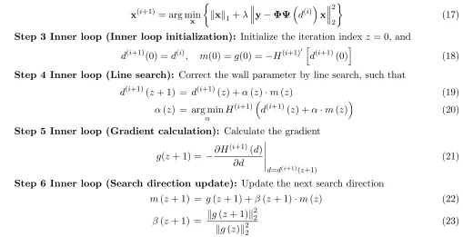
Step 3 Inner loop (Inner loop initialization): Initialize the iteration indexz= 0, and
d(i+1)(0) =d(i), m(0) =g(0) =−H(i+1)
d(i+1)(0)
(18)
Step 4 Inner loop (Line search): Correct the wall parameter by line search, such that
d(i+1)(z+ 1) = d(i+1)(z) +α(z)·m(z) (19)
α(z) = arg min
α
H(i+1)
d(i+1)(z) +α·m(z) (20)
Step 5 Inner loop (Gradient calculation): Calculate the gradient
g(z+ 1) = −∂H
(i+1)(d)
∂d
d=d(i+1)(z+1)
(21)
Step 6 Inner loop (Search direction update): Update the next search direction
m(z+ 1) = g(z+ 1) +β(z+ 1)·m(z) (22)
β(z+ 1) = g(z+ 1)
2 2
g(z)22 (23)
Step 7 Inner loop (Inner loop iteration update): Let z ← z+ 1, and return to Step 4. The iteration will stop until d(i+1)−d(i)22/d(i)22 is less than a pre-set thresholdγ.
Step 8 Outer loop (Outer loop iteration update): Update the iteration index i ← i+ 1, and return to Step 2. The iteration will stop if x(i+1)−x(i)22/x(i)22 is less than a pre-set threshold η.
4. RESULTS
This section is devoted to the assessment of accuracy and robustness when dealing with single or multiple targets in noiseless and noisy conditions. Fig. 1 shows a through wall radar scenario as reference. A synthetic aperture radar scans the scenario along the x-axis positive direction while transmitting a Gaussian pulse s(t). The antenna moves from R1(−1 m,−0.3 m) with spacing of Δr = 0.1 m to
synthesize an aperture of N = 21 radar locations. A target is located behind the wall. The wall thickness, conductivity, and relative permittivity are 15 cm, 0.003 S/m, and 7.66 in finite-different time-domain (FDTD) simulation, respectively. The imaging area BCDE [−2,2]×[0.2,4.2] m2 is equally divided into 41×41 pixels.
The Gaussian pulse s(t) is expressed as
s(t) = sin (2πf0t) exp
−4π(t−t0)
2
T2 p
Figure 1. Geometrical configuration of the problem.
Figure 2. B-scan image for target scattering fields.
where f0 is the central frequency, and Tp is the pulse width. The peak of pulse appears at t0. In
this paper, f0 = 2 GHz, Tp = 1.125 ns, and t0 = 1.125 ns. The scenario is simulated using FDTD and
sampled with M = 2500 measurements at every antenna location. Fig. 2 is the B-scan image for the target scattered fields at each antenna location. It is noted that the total measurement isM N = 52500, and 10% of measurement is used for wall parameter estimation and image reconstruction.
4.1. Simulation Results by OMP Combined with LS Approach
The term in the first-Taylor expansion of dictionary ∂Ψ∂d is related to ∂[s(t−∂dτnp(d))], which is derived as
∂[s(t−τnp(d))]
∂d =
∂
sin (2πf0(t−τnp(d)))·exp
−4π(t−t0−τnp(d))
2
T2 p
∂d
= [sin (2πf0(t−τnp(d)))]·exp
−4π(t−t0−τnp(d))
2
T2 p
+ sin (2πf0(t−τnp(d)))
exp
−4π(t−t0−τnp(d))
2
T2 p
=−(2πf0) cos (2πf0(t−τnp(d)))·
2εr−sin2θ−cosθ
c
·exp
−4π(t−t0−τnp(d))
2
T2 p
+ sin (2πf0(t−τnp(d)))
·exp
−4π(t−t0−τnp(d))
2
T2 p
·8π·(t−t0−τnp(d)) T2
p
·2
εr−sin2θ−cosθ
c (25)
initial wall parameter. To find the best wall thickness, the image contrast Cx(d) is defined as
Cx(d) = 1
N
[x(d)]2
1
N
x(d)
2 (26)
where x(d) represents image related to wall parameter d, and N is the number of pixels. The image contrast is a parameter which evaluates the fluctuation around the mean pixel. The more the autofocus of the image is, the larger the value of image contrast is obtained.
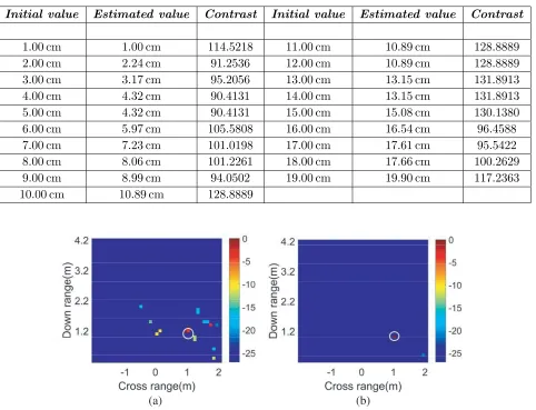
The first set of numerical experiments is aimed at evaluating the effectiveness of this approach. In this simulation, the initial value of wall thickness varies from 1 cm to 20 cm with spacing of 1 cm. Table 1 shows the estimated value of wall thickness and corresponding image contrast with different initial wall parameters when one target is located in the scene. It is clear that the best thickness is 13.15 cm, which is close to the true value. It is noted that there is still a deviation between the estimated and true values due to the model mismatch error. Fig. 3(a) is the reconstructed image of single target without compensation of the wall effect (i.e., equal to free space imaging). The performance significantly degrades and leads
Table 1. The estimated value and corresponding image contrast with different initial wall thickness for a single target.
Initial value Estimated value Contrast Initial value Estimated value Contrast
1.00 cm 1.00 cm 114.5218 11.00 cm 10.89 cm 128.8889
2.00 cm 2.24 cm 91.2536 12.00 cm 10.89 cm 128.8889
3.00 cm 3.17 cm 95.2056 13.00 cm 13.15 cm 131.8913
4.00 cm 4.32 cm 90.4131 14.00 cm 13.15 cm 131.8913
5.00 cm 4.32 cm 90.4131 15.00 cm 15.08 cm 130.1380
6.00 cm 5.97 cm 105.5808 16.00 cm 16.54 cm 96.4588
7.00 cm 7.23 cm 101.0198 17.00 cm 17.61 cm 95.5422
8.00 cm 8.06 cm 101.2261 18.00 cm 17.66 cm 100.2629
9.00 cm 8.99 cm 94.0502 19.00 cm 19.90 cm 117.2363
10.00 cm 10.89 cm 128.8889
(a) (b)
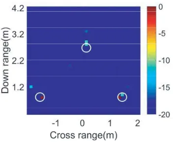
Figure 4. Reconstructed image with OMP combined with LS approach for multiple targets.
to serious false target image. To image accurately, the wall effect should be considered. Fig. 3(b) is the retrieved image after the wall thickness is estimated using the proposed approach. Since the wall delay and compensation have been considered using the estimated wall parameter, the proposed algorithm performs better than the result in Fig. 3(a). It can be seen that well-corrected and well-focused target image can be obtained by the proposed algorithm. Fig. 4 is the restoration of the image with the estimated thickness when multi-targets are located behind the wall. Due to the ignorance of multipath, the farthest target is blurred.
To verify the reliability of the proposed algorithm, the noise is added to the measurements. The signal-to-noise (SNR) is set from 10 dB to 100 dB with an increment of 10 dB. When a single target is considered, the estimated wall thickness is shown in Table 2. Except for SNR = 10 dB, and the estimated wall parameter is still 13.15 cm with other SNR levels.
Table 2. The estimated value for wall thickness with different SNR for a single target.
SNR Estimated value SNR Estimated value
10 dB 13.14 cm 60 dB 13.15 cm 20 dB 13.15 cm 70 dB 13.15 cm 30 dB 13.15 cm 80 dB 13.15 cm 40 dB 13.15 cm 90 dB 13.15 cm 50 dB 13.15 cm 100 dB 13.15 cm
4.2. Simulation Results by OMP Combined with CG Approach
The gradient as illustrated in Eq. (21) is derived as
g=−∂Hi
+1(d)
∂d = 2
y−ΦΨxi+1H ·
Φ·∂Ψ
∂d
·xi+1
d=d(i+1)(z+1)
(27)
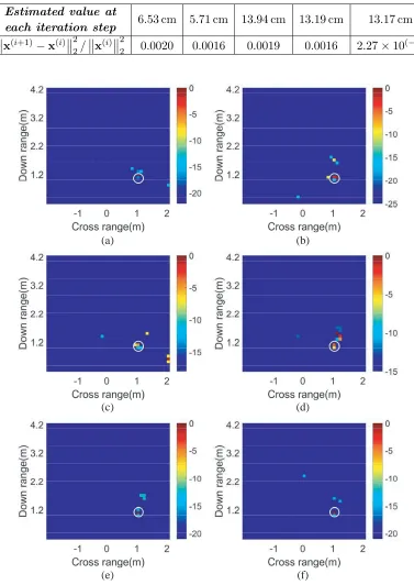
Table 3. The relative error of the reconstructed image at iterations for a single target.
Estimated value at
each iteration step 6.53 cm 5.71 cm 13.94 cm 13.19 cm 13.17 cm
x(i+1)−x(i)2 2/x
(i)2
2 0.0020 0.0016 0.0019 0.0016 2.27×10 (−5)
(a) (b)
(c) (d)
(e) (f)
Figure 5. Reconstructed images at iterations with OMP combined with CG approach: (a) d= 1 cm, (b)d= 6.53 cm, (c) d= 5.71 cm, (d)d= 13.94 cm, (e) d= 13.19 cm, and (f)d= 13.17 cm.
Table 4. The relative error of the reconstructed image at iterations for multiple targets.
Estimated value at
each iteration step 16.05 cm 15.61 cm 15.70 cm 15.62 cm 15.64 cm 15.63 cm
x(i+1)−x(i)2 2/x
(i)2
2 0.0025 0.0014 3.5×10
(−4) 3.0×10(−4) 3.5×10(−4) 2.47×10(−5)
Figure 6. The estimated wall thickness as a function of the iterations for a single target.
Figure 7. The estimated wall thickness as a function of the iterations for multiple targets.
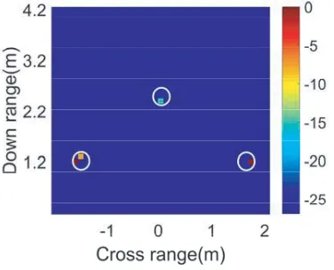
Figure 8. Reconstructed image of multiple targets with OMP combined with CG approach.
5. CONCLUSION
This work presents a parametric sparse recovery method for through-wall imaging with unknown wall thickness. Under the parametric sparse representation framework, the original reconstruction problem for TWI is cast into a joint optimization one. It is difficult to solve the joint optimization problem directly. Two alternating iterative schemes which contain sparse recovery and nonlinear optimization are proposed to estimate the wall thickness and recover the sparse signal simultaneously. In each iteration, OMP is used to achieve the sparse restoration, and two algorithms, LS and CG, are implemented to solve nonlinear optimization.
image contrasts are then compared to find the best wall thickness. The proposed combination methods can enlarge the applicability of compressive sensing to TWI under wall thickness ambiguity. Several numerical results with different numbers of targets and noise conditions have been discussed to analyse the potentialities and features of this iterative scheme in terms of accuracy and robustness to the noise. It is shown that the estimated value for wall thickness is close to the true one, and the corresponding reconstructed image has high fidelity. Moreover, the proposed approach is also suitable for the noisy scenario.
ACKNOWLEDGMENT
This work was supported by the National Natural Science Foundation of China (Grant Nos. 61601245, 61601242), and State Key Laboratory of Millimeter Waves Open Project, Southeast University (Grant No. K201724) and China Postdoctoral Science Foundation Funded Project (Grant No. 2016M601693) and Nanjing University of Posts and Telecommunications Foundation, China (Grant No. NY214047).
REFERENCES
1. Frazier, L. M., “Surveillance through walls and other opaque materials,” Proceedings of the 1996 IEEE National Radar Conference, 1996, 27–31, IEEE, 1995.
2. Song, L. P., C. Yu, and Q. H. Liu, “Through-wall imaging (TWI) by radar: 2-D tomographic results and analyses,” IEEE Transactions on Geoscience & Remote Sensing, Vol. 43, No. 12, 2793–2798, 2005.
3. Amin, M. G., Through-the-wall Radar Imaging, CRC Press, 2011.
4. Massa, A., P. Rocca, and G. Oliveri, “Compressive sensing in electromagnetics — A review,”IEEE Antennas & Propagation Magazine, Vol. 57, No. 1, 224–238, 2015.
5. Donoho, D. L., “Compressed sensing,” IEEE Transactions on Information Theory, Vol. 52, No. 4, 1289–1306, 2006.
6. Herman M. A. and T. Strohmer, “High-resolution radar via compressed sensing,” IEEE Transactions on Signal Processing, Vol. 57, No. 6, 2275–2284, 2009.
7. Baraniuk, R. and P. Steeghs, “Compressive radar imaging,” Radar Conference, 128–133, IEEE, 2007.
8. Yoon, Y. S. and M. G. Amin, “Compressed sensing technique for high-resolution radar imaging,”
SPIE Defense and Security Symposium, International Society for Optics and Photonics, 69681A– 69681A-10, 2008.
9. Huang, Q., L. Qu, B. Wu, et al., “UWB through-wall imaging based on compressive sensing,”IEEE Transactions on Geoscience & Remote Sensing, Vol. 48, No. 3, 1408–1415, 2010.
10. Leigsnering, M., F. Ahmad, M. Amin, et al., “Multipath exploitation in through-the-wall radar imaging using sparse reconstruction,” IEEE Transactions on Aerospace & Electronic Systems, Vol. 50, No. 2, 920–939, 2014.
11. Leigsnering, M., M. Amin, F. Ahmad, et al., “Multipath exploitation and suppression for SAR imaging of building interiors: An overview of recent advances,” IEEE Signal Processing Magazine, Vol. 31, No. 4, 110–119, 2014.
12. Liu, J., L. Kong, X. Yang, et al., “First-order multipath Ghosts’ characteristics and suppression in MIMO through-wall imaging,” IEEE Geoscience & Remote Sensing Letters, Vol. 13, No. 9, 1315–1319, 2016.
13. Chen, Y. C., G. Li, Q. Zhang, et al., “Motion compensation for airborne SAR via parametric sparse representation,” IEEE Transactions on Geoscience& Remote Sensing, Vol. 55, No. 1, 551– 562, 2016.
15. Rao, W., G. Li, X. Wang, et al., “Adaptive sparse recovery by parametric weightedl1 minimization
for ISAR imaging of uniformly rotating targets,”IEEE Journal of Selected Topics in Applied Earth Observations &Remote Sensing, Vol. 6, No. 2, 942–952, 2013.