A STABLE MARCHING-ON-IN-TIME SCHEME FOR WIRE SCATTERERS USING A NEWMARK-BETA FORMULATION
S. E. Bayer
University of Kocaeli
Mechatronic Engineering Department Veziroglu Campus, ˙Izmit, Kocaeli, Turkey
A. A. Ergin
Gebze Institute of Technology Electronic Engineering Department
C¸ ayırova Campus, P.K.: 141,41400 C¸ ayrova, Gebze/Kocaeli, Turkey
1. INTRODUCTION
Nowadays, there is a growing interest in the study of radiation and propagation of transient electromagnetic waves. Numerical methods have very important roles for the analysis of transient electromagnetic scattering problems and may involve both frequency-domain (FD) solutions together with inverse discrete Fourier transform (IDFT) technique to convert the results to time domain or time-domain (TD) solutions by formulating the problem directly in the time-domain using a time-marching algorithm. Most popular time-domain techniques are the method of finite difference in time domain (FDTD) [5] and the method of marching-on-in-time (MOT) [6, 7].
This study aims to increase the stability of the MOT method which was developed to examine scattering of wide-band electromagnetic pulses from objects. In the past, various solutions were suggested to increase the stability of the MOT method such as time or space averaging methods [7–10], good choice of temporal basis functions [11], and the use of combined-field integral equation [1]. However, the solutions in question are either applicable for analysis of scattering from surfaces (for example, [1]) or provide stability by employing artificial signal processing techniques [7–10]. As a result, literature does not contain a special stability analysis and solution suggestion developed for the MOT methods solving the problem of scattering from thin wires.
This study suggests two basic solutions to increase the stability in analysis of scattering from wires. The first solution is the Newmark-Beta formulation which was used in general for the time-domain finite element method (FEM) [12]. This method calculates the derivatives of the terms approximately by using finite differences and uses an independent beta (β) parameter to increase the stability. The second solution examines the contribution of analytic evaluation of some of the integrals, which had been considered in numerical terms to date for the MOT method, to the stability. Numeric errors have been suggested to be one of the reasons of instability in the MOT method [8]. Here the basic hypothesis is that, the integral results calculated analytically will eliminate some of the numeric errors and will contribute to the stability.
2. THE ELECTRIC FIELD INTEGRAL EQUATION (EFIE)
(PEC) scatterer surface is equal to zero. Therefore, we have
∂Eit ∂t =
∂2A ∂t2 +
∂ ∂t∇φ
t
(1)
whereA and φare the magnetic vector and scalar electric potentials, respectively, and Ei denotes the incident electric field. The subscript ‘t’ denotes the tangential components to wire surface. The magnetic vector potential A and scalar potential φ are in the retarded time integral form and are mathematically represented by
A(r, t) =µ
v
J(r, t−R/c) 4πR dv
φ(r, t) = 1
ε
v
ρ(r, t−R/c) 4πR dv
(2) where R = |r−r| represents the distance between the observation point r and source point r, ρ is the charge density, J is the current density,cis the velocity of propagation of electromagnetic wave in the space, µ and ε are the permeability and permittivity of free space, respectively. t−R/c represents the retarded time. In Eq. (1), the incident fieldEitis known and induced current density on the scatterer
J(r, t−R/c) is not known, but it is wanted to be found.
3. SOLUTION OF EFIE FOR THIN-WIRES BY CLASSICAL MOT
In this section the solution of the EFIE for thin wires by the classical MOT method will be outlined.
3.1. Basis Function
When conductors are thin wires (a << λ), the current is assumed to flow only in the wire axis direction ˆ and only along the wire axis. Hence, the unknown current density can be expressed as J(r, t) =
J(, t) = ˆ()I(, t) by using thin wire approximation.
Current density in terms of N spatial basis functions fn(), and temporal basis functionsTi(t) is:
J(, t) =
N
n=1
In(t)fn() = N
n=1
i
In,iTi(t)fn() (3)
Here,In,iare the unknown coefficients,Ti(t) is time basis function and
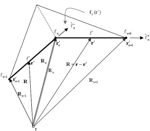
Figure 1. Definition of the basis function.
interval is divided into ∆t equal time steps and T(t) is a quadratic function [13]. The subscript ‘i’ denotes the current on the ith time step is related with basis functions T(t−i∆t). fn() is a linear basis function [14], the parameters related to the spatial basis functionfn() are shown in Fig. 1 and its mathematical expression can be given as
fn() =
−n−1 s−n
ˆ
−n ∈Sn− n+1+
s+n
ˆ
+n ∈Sn+
; n∈ {1, . . . , N} (4)
Here, n means nth node’s coordinate in term of parameter and s±n = |n+1−n|. Also, s−n is wire segment between [n−1, n] points
ands+n is wire segment between [n, n+1] points. Eq. (4) can be written as
fn() =
±n±1− s±n
ˆ
±n n <> <> n±1 (5) For the thin wire case, the EFIE can be written in the form of
∂tEit(, t) =
∂t2A(, t) +∇∂tφ(, t)
t (6)
where ∂t denotes ∂/∂t. After substituting Eq. (3) in (6), so we need
3.2. Testing Procedure
If we apply spatial Galerkin testing at timet=tj to Eq. (6), the result is
fm(), ∂tEi(, t)
t=tj
Emj
= ∂t2fm(),A(, t)
t=tj
ψmj
+fm(),∇∂tφ(, t)
t=tj
varphimj
; m∈ {1, . . . , N}(7)
where f, g inner product is f, g = f()g()d. Eq. (7) can be written as
Em,j =∂2tψm,j+ϕm,j (8)
Since there areN number of basic functions, differentm∈ {1, . . . , N}
values can be used for Eq. (7) in order to write an equation indicating
N number of numeric parities. Second order derivative in Eq. (8) can be implemented with the finite difference method and Eq. (8) can be written in the form
Em,j ∼= ψm,j+1−2ψm,j+ψm,j−1
∆t2 +ϕm,j (9)
approximately. In the inner product expression shown as ψm,j in
Eq. (7), can be written as
ψm,p = fm(),A(, t) t=tp
=
Sm
fm()A(, tp)d (10)
can be expanded by using Eqs. (2), (3) and the result can be shown as
ψm,p = µ
Sm
fm()·
S
J(, tp−R/c)
4πR d
d
= µ 4π
N
n=1
i In,i
Sm
fm()·
Sn
fn()Ti(tp−R/c)
R d
d
Zmn,pψ −i
(11)
And Eq. (11) can be written in matrix form as:
ψp= µ 4π
i
In Eq. (11), the term Zmn,p−i can be interpreted as the “potential
created by thenth basis function radiating at time i on themth test function at time p”. Similarly, the inner product expression shown as
ϕm,j in Eq. (7) can be written in the similar form:
ϕm,p = fm(),∇∂tφ(, t) t=tp
=
Sm
fm()∇∂tφ(, tp)d
=
Sm
∇ ·[fm()∂tφ(, tp)]d−
Sm
[∇ ·fm()]∂tφ(, tp)d (13)
Benefiting from the fundamental theorem of calculus, it can be shown the expression Sm∇ ·[fm()∂tφ(, tp)]d in Eq. (13) is equal to zero. Then Eq. (13) can be written in the form of
ϕm,p = −
Sm
[∇ ·fm()]∂tφ(, tp)d
= 1
4πε
Sm
[∇ ·fm()]
S
∇ ·J(, tp−R/c)
R d
d
= µ
4π N
n=1
i In,ic2
Sm
[∇ ·fm()]
Sn
[∇ ·fn()]Ti(tp−R/c)
R d
d
Zmn,pϕ −i
(14)
Eq. (14) can be written in matrix form as:
ϕp= µ 4π
i
Zϕp−iIi (15)
In Eq. (12) and Eq. (15), summation of
i
must be started from “zero”
(i= 0) because it is assumed that the electric field illuminates the wire at the time instantt= 0.
When Eq. (10) and (14) are added into Eq. (9), it can be written in matrix form as:
it is known as “Marching-on-in-Time”. The current density which is induced on the wire can be obtained by pulling out as:
Ij+1=
Zψ0
−1
4π
µ ∆t 2Ej−
j−1
i=0
Λj−iIi−Λ0Ij
(17)
and the current density term which occurs at (j+ 1)st time step can be calculated marching in the time step by step. Here, Λj−i and Λ0 can be defined as
Λj−i = Z ψ
j−i+1−2Z ψ j−i+Z
ψ
j−i−1+ ∆t2Z ϕ j−1 Λ0 = Z
ψ 1 −2Z
ψ
0 + ∆t2Z ϕ 0
(18)
For instance, for the first time step (j = 0) current value I1 can be calculated as
I1=
Zψ0
−14π µ∆t
2E 0
(19)
and for the time stepj= 1 current valueI2 can be calculated as
I2=
Zψ0
−14π µ∆t
2E
1−Λ1I0−Λ0I1
(20)
In the classic marching-on-in-time method, the integrals shown in Eq. (11) and Eq. (14) are evaluated numerically. It has been observed in the studies we conducted that evaluating these integrals by employing the 7-point Gauss-Legendre method over triangular patches is sufficient.
4. SOLUTION OF EFIE FOR THIN-WIRES BY NEWMARK-BETA FORMULATION (B-MOT)
given as
d2v dt2 =
1
∆t2[v(n+ 1)−2v(n) +v(n+ 1)] (21) dv
dt =
1
2∆t[v(n+ 1)−v(n−1)] (22) v = βv(n+ 1) + (1−2β)v(n) +βv(n−1) (23) In Eqs. (21)–(23), expression of v(n) is discrete form ofv(t) function and it can be written as v(n) = v(n∆t). β is a free parameter that effects stability.
This section examines whether or not the use of the Newmark-Beta formulation in the MOT method will also provide stability. In Section 3.2, second order derivation in Eq. (8) was implemented with the finite difference method which is identical with Eq. (21). Additionally, by using Eq. (23), ϕm,j term in Eq. (9) can be expanded as
Em,j ∼=
ψm,j+1−2ψm,j+ψm,j−1
∆t2 +βϕm,j+1+ (1−2β)ϕm,j+βϕm,j−1 (24) approximately. This equation can be expressed in matrix form as follows:
∆t2Ej =ψj+1−2ψj+ψj−1+∆t2
βϕj+1+ (1−2β)ϕj+βϕj−1
(25)
If it is considered in this expression that β = 0, it will be understood that the definition given in Eq. (9) is reached. In other words, the classic formulation is a special case of the Newmark-Beta formulation. Using Eq. (25), the current values at (j+ 1)st time step is calculated
by employing the marching-on-in-time method in the same way as the classic formulation. Due to the use of the β parameter, this method will be referred to as “B-MOT” henceforth.
As it will be evident in Section 6, the use of B-MOT formulation outlined here does produce stable results for judiciously chosen β
values. However, it is observed that the results are not accurate. Hence, the following measures are taken to assure accuracy. In this method, integrals are also evaluated numerically.
5. SOLUTION OF EFIE WITH ANALYTIC EVALUATION OF POTENTIAL INTEGRALS
In the classic and B-MOT formulations, the integrals in ψm,p and ϕm,p were calculated numerically. Analytic results of the relevant
However, this study uses a new formulation by calculating the analytic results directly in the time domain by taking into account the currents’ variation in time, too.
The termJ(, tp−R/c) included in Eq. (10) can be expressed as theJ(, t) current density’s convolution with the Dirac delta function asJ(, t)∗δ(t−R/c). Thus, the termJ(, tp−R/c) can be written in the form of
Jn(, t−R/c) =Jn(, t)∗δ
t−R c
=
Jn(, t−t)δ
t−R c
dt
(26) Current density term in Eq. (26) can be expanded in terms ofN spatial basis functions fn(), and temporal basis functions Ti(t) as
Jn(, t−R/c) = N n=1 i In,i ∞ −∞
Ti(t−t)δ
t−R c
fn()dt (27)
Hence Eq. (10) can be rearranged as follows:
ψm,p=
Sm
fm()·µ
S
J(, tp−R/c)
4πR d
d (28) = µ 4π N n=1 i In,i Sm
fm()· ∞
−∞
Ti(tp−t)
Sn
fn()
δ
t−R c
R d
hψn(,t)
dt
Vϕn(,tp−ti)
d
Zmn,pϕ −i
Similarly, Eq. (14) can be arranged as follows:
ϕm,p = (29)
µ 4π N n=1 i In,ic2
Sm
[∇·fm()] ∞
−∞
Ti(tp−t)
Sn
[∇·fn()]
δ
t−R c
R d
hψn(,t)
dt
Vnϕ(,tp−ti)
d
The analytic expressions of hn(, t) and Vn(, tp −ti) will be given
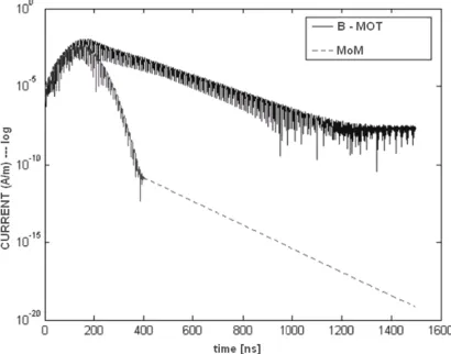
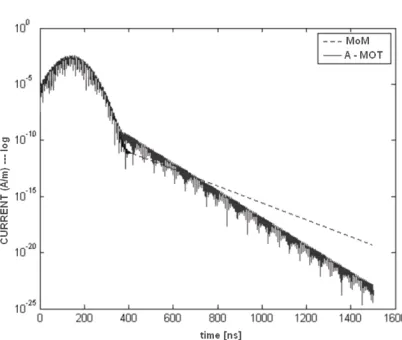
in Sections 5.1 and 5.2. Currents can be calculated by calculating the integrals included in Eq. (28) and Eq. (29) and adding them into Eq. (25). Comparison of the currents calculated by using the B-MOT and analytic formulations presented in this section (and henceforth referred to as A-MOT) with those calculated by employing the time domain method of moments (MOM) [2] has been given in Section 6. It is observed that the results obtained with A-MOT are stable and accurate.
5.1. Calculation of ψm,p Expression Anatically
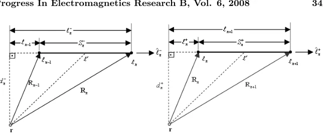
Integration ofhn(, t) can be written in terms of “+” and “−” egments as shown in Eq. (5) can be written as
hψn±(, t) =
Sn±
fn()
δ
t−R c
R d
=
n±1
n
n±1− s±n
ˆ
±n δ
t−R c
R d
= c n±1
n
n±1− s±n
ˆ
±nδ(ct
−R)
R d
(30)
At last step of Eq. (30), the rule which has been given below is used.
S δ
t−|r| c
dr=c
S
δ(ct− |r|)dr (31)
In Eq. (30),R has been defined as
R =
()2+d±n 2 (32)
As its known square root function has double value, socan be defined as
=χ
|r−r|2−d± n
2
; χ=
!
−1 ˆ·(r−r)<0
Figure 2. Definition of the basis function’s two segments.
Here, d±n, as shown in Figure 2, is perpendicular distance between observation point and the wire segment and it can be defined as
d±n = "
|R|2− |R·ˆ±|2 (34) By exchanging integration variable withR, d can be written as
d = RdR
χ
R2−d± n
2 (35)
By using Eq. (35), Eq. (30) can be written as
hψn±(, t) =cˆ±n Rn±1
Rn
n±1−χ
R2−d±n 2 s±n
δ(ct−R)
R
RdR χ
R2−d± n
2 (36) By using the rule given in Eq. (37)
S
δ(t−τ)f(τ)dτ =f(t) t∈S (37)
Eq. (36) can be written as
hψn±(, t) = ˆ±n
χn±1 s±n
1 $ % % &(t)2−
'
d±n c
(2 − c s±n
; Rn
c <
> t <> Rnc±1
By using Table 1, Eq. (38) can be defined as
hψn±(, t) = ˆn
" C1
(t)2−C2 2
−C3
; Rn
c < > t <>
Rn±1
c (39)
In Eq. (28),Vn(, tp−ti) expression defined as
Vψn(, tp−ti) = ∞
−∞
Ti(tp−t)hψn(, t)dt
= ∞
−∞
Ti(tp−t)hnψ+(, t)dt+
∞
−∞
Ti(tp−t)hψn−(, t)dt
(40)
In Eq. (40),Ti(tp−t) can be written asT(tp−ti−t) =T(tq−t) and according to [8] temporal basis funcitonT(tq−t) can be given as
T(tq−t) =
(tq−t)2
2∆t2 +
3(tq−t)
2∆t + 1 ; tq ≤t
≤tq+ ∆t
−(tq−t)2
∆t2 + 1 ; tq−∆t≤t≤tq (tq−t)2
2∆t2 −
3(tq−t)
2∆t + 1 ; tq−2∆t≤t
≤tq−∆t (41) or
T(tq−t) =e(t)2+f t+g (42) In Eq. (42),e, f and g denotes constant coefficients.
By substituting Eq. (39) and Eq. (42), Eq. (40) can be written as
Vψn(, tp−ti) = ˆn
Rn+1 c
Rn c
(e(t)2+f t+g) " C1
(t)2−C2 2
−C3
dt
+ˆn
Rn c
Rn−1 c
(e(t)2+f t+g) " C1
(t)2−C2 2
−C3
dt (43)
This integration can be calculated by using Table 2. Then, by calculating
Zmn,pψ −i=
Sm
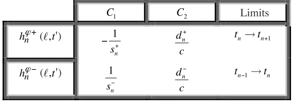
Table 1. Coefficients for Eq. (39).
1
C C2 C3 ˆn
n + h 1 1 n n n χ + + − n d c + 1 n n c + − ˆ n 1
nt →nt+
n − h 1 1 n n n χ − − − n d c − 1 n n c + − ˆ n
tn −1→tn
− + − Limits
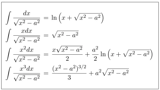
Table 2. Integration table.
dx √
x2−a2 = ln
x+*x2−a2
xdx
√
x2−a2 =
*
x2−a2
x2dx √
x2−a2 =
x√x2−a2
2 +
a2
2 ln
x+*x2−a2
x3dx √
x2−a2 =
(x2−a2)3/2
3 +a
2*x2−a2
Here, integration can be calculated numerically as in Section 3. The
ψm,p term can be written in the matrix form as ψm,p = µ
4π
n=1
i
In,iZmn,pψ −i (45)
5.2. Calculation of ϕm,p Expression Analytically
In Eq. (29),hϕn(, t) expression was given as
hϕn(, t) =
Sn
[∇ ·fn()]δ(t
−R/c)
R d
In Eq. (46), divergence term can be define as
∇ ·fn() = 1
s−n
∈Sn− − 1
s+n
∈Sn+
(47)
By using Eq. (47), Eq. (46) can be written as
hϕn±(, t) =
Sn−
1
s−n
δ(t−R/c)
R d
hϕn−(,t)
− Sn+
1
s+n
δ(t−R/c)
R d
hϕn+(,t)
(48)
By using the rule given in Eq. (50), Eq. (48) can be re-arranged as
hϕn±(, t) =c n
n−1
1
s−n
δ(ct−R)
R d
−c
n+1
n
1
s+n
δ(ct−R)
R d (49) S δ
t−|r| c
dr=c
S
δ(ct− |r|)dr (50)
By exchanging integration variable withR, Eq. (49) can be written as
hϕn±(, t) = c n
n−1
1
s−n
δ(ct−R)
R/
R/dR χ
R2−d±n 2
−c n+1
n
1
s+n
δ(ct−R)
R/
R/ dR χ
R2−d± n
2 (51)
By using the rule given in Eq. (37), Eq. (51) can be shown as
hϕn±(, t) =c 1 s−n
dR χ
ct−d±n 2−c
1
s+n
dR χ
ct−d±n
2; Rn <
> ct<> Rn±1
=∓c 1 s±n
dR χ
ct−d±n
2; Rn <
Table 3. Coeffients used inϕm,p integration.
1
C C2
,
n
hϕ + t' 1
n
s+
− dn
c +
1
n n
t →t +
n
hϕ− t 1
n s− n d c − 1 n n
t− →t
( ) , ' ( ) Limits
By using Table 3, Eq. (52) can be arranged as
hϕn±(, t) =C1
dR χ
(t)2−d±n 2
; Rn<> ct<> Rn±1 (53)
Vnϕ(, tp−ti) expression in Eq. (29) was given as
Vnϕ(, tp−ti) = ∞
−∞
Ti(tp−t)hnϕ±(, t)dt (54)
By substituting Eq. (42), Eq. (54) can be written as
Vnϕ(, tp−ti) =
Rn+1 c
Rn c
(e(t)2+f t+g) " C1
(t)2−C2 2 dt + Rn c
Rn−1 c
(e(t)2+f t+g)
C1
"
(t)2−C2 2
dt (55)
Vϕ
n(, tp−ti) can be found in a similar way which ψm,p was calculated
in Section 5.2 as
Vnϕ(, tp−ti) =C1
e t "
(t)2−C2 2 2 + C2 2 2 ln
t+ "
(t)2−C2 2 b a +f "
(t)2−C2 2 b a +g ln
t+ "
+C1 e t "
(t)2−C2 2
2 +
C22
2 ln
t+ "
(t)2−C2 2 b a
+f"(t)2−C2 2 b a +g ln
t+ "
(t)2−C2 2 b a (56)
In Eq. (29),Zmn,pϕ −i expression can be calculated as
Zmn,pϕ −i=c2
Sm
[∇ ·fm()]Vnϕ(, tp−ti)d (57)
Here, integration can be calculated numerically as in Section 3. ϕm,p
term in Eq. (29) can be written in the matrix form as
ϕm,p = µ 4π N n=1 i
In,iZmn,pϕ −i (58)
6. NUMERICAL RESULTS 6.1. A Small Dipole
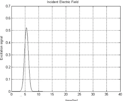
Usually, the Gaussian pulse is the most popular excitation used for the computation of transient responses of objects. It is wanted to be of finite duration in time and also band-limited in the frequency-domain. Gaussian plane waves which can be seen from Figure 4 can be defined mathematically as
Ei(r, t) = ˆpcos(2πf0τ) exp
−(τ −td)2
2σ2
(59)
wheref0 = 50 MHz is the center frequency,τ =t−r·k/cˆ is retarded time, ˆk = ˆx is the propagation direction, ˆp = ˆz is the polarization,
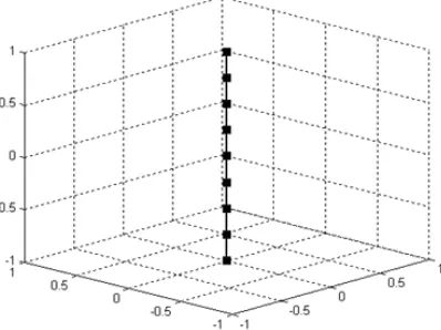
Figure 3. Straight thin wire structure.
Figure 4. Incident electric field.
Figure 5. Induced current in thin wire’s middle point (log).
Figure 6. Comparison of MoM solution and B-MOT solution for thin wire structure.
produced by employing the time domain moment method and as seen from the Figure 10, A-MOT formulation produces stable results even
Figure 7. Current distribution calculated by B-MOT on thin wire’s middle point (log) for the valuesβ = 0.15, b= 0.20 andβ = 0.25.
Figure 8. Comparison of the current calculated by using the B-MOT and the current calculated by using A-MOT for straight thin wire structures.
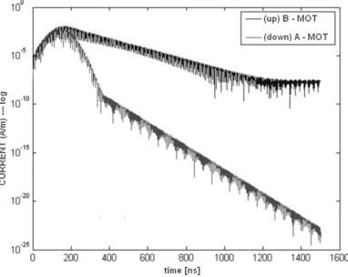
6.2. Loop Antenna
Gaussian pulse which can be seen from the Figure 11 is represented by
Ei(r, t) =E0 4
T√πe
−γ2 (60)
where γ = (4/T)(ct−cto−r·k), c is the velocity of light, k is the
Figure 9. Comparison of MoM solution and A-MOT solution for straight thin wire structure.
Figure 10. Current distribution calculated by A-MOT on thin wire’s middle point (log) for the values β = 1, β = 0.6, β = 0.25 and
β = 0.2.
pulse reaches its peakand choosen ascto= 6. Both of these quantities
Figure 11. Incident electric field.
Figure 12. Loop antenna.
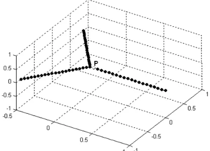
6.3. Three-Pole Structure
The modulated plane wave is used in [4] can be given as
Ei(r, t) = 4
T√πE0e
−γ2cos
2πf0
'
t−t0− r·kˆ
c
(
(61)
where
γ= 4c
T
'
t−t0− r·kˆ
c
(
Figure 13. Current distribution calculated by B-MOT for loop antenna on the point (0.5,0).
Figure 14. Three pole structure.
WithE0 linked to the maximum amplitude of the incident field, T is the time length of the impulse expressed in light metres (LM), t0 is the delay time of the incident pulse from the start of the simulation, ˆ
k is a unit vector, indicating the incidence direction of the wave, and
Figure 15. Current distribution on the point “P” for three pole structure calculated by B-MOT.
REFERENCES
1. Shanker, B., A. A. Ergin, K. Ayg¨un, and E. Michielssen, “Analysis of transient electromagnetic scattering from closed surfaces using a combined field integral equation,” IEEE Trans. Antennas Propagat., Vol. 48, No. 7, 1064–1074, 2000.
2. Ozsoy, S¨ ¸., “˙Ince tellerden olu¸san yapılardan sa¸cılma analizi ˙ı¸cin zamana ve frekansa ba˘glı˙ıki ¸c¨oz¨uc¨u,” Gebze Institute of Technology, 2003.
3. Ji, Z., T. K. Sarkar, B. H. Jung, Y. S. Chung, M. Salazar-Palma, and M. Yuan, “A stable solution of time domain electric field integral equation for thin-wire antennas using the Laguerre polynomials,” IEEE Trans. Antennas Propagat., Vol. 52, 2641– 2649, 2004.
4. Guarnieri, G., S. Selleri, G. Pelosi, C. Dedeban, and C. Pichot, “Innovative basis and weight functions for wire junctions in time domain moment method,”IEE Proc. - Microw. Antennas Propag., Vol. 153, 61–66, 2006.
5. Taflove, A., Computational Electrodynamics: The Finite-Difference Time-Domain Method, Artech House, Boston, MA, 1996.
the transient cattering by conducting surfaces of arbitrary shape,” IEEE Trans. Antennas Propagat., Vol. 40, 661–665, 1992.
8. Rynne, B. P. and P. D. Smith, “Stability of time marching algorithms for the electric field integral equation,”J. Electromagn. Waves Appl., Vol. 4, 1181–1205, Dec. 1990.
9. Sadigh, A. and E. Arvas, “Treating the instability in matching-on-in-time method from a different perspective,” IEEE Trans., Vol. AP-41, Dec. 1993.
10. Smith, P. D., “Instabilities in time marching methods for scattering: Cause and rectification,” Electromagn., Vol. 10, 439– 451, 1990.
11. Hu, J. L., Chi H. Chan, and Y. Xu, “A new temporal basis function for the time-domain integral equation method,” IEEE Microwave and Wireless Communications, Vol. 11, No. 11, Nov. 2001.
12. Wang, Y. and T. Itoh, “Envelope-Finite-Element (EVFE) tech-nique a more efficient time-domain scheme,” IEEE Transactions on Microwave Theory and Techniques, Vol. 49, 2241–2247, 2001. 13. Manara, G., A. Monorchio, and R. Reggiannini, “A space-time
discretization criterion for a stable time-marching solution of the electric field integral equation,”IEEE Trans. Antennas Propagat., Vol. 45, 527–532, 1997.