NEW TECHNIQUES TO CONQUER THE IMAGE RESOLUTION ENHANCEMENT PROBLEM S. E. El-Khamy
Department of Electrical Engineering Faculty of Engineering
Alexandria University Alexandria 21544, Egypt
M. M. Hadhoud
Department of Information Technology Faculty of Computers and Information Menoufia University
32511, Shebin Elkom, Egypt
M. I. Dessouky, B. M. Salam, and F. E. A. El-Samie Department of Electronics and Electrical Communications Faculty of Electronic Engineering
Menoufia University 32952, Menouf, Egypt
1. INTRODUCTION
In most electronic imaging applications, images with high resolution (HR) are required. HR means that pixel density per unit area in the image is high, and therefore an HR image can offer more details, which are of great importance in many applications. For example, HR images are very helpful in medical applications to facilitate the diagnosis process. HR images are also required in applications such as military imaging because images are captured at remote distances. Satellite space imagery is one of the fields that have a bad need for obtaining HR images from the available captured LR images. In applications such as image compression, LR images are transmitted to save the bandwidth and therefore it is the task of the receiver to obtain HR images from the received LR images. In the processing of old movies, it’s also required to obtain HR multi frames from the available LR multi frames. All these applications have motivated the emergence of a new field of image processing called HR image processing.
In recent years, digital imaging cameras for both still images and movies have been widely developed. These cameras are based on charge-coupled devices (CCDs) and CMOS image sensors. Although these imaging cameras have so many advantages compared to classical cameras used previously, they suffer from the problem of limited spatial resolution and their resolution levels and consumer prices are not suitable for future applications. Thus, the limited abilities of digital cameras has been another motivation for the emergence of the HR image processing branch.
The branch of HR image processing concentrates on two main topics, image interpolation and image super resolution. Image interpolation is the process by which a single HR image can be obtained from a single degraded LR one [1–17], while super-resolution reconstruction of images aims at obtaining a single HR image either from several degraded still images or from several degraded multiframes [18–33]. This paper introduces a group of image interpolation and image super-resolution algorithms and some comparisons between them.
2. SINGLE CHANNEL LR IMAGE DEGRADATION MODEL
In the imaging process, when a scene is imaged by an HR imaging device, the captured HR image can be namedf(n1, n2) wheren1, n2 =
0,1,2, . . . , M −1. Here M =N/R, where R is the ratio between the sampling rates of f(n1, n2) and g(m1, m2). The relationship between
the LR image and the HR image, assuming no blurring, can be represented by the following mathematical model [9–12]:
g=Df+v (1)
wheref,gandv are lexicographically ordered vectors of the unknown HR image, the measured LR image and additive noise values, respectively. The f vector is of size N2 ×1 and the vectors g and
v are of sizeM2×1. The matrixD is of sizeM2×N2. The matrixD
represents the filtering and down sampling process, which transforms the HR image to the LR image. Under separability assumption, the model of filtering and down sampling processes which transforms the
N ×N HR image to theM ×M LR image is shown in Fig. 1. Here
M =N/2.
Horizontal
LPF ↓2
Vertical
LPF ↓2
f(n1,n2) HR image
g(m1,m2)
LR image
Figure1. Down sampling process from the N ×N HR image to the
N/2×N/2 LR image.
3. IMAGE INTERPOLATION
The process of image interpolation aims at estimating intermediate pixels between the known pixel values in the available LR image. The image interpolation process can be considered as an image synthesis operation. This process is performed on a one dimensional basis; row by row and then column by column. If we have a discrete sequence
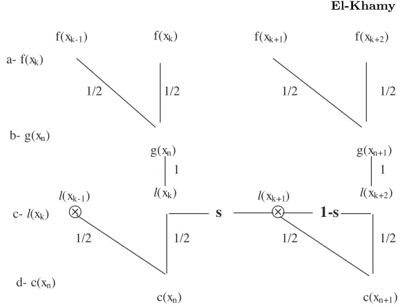
f(xk) of length N as shown in Fig. 2a and this sequence is filtered
and down sampled by 2, we get another sequenceg(xn) of lengthN/2
as shown in Fig. 2b. The interpolation process aims at estimating a sequence l(xk) of length N as shown in Fig. 2c, which is as close as
possible to the original discrete sequence f(xk).
3.1. Linear SpaceInvariant ImageInterpolation
For equally spaced 1-D sampled data, g(xn), many interpolation
functions can be used. The value of the sample to be estimated,
l(xk+1), can, in general, be written in the form [1–12]:
l(xk+1) =
∞
n=−∞
a- f(xk)
g(xn+1)
g(xn)
b- g(xn)
l(xk+2)
c- l(xk)
c(xn+1)
c(xn)
d- c(xn)
1/2 1/2
1/2
1 1
1/2 1/2
1/2 1/2
1/2
l(xk-1) l(xk) l(xk+1)
⊗
s⊗
1-sf(xk-1) f(xk) f(xk+1) f(xk+2)
Figure2. Signal down sampling and interpolation. a- Original data sequence.
b- Down sampled version of the original data sequence. c- Interpolated data sequence.
d- Down sampled version of the interpolated data sequence.
whereβ(x) is the interpolation basis function.
From the classical Sampling theory, if g(xn) is band limited to
(−π, π), then [1–12]:
l(xk+1) =
∞
n=−∞
g(xn)sinc (xk+1−xn) (3)
This is known as ideal interpolation. From the numerical computations point of view, the ideal interpolation formula is not practical due to the slow rate of decay of the interpolation kernel sinc (x). So, approximations such as nearest-neighbor, bilinear, B-Spline, Key’s (bicubic) and o-Moms basis functions are used as alternative basis functions [1–12].
Thus, Eq. (2) can be implemented on a finite neighborhood rather than carrying out an infinite summation and the coefficientscnneed to
be estimated [1–12]. The choice of the basis functionβ(x) can save the step of estimating the coefficientscnif it is chosen to be an interpolating
3.1.1. Nearest-Neighbor Interpolation
Nearest-neighbor interpolation is the simplest interpolation scheme. The basis function associated with nearest-neighbor interpolation is given by [1–12]:
β0(x) =
0 x <−1/2 1 −1/2≤x≤1/2 0 1/2≤x
(4)
This scheme of interpolation is merely a pixel repetition process and the basis function is interpolating.
3.1.2. Bilinear Interpolation
The bilinear interpolation enjoys a large popularity due to its simplicity of implementation. The basis function used in bilinear interpolation is interpolating and it’s given by [1–12]:
β1(x) =
1− |x| |x|<1
0 1≤ |x| (5)
As shown in Fig. 2, we define the distance between xk+1 and xn and
betweenxk+1 and xn+1 as [13–17]:
s=xk+1−xn, 1−s=xn+1−xk+1 (6)
Thus, Eq. (2) can be written as follows [1–12]:
l(xk+1) = (1−s)g(xn) +sg(xn+1) (7)
3.1.3. B-Spline Interpolation
There is a whole family of interpolation basis functions called B-Splines. These functions are piecewise polynomials of degree n. T he basis functionβn(x) represents the central B-Spline of degreenwhich is given by [1–12]:
βn(x) =β0∗β0∗ · · · ∗β0(x)
(n+1) times
(8)
the cubic spline basis function is given by [1–12]:
β3(x) =
2 3− |x|
2+|x|3
2 0≤ |x|<1 (2− |x|)3
6 1≤ |x|<2
0 2≤ |x|
(9)
The cubic spline interpolation formula is given by:
l(xk+1) = c(xn−1)[(3 +s)3−4(2 +s)3+ 6(1 +s)3−4s3]/6
+c(xn)[(2 +s)3−4(1 +s)3+ 6s3]/6
+c(xn+1)[(1 +s)3−4s3]/6 +c(xn+2)s3/6 (10)
B-spline basis functions are non-interpolating and thus, the coefficients in Eq. (2) need to be estimated prior to the interpolation process. This estimation process can be implemented using a digital filtering approach [1–12].
3.1.4. Bicubic Interpolation
Another method which is significantly effective in signal interpolation is the bicubic one. The bicubic interpolation basis function is interpolating and can be expressed in the following form [8, 11]:
β(x) =
(α+ 2)|x|3−(α+ 3)|x|2+ 1 0≤ |x| ≤1
α|x|3−5α|x|2+ 8α|x| −4α 1<|x| ≤2 (11) Thus, the general bicubic interpolation formula is given by [8, 11]:
l(xk+1) =g(xn−1)[αs3−2αs2+αs] +g(xn)[(α+ 2)s3−(3+α)s2+ 1]
+g(xn+1)[−(α+2)s3+(2α+3)s2−αs]+g(xn+2)[−αs3+αs2]
(12)
whereα is an optimization parameter. It may be adaptive from point to point depending on the signal local activity levels.
3.1.5. O-Moms Interpolation
as the weighted sum of a B-Spline and its derivatives [5, 6]. For cubic o-Moms image interpolation , the basis function is given by [5, 6]:
o−M oms3(x) =
1 2|x|
3− |x|2+ 1
14|x|+ 13
21, 0≤ |x| ≤1 −1
6 |x|
3+|x|2+ 85
42|x|+ 29
21, 1<|x| ≤2
0, 2≤ |x|
(13)
The o-Moms basis functions are non-interpolating and thus the coefficients in Eq. (2) need to be estimated. This estimation process can be implemented using the same digital filtering approach as in B-Spline image interpolation [5, 6].
3.2. AdaptiveImageInterpolation (TheWarped Distance Approach)
The idea of warped distance can be used in any of the techniques mentioned in Section 2 to improve their performance. This idea is based on modifying the distance s and using a new distance s based on the homogeneity or inhomogeneity in the neighborhood of each estimated pixel. The warped distance s can be estimated using the following relation [9]:
s=s−τ Ans(s−1) (14)
whereAn refers to the asymmetry of the data in the neighborhood of x and it is defined as [9]:
An= |
g(xn+1)−g(xn−1)| − |g(xn+2)−g(xn)|
L−1 (15)
where L= 256 for 8 bit pixels. The scaling factor L is to keep An in
the range of−1 to 1.
The parameterτ controls the intensity of warping to avoid blurring of edges in the interpolation process.
3.3. AdaptiveImageInterpolation Based on Local Activity Levels
AdaptiveBilinear
l(xk+1) =a0(1−s)g(xn) +a1sg(xn+1) (16)
where,
a0 = 1−λAn, a1 = 1 +λAn (17)
AdaptiveBicubic
l(xk+1) = a−1g(xn−1)[αs3−2αs2+αs]
+a0g(xn)[(α+ 2)s3−(3 +α)s2+ 1]
+a1g(xn+1)[−(α+ 2)s3+ (2α+ 3)s2−αs]
+a2g(xn+2)[−αs3+αs2] (18)
AdaptiveCubic Spline
l(xk+1) = a−1c(xn−1)[(3 +s)3−4(2 +s)3+ 6(1 +s)3−4s3]/6
+a0c(xn)[(2 +s)3−4(1 +s)3+ 6s3]/6
+a1c(xn+1)[(1 +s)3−4s3]/6 +a2c(xn+2)s3/6 (19)
where in (18) and (19),
a−1=a0 = 1−λAn, a1 =a2= 1 +λAn (20)
and λis a constant which controls the intensity of weighting used for neighboring pixels. Thus, the weighting coefficients are updated at each pixel depending on the asymmetryAn at this pixel. We note the
following special cases:
i- For homogeneous regions, the value of An tends to zero which
leads to a−1 = a0 = a1 = a2 = 1. This is equivalent to the
traditional image interpolation process.
ii- For positive values ofAn, which means that there is an edge that
is more homogeneous on the right side, the weights of the pixels on the right side (a1 and a2) are increased and the weights of the
pixels on the left side (a−1 anda0) are decreased. This is expected
to yield images with better visual quality.
iii- For negative values ofAn,a−1 anda0 are increased anda1and a2
are decreased and the same effect is obtained.
(a) Original Mandrill image (b) LR Mandrill image.
(c) Bicubic Interpolation (no warping). MSE=826.7
(d) Bicubic interpolation with warping . MSE=807.4
(e) Adaptive Image Interpolation (no warping) MSE=791
(f) Adaptive image interpolation with warping. MSE=786.4
(a) Squared error for bicubic image interpolation
(b) Squared error for adaptive bicubic image interpolation
Figure4. Squared error at each pixel for the interpolated Mandrill image.
Table1. MSE for interpolation of the LR Mandrill image using the simple adaptive algorithm.
Interpolation
with no
warping
Warped distance Interpolation
Adaptive Weighted interpolation
Adaptive weighted Interpolation with warping
Bilinear 845.09 830.72 808.26 805.72
Bicubic 826.7 807.4 791 786.4
Cubic -spline 855.5 846.23 819.96 816.84
3.4. SpaceVarying PBP ImageInterpolation
Equations (7) and (10) have a single controlling parameter s while Eq. (12) has two controlling parameterssandαwhich can be optimized to give the best interpolation results. The adaptation can be made pixel by pixel (PBP) depending on the neighboring pixel values [17]. Suppose we have a discrete sequence f(xk) of length N as illustrated
in Fig. 2a. Applying the process of filtering and down sampling on this sequence, we get a sequence g(xk) of length N/2 as given in
Fig. 2b. If we apply a polynomial based interpolation process on the resulting sequence g(xn), we will get a sequence l(xk) of length N
minimization of the mean squared error (MSE) between the estimated sequence and the original sequence. The minimization of the MSE can be performed by the minimization of the squared error between each estimated sample and its original value.
If the sequenceg(xn) is interpolated using bilinear interpolation to
givel(xk), the squared estimation error between the estimated sample l(xk+1) and the original samplef(xk+1) is given by [11, 12]:
E= [f(xk+1)−l(xk+1)]2 (21)
Substituting for l(xk+1) from Eq. (7), we get:
E = [f(xk+1)−(1−s)g(xn)−sg(xk+1)]2 (22)
But from Fig. 2, we have the following relations:
g(xn) =
1
2[f(xk) +f(xk−1)] (23)
g(xn+1) =
1
2[f(xk+2) +f(xk+1)] (24) Substituting for g(xn) and g(xn+1) into Eq. (21), we get [12]:
E=
f(xk+1)−
(1−s)
2 [f(xk) +f(xk−1)]−
s
2f(xk+2) +f(xk+1)]
2
(25) All sample values are considered constants and E is a function of s
only.
Differentiating Eq. (25) with respect to s and equating to zero gives [12]:
sopt =
f(xk+1)−g(xn) g(xn+1)−g(xn)
(26)
Thus, atsopt, there is a minimum squared error between the estimated
sample l(xk+1) and the original sample f(xk+1) [12]. The same
treatment is possible for all other interpolation methods [12].
It is noted that the sequence g(xn) is available but the sequence f(xk) is unavailable. Thus, one cannot directly determinesopt for the
above mentioned four cases. To solve this problem, we apply a down sampling operation on the sequence l(xk) to get a sequence q(xn) of
length N/2 as illustrated in Fig. 2d. The squared estimation error betweenq(xn+1) and g(xn+1) is given by:
From Fig. 2, we have:
l(xk+2) =g(xn+1) (28)
and
q(xn+1) =
1
2[l(xk+1) +l(xk+2)] (29) Substituting from Eqs. (24), (28) and (29) into Eq. (27), we get:
E∗ = 1 4
[f(xk+1)−l(xk+1)] +
1
2[f(xk+2)−f(xk+1)]
2
(30)
Substituting from Eq. (21) into Eq. (30), we get [12]:
E∗ = 1 4
√
E+K2 (31)
where
K = 1
2[f(xk+2)−f(xk+1)] (32) It is clear thatK is a constant with respect to s or with respect to s
and α for the bicubic case. For the case of edge interpolation, which is the case of our greatest interest, the side containing f(xk+1) and f(xk+2) is homogeneous and the side containingf(xk−1) andf(xk) is
also homogeneous. This means that the values off(xk+1) and f(xk+2)
are close to each other and the values of f(xk−1) and f(xk) are also
close to each other. Thus, the value of K is small and therefore, the value of sopt which minimizes E leads to the minimization of E∗
regardless of the sign of K. SinceE is minimum atsopt, then E∗ will
be minimum at the same value of sopt. For flat areas, the constantK
is approximately equal to zero and E∗∼=E/4.
From Eq. (31), we can deduce the following equation [11, 12]:
Emin∗ = 1 4
Emin+K 2
(33)
To evaluate the value of sopt for the cases of bilinear and cubic Spline
interpolation, we follow an iterative manner as follows [12]:
si+1 =si−η0 dE∗
ds (si) (34)
whereη0 is the convergence parameter ands0= 1/2.
From Eq. (27), we get:
dE∗
ds =−2[g(xn+1)−q(xn+1)]
dq(xn+1)
ds (35)
Substituting from Eq. (29) into Eq. (35), we get:
dE∗
ds =−
g(xn+1)−
1
2[l(xk+1) +l(xk+2)]
dl(xk+1)
ds (36)
The termdl(xk+1)
ds is calculated for each interpolation formula as follows:
i- Bilinear[12]:
dl(xk+1)
ds =−g(xn) +g(xn+1) (37)
ii- Cubic spline[12]:
dl(xk+1)
ds = c(xn−1)[3(3 +s)
2−12(2 +s)2+ 18(1 +s)2−12s2]/6
+c(xn)[3(2 +s)2−12(1 +s)2+ 18s2]/6
+c(xn+1)[3(1 +s)2−12s2]/6 +c(xn+2)s2/2 (38)
For the case of bicubic interpolation, we have two controlling parameters s and α. If the sequence g(xn) is interpolated using
the bicubic interpolation formula, then using Eq. (21), the squared estimation error between l(xk+1) and the original sample f(xk+1) is
given by [11]:
E = [f(xk+1)−l(xk+1)]2
= [f(xk+1)−g(xn−1)[αs3−2αs2+αs]
−g(xn)[(α+ 2)s3−(3 +α)s2+ 1]
−g(xn+1)[−(α+2)s3+(2α+3)s2−αs]−g(xn+2)[−αs3+αs2]]2
(39)
It is required to find the values ofsoptandαoptthat minimize the value
of E in Eq. (39).
The error functionE∗ is a function of the two parameters s and
α. Thus, the minimization of E∗ can be performed by equating the gradient of E∗ to zero [11].
∇E∗(s, α) =
∂E∗(s, α)
∂s ∂E∗(s, α)
∂α
The values ofsopt andαopt can be iteratively estimated as follows [11]:
si+1 αi+1
= si αi
−η0∇E∗(si, αi) (41)
whereη0 is the convergence parameter ands0= 1/2 andα0 =−1/2.
If α is fixed at −1/2 and the optimization is carried out with respect tosonly, Eq. (41) is simplified to the form [11]:
si+1 =si−η0 dE∗
ds (si) (42)
Ifsis fixed at 1/2 and the optimization is carried out with respect to
α only, Eq. (41) is simplified to the form [11]:
αi+1 =αi−η0 dE∗
dα (αi) (43)
The values of ∂E∂s∗ and ∂E∂α∗ are calculated from Eq. (27) as follows [11]:
∂E∗
∂s = −2[g(xn+1)−q(xn+1)]
∂q(xn+1)
∂s (44)
∂E∗
∂α = −2[g(xn+1)−q(xn+1)]
∂q(xn+1)
∂α (45)
Substituting from Eqs. (18) and (28) into Eq. (29), we get [11]:
q(xn+1) =
1
2g(xn−1)[αs
3−2αs2+αs]+1
2g(xn)[(α+2)s
3−(3+α)s2+1]
+1
2g(xn+1)[−(α+ 2)
3+ (2α+ 3)s2−αs+ 1] + 1
2g(xn+2)[−αs
3+αs2]
(46)
Using Eq. (46), we get [11]:
∂q(xn+1)
∂s =
1
2g(xn−1)[3αs
3−4αs+α]+1
2g(xn)[3(α+2)s
3−2(3+α)s]
+1
2g(xn+1)[−3(α+ 2)s
2+ 2(2α+ 3)s−α] + 1
2g(xn+2)[−3αs
2+ 2αs]
(47)
∂q(xn+1)
∂α =
1
2g(xn−1)[s
3−2s2+s]+1
2g(xn)[s
3−s2]
+1
2g(xn+1)[−s
3+ 2s2−s] + 1
2g(xn+2)[−s
3+s2]
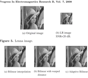
(a) Original image (b) LR image SNR=20 dB.
Figure5. Lenna image.
(a) Bilinear interpolation (b) Bilinear with warped distance
(c) Adaptive Bilinear
Figure6. Bilinear interpolation (SN R= 20 dB).
This iterative algorithm is used for the estimation of each pixel in the interpolation process. The optimization process of the bicubic image interpolation formula can be performed either with respect to a single parameter (s orα) or with respect to both parameters.
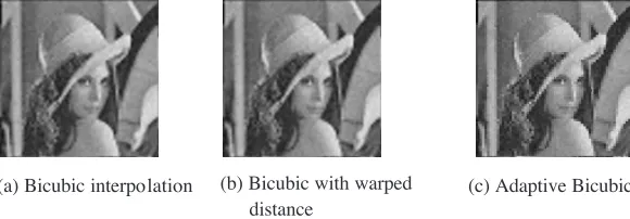
Several experiments have been carried out to test the suggested adaptive image interpolation algorithm on the Lenna image given in Fig. 5. The results given in Figs. 6 to 9 reveal that the suggested adaptive image interpolation algorithm is better in performance than the traditional algorithms.
Other experiments on the above mentioned algorithms with different images have also been carried out and the results are given in Tables 2 to 4. These results show that the suggested adaptive algorithm gives better results for different images with different signal to noise ratios.
3.5. InverseImageInterpolation
(a) Cubic Spline (b) Cubic Spline with warped distance (c) Adaptive Cubic Spline
Figure7. Cubic Spline interpolation (SN R= 20 dB).
(a) Bicubic interpolation (b) Bicubic with warped distance
(c) Adaptive Bicubic
Figure8. Bicubic interpolation (SN R= 20 dB).
10 20 30 40
200 300 400 500
SNR(dB)
MSE
(a)
bilinear warped dist. adaptive
10 2 0 30 40 200
300 400 500
SNR(dB)
MSE
(b)
bicubic warped dist. adaptive
10 20 30 40
200 300 400 500
SNR(dB)
MSE
(c)
cubic spline warped dist. adaptive
Table2. MSE for bilinear interpolation of different images. Bilinear Bilinear
(warped distance)
Adaptive Bilinear
Bilinear Bilinear (warped distance)
Adaptive Bilinear Image
Noise Free interpolation SNR=20 dB
Cameraman 253 237 197 274 257 234
Lenna 336 333 269 347 346 289
Mandrill 834 800 685 852 820 716
Building 1201 1170 965 1213 1183 983
TestPat1 333 345 277 359 370 324
Table3. MSE for bicubic interpolation of different images. Bicubic Bicubic
(warped distance)
Adaptive Bicubic
Bicubic Bicubic (warped distance)
Adaptive Bicubic Image
Noise Free interpolation SNR=20 dB
Cameraman 243 223 194 267 249 231
Lenna 327 324 270 341 339 289
Mandrill 818 772 690 840 798 722
Building 1207 1164 966 1223 1176 979
TestPat1 304 319 263 335 348 308
Table4. MSE for cubic spline interpolation of different images.
Cubic Spline Cubic Spline (warped distance) Adaptive Cubic Spline Cubic Spline Cubic Spline (warped distance) Adaptive Cubic Spline Image
Noise Free interpolation SNR=20 dB
Cameraman 251 215 215 281 255 255
Lenna 329 314 273 330 347 295
Mandrill 842 814 731 870 840 762 Building 1267 1240 1074 1281 1258 1090 TestPat1 298 267 267 334 310 310
3.5.1. Linear Minimum Mean Square Error (LMMSE) Image Interpolation
The LMMSE criterion requires the MSE of estimation to be minimum over the entire ensemble of all possible estimates of the image. The optimization problem here is given by [15, 17]:
min
ˆ
f
E[ete] =E[T r(eet)] (49)
with
e=f −fˆ (50)
where ˆf is the estimate of the HR imagef, which is captured assuming that an HR camera is used. Solving this optimization problem based on Eq. (1) leads to the following solution [15, 17]:
ˆ
f =RfDt(DRfDt+Rv)−1g (51)
In this solution, the noise is assumed to be independent on the image such that:
E[f vt] =E[vtf] = [0] (52)
The autocorrelation matrices given in Eq. (51) are defined as follows [15, 17]:
Rf =E[f ft] (53)
and
Rv =E[vvt] (54)
The matrixRv is a diagonal matrix whose main diagonal elements are
equal to the noise variance of the noisy LR image.
The matrixRf can be approximated by a block diagonal matrix
in the form [15, 17]:
Rf =
R00 0 · · · 0
0 R11 . .. ...
..
. . .. ... 0
0 · · · 0 RN−1N−1
(55)
If the samples of each column are assumed uncorrelated except for each pixel with itself, each matrix Rii can be approximated by a diagonal
matrix fori= 0,1, . . . , N−1.
The main diagonal elements of the matrix Rii can be
For an imagef(n1, n2), the autocorrelation at the spatial location
(n1, n2) can be estimated from the following relation [15, 17]:
Rf(n1, n2)∼=
1
w2 w
k=1 w
l=1
f(k, l)f(n1+k, n2+l) (56)
where w is an arbitrary window length for the autocorrelation estimation.
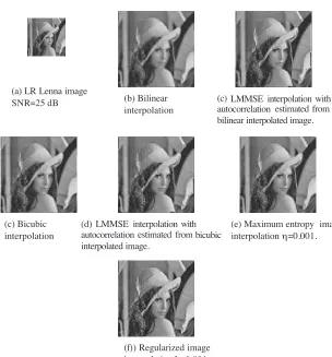
The imagef(n1, n2) may be taken as the bilinear, bicubic or cubic
spline interpolated image. Thus, the matrixRf can be approximated
by a diagonal sparse matrix.
3.5.2. Maximum Entropy Image Interpolation
If the samples of the lexicographically ordered image are normalized to a maximum of 1, these samples can be considered as probabilities. Thus, the entropy of the sampled image is defined as follows [17]:
E =−
N2
i=1
filog2(fi) (57)
whereE is the entropy andfi is the sampled signal.
This equation can be written in the vector form as follows [17]:
E =−ftlog2(f) (58)
For image interpolation, to maximize the entropy subject to the constraint that g−Df2 = v2, the following cost function must be minimized:
Ψ(f) =ftlog2(f)−λ
g−Df2− v2
(59)
whereλis a Lagrangian multiplier. Solving for ˆf leads to [17]:
ˆ
f ∼= (D∗tD+ηI)−1D∗tg (60) whereη=−1/(2λln(2)).
The inversion of the term D∗tD +ηI can be performed easily depending of the special nature of this matrix, which is a sparse matrix. The effect of the termηI is to remove the ill posedness nature of the inverse problem by redistributing the eigen values of the term D∗tD
3.5.3. Regularized Image Interpolation
Regularization theory was first introduced by Tikhonov and Miller. It provides a formal basis for the development of regularized solutions of ill posed problems [34–36]. The stabilizing function technique is one of the basic methodologies for the development of regularized solutions. According to this approach, an ill-posed problem can be regarded as the constrained minimization of a certain function, called the stabilizing function. The specific constraints imposed by the stabilizing function technique on the solution depend on the form and the properties of the stabilizing function used.
According to the regularization approach, the solution of Eq. (1) is obtained by the minimization of the following cost function [16, 17]:
Ψ(f) =g−Df2+λCf2 (61) where C is the regularization operator and λ is the regularization parameter.
This minimization is accomplished by taking the derivative of the cost function yielding:
∂Ψ(f)
∂f =0= 2D
t(g−Dfˆ)−2λCtCfˆ (62)
Solving for ˆf that provides the minimum of the cost function yields [16, 17]:
ˆ
f = (DtD+λCtC)−1Dtg (63) The solution of the regularized image interpolation problem can’t be solved as a direct inversion process for the whole image due to the large computational complexity of the inversion process. One of the possible previously suggested solutions to this problem is to use successive approximation techniques for the solution.
In this section, we suggest another solution to the regularized image interpolation problem. This solution is implemented by the segmentation of the LR image into overlapping segments and interpolating each segment alone using Eq. (63) [16, 17]. It is clear that, if a global regularization parameter is used, a single matrix inversion process for a matrix of small dimensions is required because the term (DtD +λCtC)−1 is independent on the image to be interpolated.
Thus, the algorithm is efficient from the point of view of computation time.
(a) LR Lenna image
SNR=25 dB (b) Bilinear interpolation
(c) Bicubic interpolation
(c)
autocorrelation
bilinear interpolated image.
(d) LMMSE interpolationwith autocorrelation
interpolated image.
(e) Maximum entropy image interpolation η=0.001.
(f)) Regularized image interpolation λ=0.001.
estimated from LMMSE interpolation with
estimated from bicubic
Figure10. Inverse interpolation results.
4. SUPER-RESOLUTION RECONSTRUCTION OF IMAGES
Table5. MSE Interpolation results for different images with SNR = 25 dB. Column 3 of LMMSE interpolation uses the bilinear interpolation in estimating the HR image autocorrelation matrix. Column 5 of LMMSE interpolation uses the bicubic interpolation in estimating the HR image autocorrelation matrix.
Image
Bilinear Interpolation
LMMSE Interpolation
Bicubic Interpolation
LMMSE Interpolation
Maximum Entropy Interpolation
η=0.001
Regularized Interpolation
λ=0.001
Cameraman 256 215 248 224 199 151
Lenna 341 284 332 290 280 219
Mandrill 259 215 255 216 218 202
Building 1156 862 1167 869 840 958
TestPat1 342 235 313 242 296 6 9
[20–24]. The special nature of this problem forces most image super resolution reconstruction algorithms to have an iterative nature. These algorithms aim at reducing the computational cost of the matrix inversion processes involved in the solution by using successive approximation methods for the estimation of the HR image.
Most of the previously suggested solutions to this problem are based on the regularization theory [18–29]. The iterative implementation of the regularization theory in image super resolution has been the most popular procedure to solve the problem. Although these algorithms avoid matrix inversions, they are still time consuming and can’t be implemented beyond a certain limit of dimensionality.
4.1. Multi-Channel LR Degradation Model
In super resolution image reconstruction algorithms, several degraded LR observations are used to estimate a single HR image. The mathematical model which relates the available LR observations to the required HR image is given by [18–33]:
gk=DkBkMkfh+vk 1≤k≤P (64)
where P is the number of available observations, gk is an (M2×1)
vector representing thekth (M×M) LR image in lexicographic order.
fh is an (N2 ×1) vector representing an (N ×N) HR image in lexicographic order. Mk is the (N2 ×N2) registration shift matrix
and Bk is the blur matrix of size (N2×N2). Dk is the (M2×N2)
uniform down sampling matrix. vk is the M2×1 noise vector.
Equation (64) can be rewritten in the following form:
g1 .. . gP =
D1B1M1
.. .
DpBpMp fh+
v1 .. . vP (65)
Simplifying Eq. (65) leads to:
g=Lfh+v (66)
where: g= g1 .. . gP
, L=
D1B1M1
.. .
DpBpMp
, v=
v1 .. . vP (67)
Using the regularization theory to solve Eq. (66), we get [76, 78, 83]:
ˆ
fh= [LtL+τCtC]−1Ltg (68)
where C is the regularization operator which is preferred to be the 3-D Laplacian operator to capture the between channel information in the reconstruction process. The parameterτ is a global regularization parameter.
4.2. Suggested Super Resolution Reconstruction Approach In this section, we suggest a new approach to image super resolution based on wavelet fusion [30–33]. The implementation of this approach is composed of four consecutive steps. In the general solution of the super resolution reconstruction problem, we deal with three degradation phenomena, a general geometric registration warp, blurring and additive noise. Based on these phenomena, we can break the solution into the following consecutive steps.
Step 1: Image alignment, which means estimating the geometrical registration warp between different images.
Step 2: Multi-channel image restoration of the registered degraded observations.
Step 3: Wavelet based fusion of the multiple images obtained from step 2 to form a single image.
Step 4: Image interpolation of the resulting image from step 3 to obtain an HR image.
4.3. Simplified Multi-Channel Degradation Model
The multi channel image restoration step aims at obtaining multiple undegraded images of the same dimensions as that of the available LR images. These obtained images are then used in the next step of image fusion. This step requires that a simplified degradation model is used. This model doesn’t consider the operator D of filtering and down sampling. For a multi channel imaging system withP channels each of sizeM×M, the simplified degradation model becomes [30–32]:
gk=BkMkfk+vk fork= 1,2, , . . . , P (69)
where gk,fk and vk are the observed image, the ideal image and the
noise of the kth channel, respectively. Bk is the degradation matrix
of the kth channel. Mk is the relative registration shift operator
of the kth channel. In this paper, we restrict our work to global translational shifts, which is the case of consideration in most image super resolution reconstruction algorithms. Translational motion can be approximated by circular motion except near edge pixels [30–32]. Using this approximation, the matrices Mk can be approximated by
circulant matrices for all values ofk.
Equation (69) can be written in the following form:
where g= g1 g2 .. . gP ; f =
f1 f2 .. . fP ; v =
v1 v2 .. . vP ; B =
B1 0 · · · 0
0 B2 · · · 0
..
. ... · · · ... 0 0 · · · BP
and M =
M1 0 · · · 0
0 M2 · · · 0
..
. ... · · · ... 0 0 · · · MP
(71)
If we define:
H =BM (72)
Then, the multi-channel image degradation model can be written in the form [30–32]:
g=Hf+v (73)
whereg,f andv areP×M2in length. The degradation operatorHof the multi channel-imaging model is of dimensions (P×M2)×(P×M2). We can assume f1=f2=· · ·=fP.
According to the model given in Eq. (73), the multi-channel rstoration process is similar to that of the inverse image interpolation process but withDreplaced byH. Thus, the same techniques used for inverse image interpolation are applicable for multi-channel restoration but with different implementation methods [30–34].
4.4. Multi Channel Image Restoration
4.4.1. Multi-Channel LMMSE Restoration
The LMMSE solution to the multi-channel image restoration problem is, thus, given by [30]:
ˆ
f =RfHt[HRfHt+Rv]−1g (74)
4.4.2. Multi-Channel Maximum Entropy Restoration
Using the concept of entropy maximization, the solution of the simplified multi-channel image degradation model is represented as follows [31]:
ˆ
4.4.3. Multi-Channel Regularized Restoration
Solving for ˆf using the regularization concept gives [32]:
ˆ
f = [HtH+Λ−1CtC]−1Htg (76)
whereΛ is defined by:
Λ=
λ1[I] 0 · · · 0 0 λ2[I] · · · 0
..
. ... · · · ...
0 0 · · · λP[I]
(77)
The identity matrixI is of sizeM2×M2.
The suggested super resolution image reconstruction algorithms are tested on different noisy LR degraded observations with different signal to noise ratios. Several experiments have been conducted in
this test. In the first experiment, three LR degraded observations
of Lenna image of size 128× 128 are used to obtain a single HR
image of size 256 × 256. The general degradation model of Eq.
(64) is used to generate the degraded observations. The degradation in each observation comprises a relative translational shift with the reference observation, an out of focus blurring and additive noise with
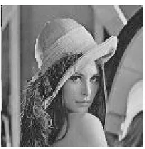
SN R = 40 dB. The original LR image is shown in Fig. 11. The
degraded observations are given in Fig. 12.
Figure 11. Original Lenna image.
(a) observation (1) 5×5 Blur operator
(b) observation (2) 7×7 Blur operator
(c) observation (3) 9×9 Blur operator
Figure 12. Available observationsSN R= 40 dB.
Figure 13. LMMSE interpolation of the original image.
(a)Fused Image PSNR=24.3 dB
(b)LMMSE interpolation of the fused image PSNR=24.2 dB
Figure 14. Results of the LMMSE Super-resolution reconstruction
Figure 15. Maximum entropy interpolation of the original image.
(a)Fused Image PSNR=26.43 dB
(b)Obtained HR image PSNR=26.47 dB CPU=10 sec on a 1 GHz Processor
Figure 16. Results of the maximum entropy super resolution
reconstruction algorithm.
The maximum entropy interpolated version of the original LR image is given in Fig. 15. The image obtained from the fusion of the outputs of multi-channel maximum entropy restoration step is given in Fig. 16a. The HR image obtained using the maximum entropy super
resolution algorithm is given in Fig. 16b. The parameterη used in the
multi channel restoration step and in the interpolation step is 0.001. It is clear from the obtained results that the computation time is reduced significantly and the visual quality and the PSNR value obtained get better.
Figure 17. Regularized interpolation of the original image.
(a) Fused Image PSNR=27.7 dB
(b)Obtained HR image PSNR=27.7 dB CPU=105 sec on a 1 GHz Processor
Figure 18. Results of the regularized super-resolution reconstruction
algorithm.
of multi-channel regularized restoration step is given in Fig. 18a. The HR image obtained using the regularized super resolution algorithm is given in Fig. 18b. The optimum values of the Lagrangian multipliers used in the multi-channel regularized restoration step are estimated
using Newton method. The parameterλused in the interpolation step
is 0.001. It is clear from the obtained results that the PSNR value obtained using this algorithm is the highest obtained value but at the cost of much more computation time.
Figure 19. Original MRI image.
(a) observation (1) 5×5 Blur operator
(b) observation (2) 7×7 Blur operator
(c) observation (3) 9×9 Blur operator
Figure 20. Available observationsSN R= 40 dB.
of Figs. 14, 16 and 18 are calculated using the MSE between the fused image and the original LR image given in Fig. 11. On the other hand, the PSNR values given in part (b) of the same figures are calculated using the MSE between the obtained HR image and the interpolated version of the original LR image using the same algorithm used to obtain the HR image.
Other experiments on an MRI image has been carried out to test the suggested algorithms. The results of these experiments are given
in Figs. 19 to 26. The PSNR values are estimated as in the first
experiment.
Figure 21. LMMSE interpolation of the original image.
(a)Fused Image PSNR=18.85 dB
(c)LMMSE interpolation of the fused image
PSNR=18.66 dB
Figure 22. Results of the LMMSE Super-resolution reconstruction
algorithm. CPU = 55 sec.
algorithms have succeeded in obtaining HR images with good visual quality as compared to the available observations and high PSNR
values. The computation cost is acceptable when the quality of
the HR image obtained is the most important factor. Regularized
Figure 23. Maximum entropy interpolation of the original image.
(a)Fused Image PSNR=28.71 dB
(b)Obtained HR image PSNR=28.74 dB CPU=105 sec on a 1 GHz Processor
Figure 24. Results of the maximum entropy super resolution
reconstruction algorithm.
(a) Fused Image PSNR=32.44 dB
(b)Obtained HR image PSNR=31.49 dB CPU=105 sec on a 1 GHz Processor
Figure 26. Results of the regularized super resolution reconstruction
algorithm.
4.4.4. Blind Super Resolution Reconstruction Approach
Assume that we haveK degraded observations of the same scene given
by the following equation [33, 34]:
gk(m, n) =f(m, n)∗bk(m, n) +vk(m, n), k = 1,2, . . . , K (78)
To incorporate the information in each observation into the restoration process, we suggest generating a new observation image represented by the following equation [33, 34]:
gK+1(m, n) =
K
k=1
wkgk(m, n) (79)
wherewk values are scalars chosen according to the estimation of the
SNR in each image which is made using the noise variance estimations.
Another restriction on the values ofwk is the normalization condition
as follows [33, 34]:
K
k=1
wk= 1 (80)
Substituting from Eq. (79) into Eq. (78), we get:
gK+1(m, n) =
K
k=1
Thus:
gK+1(m, n) =f(m, n)∗
K
k=1
wkbk(m, n)
+ K
k=1
wkvk(m, n) (82)
This equation can be written in the form [33, 34]:
gK+1(m, n) =f(m, n)∗bK+1(m, n) +vK+1(m, n) (83)
where
bK+1(m, n) =
K
k=1
wkbk(m, n)
(84)
and
vK+1(m, n) =
K
k=1
wkvk(m, n) (85)
It can be proved that in z-domain, BK+1(z1, z2) is co-prime with all
Bks if eachBk(z1, z2) is co-prime with all otherBks fork≤K [33, 34].
Thus, the 2-D GCD algorithm can be carried out between the z
-transforms of gK+1(m, n) and any of gk(m, n) where k ≤ K to give
good estimates of F(z1, z2) and hencef(m, n).
The relation vK+1(m, n) =
K
k=1wkvk(m, n) leads to an image
with noise varianceσ2
K+1 given by:
σ2K+1 = K
k=1
w2kσ2k. (86)
For equal weight averaging, we have w1 = w2 = · · · = wK = 1/K.
Thus:
σK2+1= K
k=1
σk2
K2 (87)
The assumption that all observations are taken in the same noisy environment leads to [97, 98]:
σ2K+1 = σ
2
k
K (88)
The above equation leads to an improvement of the SNR in the
image gK+1(m, n) by a factor of K. This increase in SNR enables
a robust application of the 2-D GCD algorithm between gK+1(m, n)
and any other observationgk(m, n) in thez-domain since this 2-D GCD
(a) Original image (b) Maximum Entropy interpolation of the original image
Figure 27. Original undegraded MRI image.
(a) observation (1) (b) observa tion (2) (c) observation (3)
Figure 28. Available observations 5×5 blur operatorSN R= 60 dB.
The suggested blind super resolution image reconstruction approach is tested using three degraded observations of the same MRI image blurred with different co-prime blurring operators. Each
observation is of size (128×128) pixels and the signal to noise ratio in
each observation is 60 dB. The original image and its maximum entropy interpolated version are given in Fig. 27. The degraded observations are given in Fig. 28. A combinational image is generated from the available degraded observations by equal weight averaging. The GCD is estimated between the obtained combinational image and each one
of the available observations. The multiple outputs obtained from
this step are fused on a wavelet basis. The image obtained from
(b)Fused Image (c) Obtained HR image PSNR=30.2 dB CPU=55 sec on a 1 GHz Processor
Figure 29. Results of the blind super resolution reconstruction
algorithm.
performed in one decomposition level. Applying the maximum entropy image interpolation algorithm on that image in Fig. 29a gives the HR image in Fig. 29b. It is clear that the suggested blind super resolution reconstruction algorithm has succeeded in obtaining an HR image with a good visual quality and a high PSNR in a small time.
5. CONCLUSIONS
This paper reveals the importance of the branch of image processing called HR image processing. The two main topics that are of great
importance in HR image processing are studied. Existing as well
as suggested newtechniques in HR image processing are compared from the MSE or PSNR and the computational complexity points
of view. The paper should motivate the work in the field of HR
image processing towards more efficient image interpolation and super resolution approaches.
REFERENCES
1. Unser, M., A. Aldroubi, and M. Eden, “B-spline signal processing:
Part I-Theory,” IEEE Trans. Signal Processing, Vol. 41 No. 2,
821–833, Feb. 1993.
Part II-Efficient design and applications,” IEEE Trans. Signal Processing, Vol. 41, No. 2, 834–848, Feb. 1993.
3. Unser, M., “Splines a perfect fit for signal and image processing,”
IEEE Signal Processing Magazine, November 1999.
4. Hou, H. S. and H. C. Andrews, “Cubic spline for image
interpolation and digital filtering,” IEEE Trans. Accoustics,
Speech and Signal Processing, Vol. ASSP-26, No. 9, 508–517, December 1978.
5. Thevenaz, P., T. Blu, and M. Unser, “Interpolation revisited,”
IEEE Trans. Medical Imaging, Vol. 19, No. 7, 739–758, July 2000. 6. Blu, T., P. Thevenaz, and M. Unser, “MOMS: Maximal-order
interpolation of minimal support,”IEEE Trans. Image Processing,
Vol. 10, No. 7, 1069–1080, 2001.
7. Vrcelj, B. and P. P. Vaidyanathan, “Efficient implementation of
all digital interpolation,”IEEE Trans. Image Processing, Vol. 10,
No. 11, 1639–1646, November 2001.
8. Han, J. K. and H.-M. Kim, “Modified cubic convolution scaler
with minimum loss of information,”Optical Engineering, Vol. 40,
No. 4, 540–546, April 2001.
9. Ramponi, G., “Warped distance for space variant linear image
interpolation,” IEEE Trans. Image Processing, Vol. 8, 629–639,
1999.
10. El-Khamy, S. E., M. M. Hadhoud, M. I. Dessouky, B. M. Salam, and F. E. A. El-Samie, “A simple adaptive interpolation approach
based on varying image local activity levels,” International
Journal of Information Acquisition, Vol. 3, No. 1, World-Science Inc., March 2006.
11. El-Khamy, S. E., M. M. Hadhoud, M. I. Dessouky, B. M. Salam,
and F. E. A. El-Samie, “An adaptive cubic convolution
image interpolation approach,”International Journal of Machine
Graphics & Vision, Vol. 14, No. 3, 235–256, 2005.
12. El-Khamy, S. E., M. M. Hadhoud, M. I. Dessouky, B. M. Salam, and F. E. Abd El-Samie, “A newapproach for adaptive
polynomial based image interpolation,” International Journal of
Information Acquisition, Vol. 3, No. 2, 139–159, World-Science Inc., 2006.
13. Leung, W. Y. V. and P. J. Bones, “Statistical interpolation of
sampled images,”Opt. Eng., Vol. 40, No. 4, 547–553, April 2001.
14. Shin, J. H., J. H. Jung, and J. K. Paik, “Regularized iterative image interpolation and its application to spatially scalable
1047, August 1998.
15. El-Khamy, S. E., M. M. Hadhoud, M. I. Dessouky, B. M. Salam, and F. E. A. El-Samie, “Optimization of image interpolation as
an inverse problem using the LMMSE algorithm,”Proceedings of
the IEEE MELECON, 247–250, Croatia, May 2004.
16. El-Khamy, S. E., M. M. Hadhoud, M. I. Dessouky, B. M. Salam, and F. E. A. El-Samie, “A newapproach for regularized
image interpolation,”Journal of The Brazilian Computer Society,
Vol. 11, No. 3, April 2006.
17. El-Khamy, S. E., M. M. Hadhoud, M. I. Dessouky, B. M. Sallam, and F. E. A. El-Samie, “Efficient implementation of image
interpolation as an inverse problem,” Journal of Digital Signal
Processing, Vol. 15, No. 2, 137–152, Elsevier Inc., March 2005.
18. Kim, S. P. and W. Y. Su, “Recursive high resolution
reconstruction of blurred multiframe images,”IEEE Trans. Image
Processing, Vol. 2, No. 4, 534–539, October 1993.
19. Kim, S. P., N. K. Bose, and H. M. Valenzuela, “Recursive recon-struction of high resolution image from noisy undersampled
mul-tiframes,”IEEE Trans. Acoustics,Speech and Signal Processing,
Vol. 38, No. 6, 1013–1027, June 1990.
20. Park, S. C., M. K. Park, and M. G. Kang, “Super-resolution image
reconstruction: A technical overview,” IEEE Signal Processing
Magazine, Vol. 20, No. 3, 21–36, May 2003.
21. Eren, P. E., M. I. Sezan, and M. Tekalp, “Robust, object based high resolution image reconstruction from lowresolution vedio,”
IEEE Trans. Image Processing, Vol. 6, No. 10, 1446–1451, October 1997.
22. Elad, M. and A. Feuer, “Restoration of a single superresolution image from several blurred, noisy, and undersampled measured
images,” IEEE Trans. Image Processing, Vol. 6, No. 12, 1646–
1658, December 1997.
23. Capel, D. and A. Zisserman, “Computer vision applied to
super-resolution,”IEEE Signal Processing Magazine, Vol. 20, No. 3, 75–
86, May 2003.
24. Nguyen, N., P. Milanfar, and G. Golub, “A computationally
efficient superresolution image reconstruction algorithm,” IEEE
Trans. Image Processing, Vol. 10, No. 4, 573–583, April 2001. 25. Rajan, D., S. Chandhuri, and M. V. Joshi, “Multi-objective
super-resolution: Concepts and examples,” IEEE Signal Processing
Magazine, Vol. 20, No. 3, 49–61, May 2003.
images from low-resolution compressed video,” IEEE Signal Processing Magazine, Vol. 20, No. 3, 37–48, May 2003.
27. Elad, M. and A. Feuer, “Super-resolution restoration of an
image sequence: Adaptive filtering approach,”IEEE Trans. Image
Processing, Vol. 8, No. 3, 387–395, March 1999.
28. Ng, M. K. and N. K. Bose, “Mathematical analysis of
super-resolution methodology,” IEEE Signal Processing Magazine,
Vol. 20, No. 3, 62–74, May 2003.
29. Vega, M., J. Mateos, R. Molina, and A. K. Katsagegelos, “Bayesian parameter estimation in image reconstruction from
subsampled blurred observations,” Proc. of ICIP 2003.
30. El-Khamy, S. E., M. M. Hadhoud, M. I. Dessouky, B. M. Salam,
and F. E. Abd El-Samie, “Wavelet fusion: A tool to break
the limits on LMMSE image super-resolution,” International
Journal of Wavelets,Multiresolution and Information Processing IJWMIP, Vol. 4, No. 1, World Science Inc., March 2006.
31. El-Khamy, S. E., M. M. Hadhoud, M. I. Dessouky, B. M. Salam, and F. E. Abd El-Samie, “A wavelet based entroptic approach to high-resolution image reconstruction,” Accepted for publication in
International Journal of Machine Graphics and Vision.
32. El-Khamy, S. E., M. M. Hadhoud, M. I. Dessouky, B. M. Salam, and F. E. A. El-Samie, “Regularized super-resolution
reconstruc-tion of images using wavelet fusion,”Journal of Optical
Engineer-ing, Vol. 44, No. 9, September 2005.
33. El-Khamy, S. E., M. M. Hadhoud, M. I. Dessouky, B. M. Salam, and F. E. A. El-Samie, “Blind reconstruction of high resolution
images using wavelet fusion,”Journal of Applied Optics, Vol. 44,
No. 34, Optical Society of America (OSA), December 2005. 34. El-Khamy, S. E., M. M. Hadhoud, M. I. Dessouky, B. M. Salam,
and F. E. Abd El-Samie, “A GCD approach to blind
super-resolution reconstruction of images,” Journal of Modern Optics,