DARREL HANKERSON, KORAY KARABINA, AND ALFRED MENEZES
Abstract. Galbraith, Lin and Scott recently constructed efficiently-computable endomorphisms for a large family of elliptic curves defined overFq2 and showed, in the case whereqis prime, that the Gallant-Lambert-Vanstone point multiplication method for these curves is significantly faster than point multiplication for general elliptic curves over prime fields. In this paper, we investigate the potential benefits of using Galbraith-Lin-Scott elliptic curves in the case whereqis a power of 2. The analysis differs from theqprime case because of several factors, including the availability of the point halving strategy for elliptic curves over binary fields. Our analysis and implementations show that Galbraith-Lin-Scott offers significant acceleration for curves over binary fields, in both doubling- and halving-based approaches. Experimentally, the acceleration surpasses that reported for prime fields (for the platform in common), a somewhat counterintuitive result given the relative costs of point addition and doubling in each case.
1. Introduction
Let E be a Koblitz elliptic curve, i.e., the elliptic curve Y2 +XY = X3 + 1 or Y2 +XY = X3+X2+ 1 defined overF
2. Koblitz [24] (see also [36]) showed how point multiplication inE(F2n)
can be accelerated by exploiting the Frobenius endomorphism π : (x, y) 7→ (x2, y2). Namely, if P ∈E(F2n) and k∈Z, then one first writes k=Pkiπi forki ∈ {0,±1}, and thereafter computes kP =P
kiπi(P). This yields a point multiplication algorithm that is faster than the traditional
point multiplication methods becauseπ(P) can be computed much faster than 2P.
Gallant, Lambert and Vanstone (GLV) [11] showed how efficiently-computable endomorphisms can also be used to accelerate point multiplication on certain ordinary elliptic curves defined over finite fields Fq of characteristic greater than 3 (cf.§2.3). The GLV technique is usually applied to elliptic curvesY2 =X3+aX defined over Fqwhere q≡1 (mod 4), or elliptic curves Y2=X3+b defined over Fq whereq≡1 (mod 3). The first curve has an efficiently-computable endomorphism ψ : (x, y) 7→ (−x, iy) where i ∈ Fq has multiplicative order 4, and the second curve has an efficiently-computable endomorphismψ: (x, y)7→ (βx, y) where β∈Fq has multiplicative order 3. These curves are special in that they have complex multiplication by orders in Q(i) and Q(√−3), respectively. They are also rare in the sense that there are, respectively, only 4 and 6 isomorphism classes of these kinds of curves over a field Fq, whereas the total number of isomorphism classes of elliptic curves over Fq is approximately 2q.
Recently, Galbraith, Lin and Scott (GLS) [10] constructed efficiently-computable endomorphisms for a large family of elliptic curves defined over Fq2 (these endomorphisms had been discovered
earlier by Iijima, Matsuo, Chao and Tsujii [18]) and showed that the GLV technique can be used to significantly speed point multiplication on these curves in the case whereq is a prime number and the wordlength of the software platform is small. The GLS elliptic curves are quite special in that theirj-invariants belong toFq. Nevertheless, since there are approximately q isomorphism classes
Date: August 1, 2008; revised on October 7, 2008.
of such elliptic curves (out of the roughly 2q2 elliptic curves defined over Fq2), the class of elliptic
curves for which the GLV technique is effective has been significantly enlarged.
In this paper, we investigate the potential advantages of GLS elliptic curves defined over binary fieldsF22ℓ. In particular, we wish to determine whether GLV point multiplication is faster than the
traditional double-and-add point multiplication methods for these curves, and similarly for halve-and-add methods [23, 34], for the GLS curves themselves and also against general elliptic curves over
F2n for primen≈2ℓ. An affirmative answer would mean that there is a large class of elliptic curves
over binary fields for which GLV point multiplication is effective. Our analysis and experiments show that the GLS curves offer a significant performance advantage using the GLV technique, under both doubling-based and halving-based point multiplication methods. In comparison to the prime field case examined in [10], the experimental results are somewhat counterintuitive in that acceleration against general elliptic curves is larger for the binary case (on “workstation class” processors) even though the cost of point addition relative to doubling is higher (and it is the number of point doubles or halvings that are reduced by GLV). While binary fields have been less attractive on many processors due to availability of fast integer multipliers, the interest is likely to increase with the characteristic 2 multiplier on 64-bit operands announced by Intel for upcoming processors, since performance profiles will change dramatically [13, 14].
The remainder of this paper is organized as follows. In§2, we review the double-and-add, halve-and-add, and GLV methods for elliptic curve point multiplication. An explicit formulation of the efficiently-computable endomorphism for elliptic curves over binary fields Fq2 is developed in §3.
Resistance of GLS curves to Weil descent attacks on the elliptic curve discrete logarithm problem is studied in §4. The point multiplication methods are compared in §5, and experimental results are presented in §6. Finally, we make some concluding remarks in§7.
2. Point multiplication methods
Consider the ordinary elliptic curve
E/F2n : Y2+XY =X3+aX2+b
defined over a binary field F2n, and suppose that #E(F2n) = hr where r is prime and h is small
(sor≈2n). LetS denote the unique order-r subgroup ofE(F2n). This section reviews the
double-and-add, halve-double-and-add, and GLV methods for computingkP, whereP ∈ S and k∈[0, r−1]. We denote by m the cost of performing a multiplication in F2n, and by A and D, respectively,
the cost of performing addition and doubling in E(F2n). We have D ≈ 4m when L´opez-Dahab
projective coordinates [27] are used to represent points, and A≈8m when mixed affine-projective coordinates are employed.
2.1. Double-and-add. Letw≥2 be a positive integer. The width-w NAF of a positive integer k is an expressionk=Pl−1
i=0ki2i where each nonzero coefficientki is odd, |ki|<2w−1,kl−1 6= 0, and at most one of anywconsecutive digits is nonzero. The lengthlof the width-wNAF is at most one more than the length of the binary representation of k, and the average density of nonzero digits among all width-wNAFs of length l is approximately 1/(w+ 1) [36, 33].
To compute kP, one first determines the width-w NAF of k, computes Pi = iP for i ∈ {1,3,5, . . . ,2w−1 −1}, and initializes an accumulator to ∞. The digits of the width-w NAF are then examined from left to right. For each digit ki, the accumulator is doubled and±Pki is added
to it (if ki 6= 0). The expected cost of computing kP can be seen to be approximately
(1)
1D+ (2w−2−1)A
+
n
w+ 1A+nD
2.2. Halve-and-add. Halve-and-add was proposed independently by Knudsen [23] and Schroeppel [34]. The idea is to replace almost all point doublings in double-and-add methods with a potentially faster operation called point halving. To simplify the exposition we assume that n is odd and Tr(a) = 1, where Tr :x7→Pn−1
i=0 x2
i
denotes the trace function fromF2n to F2.
Point halving is the following operation: given Q = (u, v) ∈ S, compute the unique point R = (x, y)∈ S such that Q= 2R. Recall that the (affine) coordinates of Qcan be obtained from those of R via the doubling formulae: λ=x+y/x,u=λ2+λ+a,v=x2+u(λ+ 1). To recover R from Q, one first finds a solution ˆλ to the quadratic equation ˆλ2 + ˆλ = u+a. Then one has λ= ˆλ+ Tr(t) where t =v+uλˆ [23]. One can then compute x =√t+u or x = √t if Tr(t) = 0 or 1, and y=λx+x2. In the halve-and-add algorithm described in the next paragraph, repeated halving of Q is required. To accelerate halving, one uses theλ-representation (u, λQ) of Q, where λQ = u+v/u. The revised formula for t is t = u(u+λQ+ ˆλ); note that y does not have to be
computed (thus saving a multiplication).
To computekP, one first finds thew-NAF representationPl
i=0ki′2i of 2l−1kmodn; herel≈nis
the bitlength ofk. Thenk≡Pl−1
i=0kl′−1−i/2
i+2k′
l (modn), whencekP =Pli−=01kl′−1−i( 1
2iP)+2k′lP.
The halve-and-add algorithm for computing kP is analogous to the double-and-add method, and has an expected cost of approximately
(2)
1D+ (2w−2−1)A
+
n
w+ 1A˜+nH
,
where ˜A = A+m is the cost of a point addition when one of the inputs is in λ-representation, and H is the cost of a halving. Square roots in F2n can be computed very efficiently, especially
when the reduction polynomial selected to represent F2n is judiciously chosen [2]. A solution to
the quadratic equation ˆλ2+ ˆλ=ccan be obtained using the formula ˆλ=P(n−1)/2 i=0 c2
2i
; the cost of evaluating this expression can be as low as half the cost of a field multiplication if there is sufficient storage for some precomputed values (see [7]). It follows that the point halving cost is H ≈ 2m. The speed advantage of halve-and-add over double-and-add can now be appreciated by comparing (1) and (2).
2.3. GLV method. Suppose thatψ is a (non-trivial) efficiently-computable endomorphism of E defined over F2n. Let λ ∈ [2, r−2] be the integer such that ψ(Q) = λQ for all Q ∈ S. Then
‘efficiently-computable’ means thatψ(Q) can be computed much more efficiently than computing λQ by standard point multiplication techniques. The GLV strategy [11] for computing kP is to first use the extended Euclidean algorithm to write k =k1+k2λmodr, where k1, k2 ≈√r, and then compute kP =k1P +k2ψ(P) using simultaneous multiple point multiplication (also known as ‘Shamir’s trick’ – see Algorithm 14.88 in [31]) or interleaving [11, 32]. Since the bitlengths ofk1 andk2 are half that ofk, half of the point doublings are eliminated. If interleaving is used, and ifk1 andk2 are represented in width-wNAFs, then the expected cost of computingkP is approximately
(3) 2
1D+ (2w−2−1)A
+
n w+ 1A+
n 2D
.
3. The endomorphism
3.1. Weierstrass form. Let q= 2ℓ and let
be an ordinary elliptic curve defined over Fq. Recall that the elliptic curve ˜
E/Fq : Y2+XY =X3+ ˜aX2+ ˜b
is isomorphic to E over Fq if and only if Tr(˜a) = Tr(a) and ˜b=b, where Tr :x 7→Pℓ−1 i=0x2
i
. IfE and ˜E are isomorphic overFq then an isomorphismE →E˜ is given by (x, y)7→ (x, y+ρx) where ρ∈Fq satisfiesρ2+ρ=a+ ˜a.
Now, suppose that #E(Fq) =q+ 1−t. Then #E(Fq2) = (q+ 1)2−t2. Let Tr′:x7→P2ℓ−1
i=0 x2
i
denote the trace function from Fq2 to F
2, and let a′ ∈ Fq2 be an element with Tr′(a′) = 1. Since
Tr′(a) = 0, the elliptic curve
E′/F
q2 : Y2+XY =X3+a′X2+b
is the quadratic twist ofE over Fq2 and #E′(F
q2) = 2q2+ 2−#E(F
q2) = (q−1)2+t2.
The elliptic curvesE and E′ are isomorphic over F
q4, with the isomorphism given by
φ:E →E′, (x, y)7→(x, y+sx),
wheres∈Fq4\F
q2 satisfiess2+s=a+a′. The mapφis an involution, so the inverse isomorphism
isφ−1 =φ. Define the Frobenius mapπ :E→E by (x, y)7→(xq, yq), and define
ψ:E′ →E′ by ψ=φπφ−1.
More explicitly, we have
ψ: (x, y)7→(xq, yq+sqxq+sxq). Since
sq+s=
ℓ X
i=1
(s2i+s2i−1 ) =
ℓ X
i=1
(s2+s)2i−1 =
ℓ X
i=1
(a+a′)2i−1
∈Fq2,
the endomorphism ψ is defined over Fq2. Moreover, it is efficiently computable, its cost being
roughly equal to a singleFq2 multiplication.
Now, suppose that #E′(F
q2) = hr where r is prime and h is small. Let S denote the unique
order-r subgroup of E′(F
q2). If Q= (x, y)∈ S, then
ψ2(Q) =φπ2φ−1(Q) = (x, y+sq2
x+sx) = (x, y+x) =−Q,
sincesq2 +s= Tr′(a+a′) = 1. Hence ψ2 =−1. Thus, there is an integer λ satisfying λ2+ 1≡0 (modr) such thatψ(Q) =λQ for all Q∈ S.
3.2. Edwards form. Bernstein, Lange and Farashahi [4] showed that all elliptic curves over bi-nary fields can be written in Edwards form, which has the advantage of efficient and complete addition formulas (the latter providing resistance to side-channel attacks). The following shows that the elliptic curveE′/F
q2 and the efficiently-computable endomorphismψ can be transformed
to Edwards form.
Selectd1∈Fq2 so that Tr′(d
1) = Tr′(a′) + 1 and Tr′(
√
b/d21) = 1; Theorem 4.3 of [4] shows that such d1 can be easily found. Let d2 =d21+d1+
√ b/d2
1, and define
E′
2/Fq2 :Y2+XY =X3+ (d2
1+d2)X2+b. Then, since Tr′(d2
1+d2) = Tr′(a′), we haveE′ ∼=E′2over Fq2 with isomorphismγ:E′→E′
2 defined by (x, y)7→ (x, y+ρx) whereρ2+ρ =a′+d2
1+d2. Now, according to [4], E2′ is isomorphic over
Fq2 to the complete Edwards binary elliptic curve
E′
e/Fq2 :d
with isomorphismξ:E′
2 →Ee′ given by
(x, y)7→
d1(x+d21+d1+d2)
x+y+ (d2
1+d1)(d21+d1+d2)
, d1(x+d
2
1+d1+d2)
y+ (d2
1+d1)(d21+d1+d2)
and inverse isomorphism ξ−1:E′
e →E2′ given by
(x, y)7→
d1(d21+d1+d2)(x+y)
xy+d1(x+y)
, d1(d21+d1+d2)
x xy+d1(x+y)
+d1+ 1
.
Hence ψe = ξγψγ−1ξ−1 is an efficiently-computable endomorphism on Ee′ satisfying ψe(Q) =λQ
for all order-r pointsQ∈E′
e(Fq2), and so GLV point multiplication can be effectively carried out
inE′
e(Fq2).
4. Security
The Gaudry-Hess-Smart Weil descent attack [12], and its generalization by Hess [17], has been shown to be effective for solving the discrete logarithm problem (DLP) in some elliptic curves over characteristic two finite fields of composite extension degrees. In this section we study the possible effectiveness of Weil descent attacks on GLS elliptic curves overF22ℓ where ℓis prime. That is, we
examine whether the attacks can be used to solve the DLP faster than it would take Pollard’s rho method which has running time approximately 2ℓ (for the hardest instances).
We begin by introducing some notation. Let n∈ {2, ℓ,2ℓ}, and letq = 22ℓ/n. LetK =F22ℓ and k=Fq. Let σ:K →K denote the Frobenius automorphism defined by α7→αq. If f =Pdi=0cixi
is a polynomial in F2[x] and γ ∈K, then we define f(σ)(γ) =Pdi=0ciγq i
. For γ ∈K, we denote by Ordγ the unique nonzero polynomialf ∈F2[x] of least degree satisfyingf(σ)(γ) = 0. It is easy to see that Ordγ is a divisor of xn+ 1, and that Ordγ = Ordγ2.
Let E :Y2 +XY = X3 +aX2+b be an elliptic curve defined over F
22ℓ. In the following, we
are really only interested in those curves for which #E(F22ℓ) =hr wherer is prime andh is small,
whencer≈22ℓ; these are the curves of interest in cryptographic applications. Since Tr′(a) = 1 for all GLS curves, we fixato be some element satisfying Tr′(a) = 1 and sometimes denote E by E
b.
Note that #E(F22ℓ)≡2 (mod 4).
In the generalized Gaudry-Hess-Smart (gGHS) attack [17], one first writes b = (γ1γ2)2, where
γ1, γ2 ∈K and either TrK/k(γ1)6= 0 or TrK/k(γ2)6= 0. Let s1= deg(Ordγ1), s2 = deg(Ordγ2), and
t= deg(lcm(Ordγ1,Ordγ2, x+ 1)). Then the gGHS attack reduces the DLP in E(K) to the DLP
in the jacobian JC(k) of a curveC of genusg= 2t−2t−s1 −2t−s2+ 1 defined overk. The curve C
is hyperelliptic if and only ifγ1 ∈korγ2∈k. Since #JC(k)≈qg, a necessary condition for JC(k)
to contain a subgroup of order r is g ≥n. One can then hope, at least if g is not too large, that the known discrete log algorithms for higher-genus curves could be used to solve the DLP in JC(k)
in time less than 2ℓ.
Even if the gGHS attack turns out to be ineffective for a particular GLS curve E′, it may be effective for an isogenous curve E defined over F22ℓ.1 In that case, it is generally feasible to map
the DLP in E′(F
22ℓ) to the DLP in E(F22ℓ) by using a chain of low degree isogenies (see [8] and
[19]). Thus, for a chosen GLS curveE′, it is important to verify that the gGHS attack is ineffective for all elliptic curves isogenous toE′.
We consider separately the cases n= 2, n=ℓ andn= 2ℓ.
1Two elliptic curvesE
1 and E2 defined over a finite field K are isogenous over K is #E1(K) = #E2(K). The
4.1. Case 1: n = 2 and q = 2ℓ.
We have xn+ 1 = (x+ 1)2. It follows that we must either take Ordγ1 = (x+ 1)
2 and Ord
γ2 = (x+ 1)
2 (in which case the gGHS attack produces a genus-3
non-hyperelliptic curve C1 over F2ℓ), or Ordγ
1 = (x+ 1)
2 and Ord
γ2 = (x+ 1) (in which case
the gGHS attack produces a genus-2 hyperelliptic curve C2 over F2ℓ). Since the fastest algorithm
known for solving the DLP inJC1(F2ℓ) has running time approximately 2
ℓ [5], and since the fastest
algorithm known for the DLP inJC2(F2ℓ) is Pollard’s rho method, the gGHS attack withn= 2 is
ineffective.
4.2. Case 2: n =ℓ and q = 22. Let ddenote the multiplicative order of 2 modulon. We have xn+1 = (x+1)f
1f2· · ·fs, where thefi are pairwise distinct irreducible polynomials of degreedand s= (n−1)/d[30, Lemma 7]. One can check that the selection Ordγ1 =fi and Ordγ2 =x+ 1 yields
the smallest useful genus, namelyg= 2d−1. Now, for each primeℓ∈[80,256] withℓ6∈ {89,127},
we haved≥15. For theseℓ, the gGHS attack produces a curveCof genus at least 215−1 = 32767; the orders of the jacobians JC(F22) have bitlength at least 65534. Since the hardest instances of
the DLP in elliptic curves over 512-bit fields is roughly equally as difficult as factoring 15360-bit integers, and since the latter problem is certainly no harder than the DLP in 65534-bit jacobians, it follows that the gGHS attack is ineffective for all ℓ6∈ {89,127}.
For ℓ = 89, we have d = 11. Hence the gGHS attack produces curves C of genus at least 211−1 = 2047. The bitlength of #J
C(F22) is at least 4094. Since the hardest instances of the DLP
in elliptic curve over 178-bit fields is certainly no more difficult than factoring 1500-bit integers, the gGHS attack is ineffective forℓ= 89.
For ℓ = 127, we have d = 7 and s= 18. For some elliptic curves over F22ℓ, the gGHS attack
produces a genus-127 hyperelliptic curveC over F22. According to the estimates in [29], the
Enge-Gaudry index-calculus algorithm [6] can solve the DLP inJC(F22) in time approximately 252, which
is much faster than the 2127 time it would take using Pollard’s rho method. Thus the gGHS attack is indeed effective for some elliptic curves when ℓ = 127 and n = 127. The vulnerable b’s, and upper bounds on their numbers, are listed in Table 1.2 In total, there are at most 236 vulnerable
Table 1. List of vulnerableb= (γ1γ2)2 for the case ℓ=n= 127,q = 22.
Ordγ1 Ordγ2 s1 s2 t g Upper bound on number ofb’s (x+ 1)fi (x+ 1)fi 8 8 8 255 s(q7−1)2(q−1)2/2≈235 (x+ 1)fi fi 8 7 8 254 s(q7−1)(q−1)(q7−1)≈234 (x+ 1)fi x+ 1 8 1 8 128 s(q7−1)(q−1)(q−1)≈222
fi fi 7 7 8 253 s(q7−1)2/2≈232
fi x+ 1 7 1 8 127 s(q7−1)(q−1)≈220
b’s. Note, however, that ifbis vulnerable then so isb2. Moreover, the elliptic curvesEb andEb2 are
isogenous overF2254. Hence the number of isogeny classes that contain at least one vulnerable curve
is at most 236/254 ≈228. Now, there are≈2127isogeny classes of ordinary elliptic curves overF2254
that have order congruent to 2 modulo 4, of which roughly √2127 = 263.5 classes contain a GLS curve. We assume that the probability of a curveE having a vulnerable curve in its isogeny class is independent of whether E is a GLS curve — this is a plausible assumption because there is no reason to believe that theb’s in Table 1 are more likely to be inF2127, and because the vulnerability
of a curve does not seem to depend on its order. Under this assumption, the probability that a
2For any factor f
∈F2[x] of xn−1, the number ofγ ∈F22ℓ satisfying Ordγ =f can be easily computed using
randomly selected GLS curve has a vulnerable curve in its isogeny class is at most 228/2127≈1/299, which is certainly negligible.
For the case ℓ = 127, an explicit check that a given GLS curve E′ does not succumb to the gGHS attack would require enumerating all the (at most) 228b’s in Table 1 (excluding the squares of a selected b), and then checking that #Eb(F2254)6= #E′(F
2254) for eachb. The Magma package,
running on a 1 GHz Sun V440, can compute the order of a randomly selected elliptic curve over
F2254 is about 0.42 seconds. Thus, performing the explicit check would require about 1305 days of
CPU time, a feasible task since it can be easily parallelized.
4.3. Case 3: n= 2ℓ and q = 2. Let ddenote the multiplicative order of 2 modulon. We have xn+ 1 = (x+ 1)2f12f22· · ·fs2, where thefi are pairwise distinct irreducible polynomials of degree d
and s= (ℓ−1)/d. One can check that the gGHS attack produces a curve C/F2 of genus at least 2d+1. Ifℓ∈[80,256] is a prime with ℓ6∈ {89,127} thend≥15, while ifℓ= 89 thend= 11. Thus, as in the previous case of n=ℓ, the gGHS attack is ineffective for allℓ6= 127.
We next consider the case ℓ = 127 for which d = 7 and s = 18. For some elliptic curves over
F2254, the gGHS attack produces a genus-256 hyperelliptic curve C over F
2. Since the DLP in
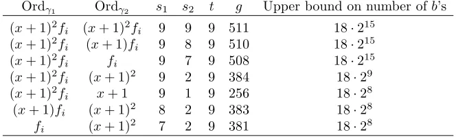
JC(F2) can be solved much faster than the 2127 time it would take using Pollard’s rho method, the gGHS attack is indeed effective for some elliptic curves whenℓ= 127 andn= 254. The vulnerable b’s, and upper bounds on their numbers, are listed in Table 2. In total, there are at most 221
Table 2. List of vulnerable b= (γ1γ2)2 for the case ℓ= 127, n= 254, q = 2.
Ordγ1 Ordγ2 s1 s2 t g Upper bound on number ofb’s (x+ 1)2f
i (x+ 1)2fi 9 9 9 511 18·215 (x+ 1)2f
i (x+ 1)fi 9 8 9 510 18·215 (x+ 1)2f
i fi 9 7 9 508 18·215 (x+ 1)2f
i (x+ 1)2 9 2 9 384 18·29 (x+ 1)2f
i x+ 1 9 1 9 256 18·28 (x+ 1)fi (x+ 1)2 8 2 9 383 18·28
fi (x+ 1)
2
7 2 9 381 18·28
vulnerable b’s. As in the n = 127 case, the number of isogeny classes that contain at least one vulnerable curve is at most 221/254 ≈213. Hence the probability that a randomly selected GLS curve has a vulnerable curve in its isogeny class is at most 213/2127 ≈ 1/2114, which is certainly negligible. Furthermore, one can efficiently verify that there is no vulnerable curve isogenous to a given GLS curve.
4.4. Summary. We have shown that GLS curves overF22ℓ withℓprime,ℓ∈[80,256], andℓ6= 127,
are not vulnerable to the generalized GHS Weil descent attack. Moreover, the probability that a randomly selected GLS curve over F2254 is vulnerable (or isogenous to a vulnerable curve) is
negligibly small, and in any case there is an efficient check that can be performed to rule out this possibility. Hence, GLS curves over F22ℓ with ℓ prime can be easily selected so that the fastest
attack known on the DLP is Pollard’s rho method.
5. Comparisons
We examine point multiplication on GLS curvesE′/F
22ℓ :Y2+XY =X3+a′X2+band random
curves E/F2n : Y2+XY = X3 +aX2+b (where n ≈ 2ℓ). For the case of random curves, we
at random subject to the requirement that #E(F2n) =hr where h is 2 or 4 (depending on Tr(a))
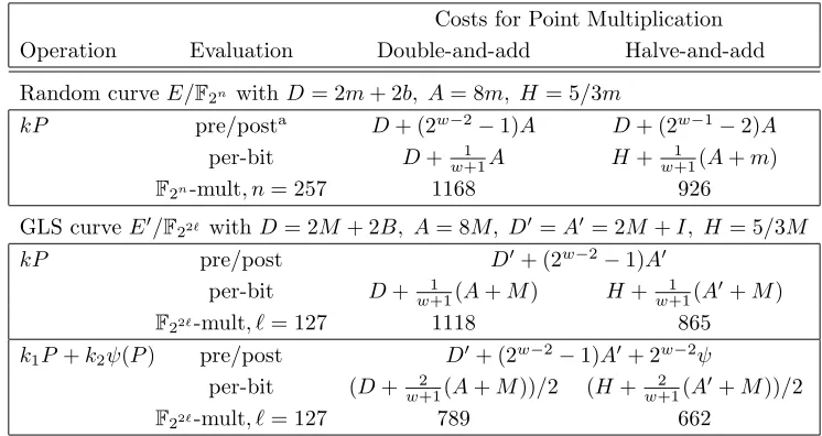
and r is prime; without loss of generality we may assume that a ∈ {0,1}. Table 3 summarizes point multiplication costs when parameters have been chosen compatible with the corresponding method, whereA′ and D′ denote cost of affine-coordinate addition and doubling, respectively, on the GLS curve. This section discusses assumptions and recent formulae improvements relative to the table, and highlights computational and practical differences between the curves and methods.
Table 3. Estimates for point multiplication on random curves E/F2n and GLS
curves E′/F
22ℓ. Multiplication costs for F2n and F22ℓ are denoted by m and M,
respectively. Inversion cost in F22ℓ is denoted by I. Costs for multiplication by
curve parameter b (or √b) for each curve are denoted by b and B, estimated at m/2 andM/3;ψdenotes the cost of applying the endomorphism. The costs in field multiplications usew = 5, I = 6M, ψ=M, and scalar bitlengths 256 and 253 for E and E′, resp.
Costs for Point Multiplication Operation Evaluation Double-and-add Halve-and-add
Random curveE/F2n withD= 2m+ 2b, A= 8m, H= 5/3m kP pre/posta D+ (2w−2
−1)A D+ (2w−1
−2)A
per-bit D+ 1
w+1A H+ 1
w+1(A+m)
F2n-mult, n= 257 1168 926
GLS curve E′/F22ℓ withD= 2M+ 2B, A= 8M, D′=A′= 2M+I, H= 5/3M
kP pre/post D′+ (2w−2
−1)A′
per-bit D+ 1
w+1(A+M) H+ 1
w+1(A′+M)
F22ℓ-mult, ℓ= 127 1118 865 k1P+k2ψ(P) pre/post D′+ (2w−2−1)A′+ 2w−2ψ
per-bit (D+ 2
w+1(A+M))/2 (H+ 2
w+1(A′+M))/2
F22ℓ-mult, ℓ= 127 789 662 a
Halve-and-add post-evaluation is multiple-accumulator fixup for right-to-left method.
5.1. Random curves. Fong et al. [7] compared point multiplication via doubling-based and halving-based methods on random curves with a = 1, with operation count and experimental data strongly favouring halving. Since then, formula improvements due to Kim and Kim [20] offer a significant acceleration to point doubling in the scenario where halving applies, namely a = 1 with a modest amount of per-curve precomputation permitted.3
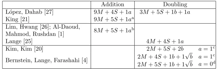
Table 4 summarizes the costs of point addition and doubling in L´opez-Dahab coordinates with various formulae and parameters. The significance of the Kim and Kim result is that total multipli-cations for doubling remain unchanged from earlier formulae, but the number of multiplimultipli-cations by curve parameter bis now 2 rather than 1. Since these formulae do not accelerate typical halving-based methods, we are interested in a revised doubling vs. halving comparison when precomputation significantly reduces the cost of multiplication by b. The comparison against halving is not quite
Table 4. Point operation cost for mixed-coordinate additions and projective dou-blings, where the projective point (X : Y : Z) corresponds to the affine point (X/Z, Y /Z2). M and S denote the costs of field multiplication and squaring, resp., and a,b,√b denote the cost of multiplication by the corresponding curve parame-ters.
Addition Doubling L´opez, Dahab [27] 9M+ 4S+ 1a 3M + 5S+ 1b+ 1a
King [21] 9M+ 5S+ 1aa
Lim, Hwang [26]; Al-Daoud,
Mahmod, Rushdan [1] 8M+ 5S+ 1a
b
Lange [25] 4M + 4S+ 1a
Kim, Kim [20] 2M+ 5S+ 2b a= 1c
Bernstein, Lange, Farashahi [4] 2M+ 4S+ 1b+ 1 √
b
2M+ 5S+ 1b+ 1√b
a= 1c
a= 0d
a
ProvidesXZandZ2
for subsequent double.b
ProvidesZ2
for subsequent double.
c
AssumesZ2
chained. d
AssumesXZ andZ2
chained.
as straightforward as it appears, since there is a one-multiplication “penalty” on essentially every point addition due to conversion fromλ-coordinates. However, thea= 1 formula for doubling does not pay this penalty, and this is the comparison that is most meaningful in the present context.
The counts in terms of field multiplication in Table 3 assume that field representations can be selected where square roots are inexpensive, in which case the halving step is dominated by a multiplication and the cost of the quadratic solver. In the modest-storage scenario with fields of interest in this paper, we assume that a point halving can be done in 5/3 the time of a field multiplication (so H ≈ 53m), and that multiplication by a constant with precomputation requires half the time of a general multiplication (sob≈√b≈m/2). Under these assumptions, Table 3 gives a factor 1.26 advantage to the halving-based approach on E. This is smaller than the factor 1.41 estimate in [7] where the L´opez-Dahab doubling formulas were used without off-line precomputation (but halving was estimated at a higher two-multiplication cost).
5.2. GLS curves. The GLS curvesE′/F
22ℓ :Y2+XY =X3+a′X2+b are “small parameter” in
the sense thatb∈F2ℓ anda′ can be chosen arbitrarily subject to the trace requirement Tr′(a′) = 1.
Compared to the random curves, multiplication by the corresponding curve parametersbor√bis a smaller fraction of the cost of a general multiplication. We can choosea′ so that multiplication by a′ is inexpensive; however, the GLS curves are trace-1 but nota′ = 1. The Kim and Kim formula for point doubling does not apply, but the techniques fora= 0 in the formula of Bernstein-Lange-Farashahi can be adapted as follows. To find 2P = (x3, y3) for P = (x, y) ∈ {−/ P,∞}, write the affine formulae as x3 =x2+b/x2 and y3=x2+ (λ+ 1)x3 where λ=x+y/x. Then
y3 =x2+
x2+y+x x
x4+b x2
= x
6+x(y2+y+x)(x4+b)
x4
and, as in (part of) Kim and Kim, the substitutionx6= (y2+xy+a′x2+b)2 from the curve equa-tion is used and the result written in L´opez-Dahab projective form (U3, V3, W3). Straightforward arithmetic gives thea= 0 Bernstein et al. formulae [4] but with the addition ofa′(a′T
Unlike Kim and Kim, the “two multiplications by constants” a = 0 Bernstein et al. formulas (and those adapted here for GLS) chain the quantity XZ in point doubling. The consequence can be similar to the point-halving method, where a point addition has a “penalty” of an extra multiplication. There is also multiplication by both b and √b in point doubling, although (as in Kim and Kim) this can be done via two multiplications bybat the cost of an extra squaring.
The GLV technique also has a precomputation penalty in the sense that there are now two inputs P and ψ(P) for which precomputation is required. If width-w NAF methods are employed, then the basic issue is that precomputation is used less efficiently when interleavingk1P andk2ψ(P). In practice, this penalty is small unless constraints limit the amount of precomputation to less than four points. Further, the precomputation involving ψ(P) can be obtained from that forP sinceψ is inexpensive compared to point addition. For suitable a′,ψ can be essentially free, in which case the table forψ(P) can be omitted and the values obtained on-demand from the table for P.
The Tr′(a′) = 1 condition on the GLS curves is favourable to point halving techniques (as discussed for random curves). The GLV and point halving techniques can be combined, with scalar recoding performed as follows. Assumer≈22ℓ and letk′ = 2ℓkmodr. Findk′ ≡k′
1+k′2λ (modr) via the usual GLV technique, givingk′
i of expected length approximatelyℓ. Thenki←k′i/2ℓ gives k ≡k1+k2λ (modr) with ki in essentially the form we seek, other than a few terms which will
involve doubling in point multiplication.
Finally, we note that the quadratic extension in GLS is attractive in the sense that operations in
F22ℓ reduce to operations inF2ℓ. In particular, precomputation for the quadratic solver can require
less storage than in the random curve case, and inversion inF22ℓ is reduced to three multiplications
and an inversion in F2ℓ. This inversion is likely to be sufficiently inexpensive that point addition
can be done in affine coordinates (and so halving-based methods can run entirely in affine).
5.3. Additional accelerations. Two types of accelerations are suggested by the GLS technique and the improved Kim and Kim doubling formulas that exploit precomputation. We briefly consider the effects of specializing curve parameters for random curvesEand for GLS curvesE′(where GLS has already forced a specialization ofb, namelyb∈F2ℓ). We also examine precomputation strategies
that offer less dramatic acceleration than those involving curve parameters, but are similar in the sense that they can re-use tables across point operations.
Specialized curve parameters. Since the GLS curves E′ are special in the sense that b ∈ F 2ℓ, we
consider specialized b for E and further specialization on E′ to speed point multiplication. At the extreme are Koblitz curves where b = 1, in which case different techniques apply and will not be considered here. For non-Koblitz curves, selecting specialized b will reduce the cost of doubling while the cost of halving remains the same. If b is of low hamming weight, for example, then multiplications by b and √b (given suitable field representation) in point doubling become inexpensive.
The overall improvement can be incremental if precomputation was already giving these mul-tiplications at 1/2 or 1/3 the cost of a general multiplication in E and E′, respectively, since the savings are diluted by point additions and other operations. However, if quite special bis accept-able and gives associated multiplication at, say, 1/8 the cost of general multiplication, then the estimates in Table 3 for E give 976 and 925 as the corresponding F2n-multiplication counts for
point multiplication onE via doubling and halving, resp., predicting that the two methods run at approximately the same time.
per-curve precomputation involving b and √b. King [21] describes re-use of multiplication tables within a point double or point addition, and this technique is examined in more detail in [3] (where it is called “sequential multiplications”) in the context of hyperelliptic curves where the arithmetic provides more opportunity to exploit the method.
King also describes a per-point precomputation strategy that applies in some point multiplication methods where there is a small set of points repeatedly accessed, as in left-to-right width-w NAF methods. The basic idea is to build tables for some of the field multiplications in point addition involving coordinates from the small set, since these coordinates will be used repeatedly. The cost of this precomputation is spread across the entire point multiplication rather than within a point operation, although admittedly the method is useful only for smallwand the gains are incremental. Further, the right-to-left windowing method in [7] used with halve-and-add (when inversions are expensive) precludes this acceleration, since the small set of fixed points is replaced by multiple accumulators.
6. Experimental results
For a concrete comparison, we implemented point multiplication methods on two curves, each at roughly the 128-bit security level. The target environment is “workstation-class” systems which do not have severe memory constraints. In this section, we describe the curves, implementation issues, development environment, and give timings.
We chose curve and field parameters to be compatible with the 128-bit security requirement and with the methods of interest. For random curves we chose n= 257, and for GLS curves we could not resist selecting ℓ= 127; if concerns about the security of elliptic curves over F2254 remain (see
§4), then ℓ= 131 would be a suitable alternative. For the random curve E, point halving and the best doubling formulas desirea= 1, and we chosebpseudo-randomly so that #E(F2257) = 2r with
r prime. The reduction polynomials were selected so that both reduction and square roots would be at low cost. The following table summarizes the selections.4
Curve a b Base Field Extension √x
E/F2n, n= 257 1 ∈F2257 F2[x]/(x257+x41+1) — x129+x21
E′/F22ℓ, ℓ= 127 u ∈F 2127 F
2[x]/(x127+x63+1) F2127[u]/(u2+u+1) x64+x32
For GLS, the choice a′ =u (compatible with the trace requirement) makes multiplication with a′ very inexpensive (comparable to selecting a∈ {0,1} for random curves). The correspondings in GLS (see §3.1) satisfies sq+s =u+ 1 and so ψ is essentially free. Curve parameter b∈ F2127
was chosen so that #E′(F
2254) = 2r where r is prime.
6.1. Implementation. The field and elliptic curve code was written in the C programming lan-guage, except for a small fragment in assembly to assist in finding the degree of a polynomial (for inversion). The big-number arithmetic required in the GLV method (to recode the scalar as k≡k1+k2λ (modr)) and in halving-based methods (to recode the scalar in base 1/2) is via the OpenSSL libraries.5 There are divisions required in GLV recoding, but these can be done per-curve so that only multiplications and shifts are involved per-scalar. Recoding for halving involves a single per-scalar modular reduction. Regardless, these operations are a minor portion of the overall cost of scalar multiplication.
4There are polynomialsx127
+r(x) giving two-term√xwhererhas smaller degree than inf(x) =x127
+x63
+ 1; we chosef since there are powers differing by a multiple of 64, and the higher degree ofr is not a significant factor in our environment. The root also is of advantageous form.
5The library at http://www.openssl.org is used in the communications tool OpenSSH, for example. Here, we are
Field multiplication. Base field multiplication is via comb methods [28]. Briefly, a common case of combing calculates c·dwith a single table of precomputation containing p·d for polynomials p of degree less than w for some small w (e.g., w = 4). The words of c are then “combed” w bits at a time to select the appropriate precomputed value to add at the desired location of the accumulator. These have been among the fastest methods for multiplication on general-purpose processors, and can be combined with shallow-depth Karatsuba-like techniques to control code expansion. However, going from 32- to 64-bit code can reduce the advantage of combing over the Karatsuba-down-to-word-multiplication used, for example, in the well-knownMiracllibrary [35].6 Nonetheless, combing appears to be fastest in our environment, and we combed on field elements with comb width 4. For 32- and 64-bit code, elements inF2257 can be represented in 8 or 4 words
along with an extra bit. Multiplication suffers only a small penalty by handling this bit separately. Elements in the extension fieldF2254 =F
2127[u]/(u2+u+ 1) are represented as a pair (a
0, a1) =
a0+a1uofF2127-elements, and extension field multiplication requires three multiplications in F 2127
via Karatsuba. Squaring requires two F2127-squarings. We expect similar multiplication times for F2254 and F
2257, although the practical comparison is not as clear as the mathematics indicates.
Roughly speaking, comb multiplication looks best when the machine register size is small compared to the number of words representing a field element. Depending on platform and n, it is possible that combing is fastest on field elements rather than via shallow-depth Karatsuba-like techniques combined with combing (essentially the technique for the extension field).
We used combing with windows of width 8 for multiplications by constants (band √b). This is double the window size used for general multiplication, and the precomputation of 256 elements (per constant) is off-line. Hence, the run time is expected to be approximately half the time of a general multiplication. A possible downside of combing is that compilers can be rather sensitive to the precise form of the code; e.g., some compilers do not optimize arrays as well as scalars, even when indices are known at compile-time. As a platform-dependent example, array dimensions and access order in a table-lookup method such as comb can mean 10% overall difference in multiplication due to the cost of addressing.
Inversion. Inversion is via a Euclidean-algorithm variant, and only limited optimization was per-formed. An assembly language fragment for Pentium-like systems was used to exploit a bitscan instruction (bsr) useful for speeding degree calculations. Inversion in F2254 was performed by
ele-mentary matrix methods costing threeF2127-multiplications and an inversion inF 2127.
Solving quadratics. Finding solutions to λ2+λ=c for trace-0 c in F
2257 was done via Algorithm
3.86 of [16] with 4-bit lookups in accumulation of half-traces. This technique is easier to implement for a given field than the small-table methods illustrated in [7], and uses less storage and has lower accumulation cost than the method used in [2]. The reduction polynomial x257+x41+ 1 gives especially clean and efficient code, although this choice builds the table from 84 half-trace computations rather than the 71 elements specified by this algorithm for x257+x12+ 1 (but the latter polynomial increases the cost of roots). The extra-digit storage-and-performance penalty noted for multiplication is avoided in the quadratic solver by not tracking the constant term.
Solutions inF2254 are found by reduction toF
2127 as follows. Forc=c
0+c1uwithci ∈F2127, solve
λ2+λ=c
1to getλ1, and then obtainλ0fromλ2+λ=c′0+Tr(c′0) wherec′0=c0+λ21 =c0+c1+λ1. The solution is thenλ0+ (λ1+ Tr(c′0))u.
6In personal communication, Julio L´opez reports comb variants that can better exploit certain processor
charac-teristics; in particular, his timings on an AMD Athlon64 are 35% faster onF21223 than timings from an Opteron in
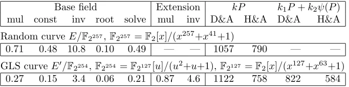
Table 5. Timings (in 103 cycles) on a 3.16 GHz Xeon with Sun C 5.9. Field opera-tion “const” denotes multiplicaopera-tion by a constant with precomputaopera-tion, and “solve” findsλgiven trace-0 c so thatλ2+λ=c. “D&A” is width-5 NAF double-and-add. “H&A” is width-5 NAF with right-to-left half-and-add on E [16, Algorithm 3.91] and affine additions on E′. The GLV decomposition is kP = k
1P +k2ψ(P) with width-5 NAF applied to k1 and k2.
Base field Extension kP k1P +k2ψ(P)
mul const inv root solve mul inv D&A H&A D&A H&A
Random curveE/F2257,F
2257 =F
2[x]/(x257+x41+1)
0.71 0.48 10.8 0.10 0.49 — — 1057 790 — —
GLS curveE′/F2254,F
2254 =F
2127[u]/(u2+u+1),F
2127 =F
2[x]/(x127+x63+1)
0.27 0.15 3.4 0.06 0.21 0.87 4.6 1122 758 822 584
Square-root computations are inexpensive with the choice of reduction polynomials f. Coeffi-cients corresponding to even and odd powers of x were extracted simultaneously by 8-bit lookup, and then √c = P
c2ixi +√xPc2i+1xi. Since the degree of √x is at most (degf + 1)/2 in our case, no reduction is required and finding a square root is less expensive than a squaring.
6.2. Performance comparisons. Timings in Table 5 were obtained on a Sun X4150, a 64-bit system built on the Intel Xeon processor (model 5460, 3.16 GHz). Roughly speaking, this processor family includes the Intel Core2 and the Athlon64 and Opteron from AMD, with similar instruction sets and timings. The compiler is Sun C 5.9, producing 64-bit objects.
The point multiplication times include the cost of scalar recoding (k≡k1+k2λ (modr) in GLV, and base 1/2 form of k in halving). A sequence of pseudo-random elements and scalars was used in the timings to preclude effects such as branch prediction that would not apply outside of the laboratory. As expected, field multiplication times forF2257 and F
2254 are roughly comparable. If
these times were the same, then Table 3 would predict that E′ is faster thanE for point multipli-cation in the non-GLV timings. The experimental data shows that E does better than predicted in this comparison, and the main reason is that the comb multiplier is more efficient there than on the subfieldF2127.
The GLV technique provides an acceleration of 27% and 23% for doubling- and halving-based methods on E′; as expected, the combination of GLV decomposition and point halving gives the best time. A comparison of interest is between E′ and E, and this is the comparison for prime fields in [10] where the acceleration from GLV is 16% for 64-bit code on an Intel Core2 and 30% on an 8-bit Atmel. The corresponding comparison for point halving methods in our case is 26%. While the comparison against E may indeed be the “right” one, it comes with a caveat that the measurement is polluted by differences in field multiplication times, a portion of which are due to programmer talent or lack thereof and vary by processor. A significant difference between the case for curves over prime fields from those over binary fields is the cost ratio of point addition to doubles. As rough approximations in the scenarios of interest, the ratio in the prime field case is 11/8, while the ratio for binary fields is 8/4. Since the GLV technique reduces doubles but not additions, the opportunity for improvement is apparently larger for prime fields.
7. Conclusions
point halving. Recent improvements to doubling formulae have narrowed the performance gap be-tween the doubling- and halving-based techniques, although halving retains a significant advantage provided a threshold amount of per-field precomputation is available for the quadratic solver. On the other hand, if fairly specialized curve parameters are acceptable, then the analysis shows that the new formulae can eliminate most of the advantage of halving.
References
[1] E. Al-Daoud, R. Mahmod, M. Rushdan and A. Kilicman, “A new addition formula for elliptic curves over
GF(2n)”,IEEE Transactions on Computers, 31 (2002), 972–975.
[2] R. Avanzi, “Another look at square roots (and other less common operations) in fields of even characteristic”, Selected Areas in Cryptography – SAC 2007, Lecture Notes in Computer Science, 4876 (2007), 138–154. [3] R. Avanzi and N. Th´eriault, “Effects of optimizations for software implementations of small binary field
arith-metic”,Arithmetic of Finite Fields – WAIFI 2007, Lecture Notes in Computer Science, 4547 (2007), 69–84. [4] D. Bernstein, T. Lange and R. Farashahi, “Binary Edwards curves”, Cryptographic Hardware and Embedded
Systems – CHES 2008, Lecture Notes in Computer Science, 5154 (2008), 244–265.
[5] C. Diem and E. Thom´e, “Index calculus in class groups of non-hyperelliptic curves of genus three”,Journal of Cryptology, 21 (2008), 593–611.
[6] A. Enge and P. Gaudry, “A general framework for subexponential discrete logarithm algorithms”, Acta Arith-metica, 102 (2002), 83–103.
[7] K. Fong, D. Hankerson, J. L´opez and A. Menezes, “Field inversion and point halving revisited”,IEEE Transac-tions on Computers, 53 (2004), 1047–1059.
[8] S. Galbraith, “Constructing isogenies between elliptic curves over finite fields”, LMS Journal of Computation and Mathematics, 2 (1999), 118–138.
[9] S. Galbraith, F. Hess and N. Smart, “Extending the GHS Weil descent attack”, Advances in Cryptology – EUROCRYPT 2002, Lecture Notes in Computer Science, 2332 (2002), 29–44.
[10] S. Galbraith, X. Lin and M. Scott, “Endomorphisms for faster elliptic curve cryptography on general curves”, Cryptology ePrint Archive: Report 2008/194, 2008. Available from http://eprint.iacr.org/2008/194.
[11] R. Gallant, R. Lambert and S. Vanstone, “Faster point multiplication on elliptic curves with efficient endomor-phisms”,Advances in Cryptology – CRYPTO 2001, Lecture Notes in Computer Science, 2139 (2001), 190–200. [12] P. Gaudry, F. Hess and N. Smart, “Constructive and destructive facets of Weil descent on elliptic curves”,
Journal of Cryptology, 15 (2002), 19–46.
[13] S. Gueron and M. Kounavis. “Carry-less multiplication and its usage for computing the GCM mode”, white paper, Intel Corporation, 2008. Available from http://softwarecommunity.intel.com/articles/eng/3787.htm. [14] S. Gueron and M. Kounavis. “A technique for accelerating characteristic 2 elliptic curve cryptography”, InFifth
International Conference on Information Technology: New Generations (ITNG 2008), IEEE Computer Society, 2008, 265–272.
[15] D. Hankerson, A. Menezes, and M. Scott, “Software implementation of pairings”,Identity-Based Cryptography, edited by M. Joye and G. Neven, IOS Press, to appear.
[16] D. Hankerson, A. Menezes and S. Vanstone,Guide to Elliptic Curve Cryptography, Springer, 2003.
[17] F. Hess, “Generalising the GHS attack on the elliptic curve discrete logarithm problem”, LMS Journal of Computation and Mathematics, 7 (2004), 167–192.
[18] I. Iijima, K. Matsuo, J. Chao and S. Tsujii, “Construction of Frobenius maps of twists elliptic curves and its ap-plication to elliptic scalar multiap-plication”,Proceedings of the 2002 Symposium on Cryptography and Information Security – SCIS 2002, Japan, 2002.
[19] D. Jao, S. Miller and R. Venkatesan, “Do all elliptic curves of the same order have the same difficulty of discrete log?”,Advances in Cryptology – ASIACRYPT 2005, Lecture Notes in Computer Science, 3788 (2005), 21–40. [20] K. Kim and S. Kim, “A new method for speeding up arithmetic on elliptic curves over binary fields”, Cryptology
ePrint Archive: Report 2007/181, 2007. Available from http://eprint.iacr.org/2007/181.
[21] B. King, “An improved implementation of elliptic curves overGF(2n) when using projective point arithmetic”,
Selected Areas in Cryptography – SAC 2001, Lecture Notes in Computer Science, 2259 (2001), 134–150. [22] B. King and B. Rubin, “Improvements to the point halving algorithm”,Australasian Conference on Information
Security and Privacy – ACISP 2004, Lecture Notes in Computer Science, 3108 (2004), 262–276.
[24] N. Koblitz, “CM-curves with good cryptographic properties”,Advances in Cryptology – CRYPTO ’91, Lecture Notes in Computer Science, 576 (1992), 279–287.
[25] T. Lange, “A note on L´opez-Dahab coordinates”,Tatra Mountains Mathematical Publications, 33 (2006), 75-81. Also available from http://eprint.iacr.org/2004/323.
[26] C. Lim and H. Hwang, “Speeding up elliptic scalar multiplication with precomputation”,Information Security and Cryptology ’99, Lecture Notes in Computer Science, 1787 (2000), 102–119.
[27] J. L´opez and R. Dahab, “Improved algorithms for elliptic curve arithmetic inGF(2n)”,Selected Areas in
Cryp-tography – SAC ’98, Lecture Notes in Computer Science, 1556 (1999), 201–212.
[28] J. L´opez and R. Dahab, “High-speed software multiplication inF2m”,Progress in Cryptology – INDOCRYPT
2000, Lecture Notes in Computer Science, 1977 (2000), 203–212.
[29] M. Maurer, A. Menezes and E. Teske, “Analysis of the GHS Weil descent attack on the ECDLP over characteristic two finite fields of composite degree”, LMS Journal of Computation and Mathematics, 5 (2002), 127–174. [30] A. Menezes and M. Qu, “Analysis of the Weil descent attack of Gaudry, Hess and Smart”,Topics in Cryptology
– CT-RSA 2001, Lecture Notes in Computer Science, 2020 (2001), 308–318.
[31] A. Menezes, P. van Oorschot and S. Vanstone,Handbook of Applied Cryptography, CRC Press, 1996.
[32] B. M¨oller, “Algorithms for multi-exponentiation”,Selected Areas in Cryptography – SAC 2001, Lecture Notes in Computer Science, 2259 (2001), 165–180.
[33] J. Muir and D. Stinson, “Minimality and other properties of the width-w nonadjacent form”,Mathematics of Computation, 75 (2006), 369-384.
[34] R. Schroeppel, “Automatically solving equations in finite fields”, US patent application No. 09/834,363, filed April 12, 2001.
[35] M. Scott,MIRACL – Multiprecision Integer and Rational Arithmetic C Library, http://www.computing.dcu.ie/ ∼mike/miracl.html.
[36] J. Solinas, “Efficient arithmetic on Koblitz curves”,Designs, Codes and Cryptography, 19 (2000), 195–249.
Department of Mathematics & Statistics, Auburn University, Auburn, Alabama 36849 USA E-mail address: [email protected]
Department of Combinatorics & Optimization, University of Waterloo, Waterloo, Ontario N2L 3G1 Canada
E-mail address: [email protected]
Department of Combinatorics & Optimization, University of Waterloo, Waterloo, Ontario N2L 3G1 Canada