Suitable Impedance Boundary Condition Applied
to the Enhancement of the Electric Field Radiated by a High
Frequency Surface Wave Radar
Nicolas Bourey1, *, Florent Jangal2, Muriel Darces1, Marc H´elier1, and Philippe Pouliguen3
Abstract—Efficiency of high frequency surface wave radars may be improved by inserting a metamaterial in the vicinity of transmitting antennas that will reinforce the propagation of surface waves. This paper deals with the first and second order derivations of the surface impedance boundary conditions (IBC) applied to model such a metamaterial, which is equivalent to a bounded ground with a low negative permittivity. The goal of this paper is to extend an approach previously based on the classical Leontovich IBC which is usually restrained to high permittivity grounds. As shown here, a simplification in the expression of the surface impedance is possible in the case of a planar and homogeneous surface. That allows to have a first order impedance boundary condition substituted for the required second order impedance boundary condition.
1. INTRODUCTION
High Frequency Surface Wave Radars (HFSWR) are currently deployed worldwide [1, 2] and particularly in the European Union [3] as a part of the Integrated Maritime Surveillance Systems (IMSS). These systems aim to bring global and operational means for maritime security and surveillance [4]. Those radars are considered as an optimum and low cost solution for monitoring the Exclusive Economic Zone. HFSWR are based on the property of high frequency waves to be propagated beyond the line-of-sight. Indeed, at those frequencies (i.e., from 3 MHz to 30 MHz), electromagnetic waves have the ability to be guided over the surface of the sea with reasonable losses. Fig. 1(a) shows a biconical antenna used for Onera’s demonstrator of the HFSWR located at Levant Island in France. We can see in Fig. 1(b) typical tracking results in the Mediterranean sea.
Today, a substantial effort is required to increase the efficiency of HFSWR while reducing their cost. During the last decade, improvements of HFSWR systems have dealt with compactness [5], clutter removal [6] and architecture or detection scheme [7]. Actually, most of the electromagnetic power of transmitting antennas is radiated towards the sky and a minor part of it is radiated at low elevation angle. Therefore, an increase of the surface wave power radiated by the transmitting antennas is an essential contribution to improve the efficiency of HFSWR. But this improvement may go through the use a low negative permittivity medium which is not properly characterized by the standard approach. Hence, there is still an issue regarding this solution since the simulation results could be a calculation artifact [8].
In order to clarify the surface wave improvement using such a metamaterial, we propose an accurate analytic formulation to compute the electromagnetic field radiated by the transmitting antennas whatever the permittivity of the antenna ground is. We have mainly based our approach on the
Received 18 May 2018, Accepted 25 June 2018, Scheduled 10 July 2018 * Corresponding author: Nicolas Bourey ([email protected]).
(a) (b)
Figure 1. (a) A biconical antenna and (b) results of tracking in the Mediterranean sea.
works published by Karp and Karal [9]. They have derived a decomposition of the electromagnetic field radiated by a magnetic line source located above a plane structure. We have also taken into account the results obtained by Kane and Karp [10] who have introduced a second order impedance boundary condition. The latter approach is not limited to large permittivity values like the Leontovich one [11].
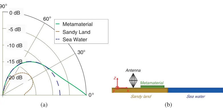
In Section 2, we show that a metamaterial can effectively propagate a strong surface wave. In Section 3, we describe the geometry of the studied configuration and explain the principle of surface impedance boundary condition. In Section 4, we derive the field radiated by an infinite line source of vertical electric Hertzian dipoles, using a first order Impedance Boundary Condition (IBC), when the source is over a soil with low negative permittivity. In Section 5, we recall the second order IBC which allows to consider ground with a permittivity close to unity. Finally, we will draw a conclusion.
2. ENHANCED SURFACE WAVE
(a) (b)
Sandy land Sea water
0 dB 90
Metamaterial Sandy Land Sea Water -5 dB
-10 dB
-15 dB
-20 dB
60
30
0 o
o
o
o y x
z
Antenna
Metamaterial
Figure 2. (a) shows the distribution of the vertical component of the electric field radiated by a Hertzian dipole located over different grounds, at 10 MHz and at 50 m from the antenna and (b) depicts the side view of the new HFSWR configuration.
3. IMPEDANCE BOUNDARY CONDITIONS
During the last century, many authors [11, 15] tried to derive the field radiated by a Hertzian dipole over a good conductor and developed an IBC as a substitute of the conductor. In [11] the main assumptions are that the soil is plane and exhibits a permittivity with a large magnitude. This last point leads to neglect the second order variation of the field along the interface. In the same time, Rytov [15] extended this formulation of IBC for a curved surface but still assuming a ground with a large permittivity. In 1959, Karp and Karal [9] proposed a General Impedance Boundary Condition (GIBC) to model a dielectric medium which can propagate more than one surface wave as, for example, a dielectric slab with a large thickness. But this derivation has been performed considering a magnetic line source which has not the characteristics of the antenna used in the HFSWR applications. The condition has also been used in [16] to study the problem of a planar metal-backed uniform dielectric layer. Kane and Karp [10] applied the second order GIBC to study the reflection of plane waves by a soil with a permittivity close to unity. In consequence, starting from the results obtained by Kane, Karal and Karp [9, 10], we will describe, in this section, the required steps to establish the first and second IBC in case of an infinite line source of vertical Hertzian dipoles. The electromagnetic behaviour of such a source is in better relation to that of the antennas used in HFSWR.
3.1. Geometry
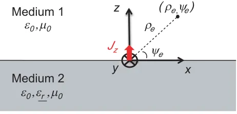
The geometry is depicted in Fig. 3 in a Cartesian coordinate system with a time dependence e−iωt. A plane interface separates the two media atz= 0. Medium 1 in the upper side (z >0) is air characterized by ε0, the vacuum permittivity, andμ0, the vacuum permeability. Medium 2 in the lower side (z <0) is a dielectric medium whose relative complex permittivity is εr, expressed as:
εr=εrr+ iωε0σ (1)
where ω is the angular frequency; εrr and σ are respectively the real part of the relative permittivity
and the conductivity of the medium.
We consider an infinite line source of vertical electric Hertzian dipoles located along the y axis (x=z= 0). It carries a current density in A/m2:
Jz =Ieδ(x)δ(z) (2)
y x Medium 1
Medium 2
z
J
zψ
eρ
eε ,
0μ
0(
ρ
e,ψ
e)
ε ,
rμ
0ε ,
0Figure 3. Geometry under consideration.
The geometry is invariant in y, and hence the source radiates a Transverse Magnetic (TM) mode of propagation. As we are interested in the surface wave mode, we will focus on the propagation along thex axis. Thus the following assumptions are considered:
∂Ex
∂y = 0, ∂Ez
∂y = 0, ∂Hy
∂y = 0 (3)
Ey = 0, Hx = 0, Hz = 0 (4)
The next step consists in solving the Helmholtz equation inHy which can be expressed in medium 1
as:
∂2 ∂x2 +
∂2 ∂z2 +k
2 0
Hy(x, z) = ∂J∂xz (5)
where k0 is the vacuum wave number and the right part of the equation stands for the source. From Maxwell-Amp`ere’s and Maxwell-Faraday’s equations, we can express the components of the electric field as a function of the y-component of the magnetic field:
Ex = +
1 iωε0
∂Hy
∂z (6)
Ez = −
1 iωε0
∂Hy
∂x −Jz
(7)
It is not necessary to express the Helmholtz equation in medium 2 as the fields in medium 1 can be derived by applying an IBC at z= 0.
3.2. First and Second Order IBC Derivation
The surface impedance concept enables to replace medium 2 by an IBC which reduces the complexity of the computation. This condition is an approximated relation between the tangential components of the electric and magnetic fields at the interface (z= 0).
The first author who introduced the IBC is Leontovich [11]. Assuming that |εr| 1, this first
order condition can be expressed as:
ˆ
n×E =Zˆn×
ˆ
n×H
(8)
where ˆn is the outgoing normal to the interface and Z =εμ0
0εr is the impedance of medium 2. In our
case, Equation (8) is reduced to:
Ex =−ZHy (9)
Combining Equations (6) and (9), the first order IBC can be expressed as:
∂ ∂z +λs
whereλs is an imaginary wave number along thez axis that can be written as:
λs= iωε0Z = ik0
1
εr
(11)
To obviate the constrain on the magnitude of the permittivity, Kane and Karp [10] introduced a second order IBC in 1964. This condition is an expansion of the field components in Taylor series [17] that can be written as:
Λs2 ∂ 2
∂x2 + ∂ ∂z +λs
Hy(x, z) = 0, z= 0 (12)
where
Λs2 =
i 2k0(εr)3/2
(13)
Considering Equations (7), (10) and (12), we can include both boundary conditions in one General IBC, named GIBC, which depends only on the normal component of the electric field and can be written as:
N
m=0 am
(ik0)m
∂m
∂zmEz(x, z) = 0, z= 0 (14)
whereN is the order of the IBC. We have gathered the different types of conditions in Table 1.
Table 1. Order of surface impedance condition.
N Name of condition Nature of soil 0 Perfect Electric Conductor Condition PEC 1 Leontovich Boundary Condition |εr| 1
2 High Order Condition |εr|>1
4. FORMULATION FOR A FIRST ORDER IBC
As mentioned before, the IBC has been extensively studied for magnetic line source which obviously does not match our needs for surface wave propagation. Here after we have derived the IBC using an infinite line source of vertical electric Hertzian dipoles. We can derive the result in closed-form by using an approach similar to that applied to a horizontal magnetic line source [9]. The decomposition of the field is performed by applying an IBC at the interface. Firstly, we will start with the Leontovich Condition (10) and compare our results to the results generated by the full-wave commercial software FEKO. Secondly, we will improve the first order IBC by a slight modification to consider grounds with a permittivity close to unity.
The magnetic field can be decomposed in three terms as follows:
Hy(x, z) =Hy(d)(x, z) +Hy(r)(x, z) +Hy(sur)(x, z) (15)
whereHy(d)(x, z) andHy(r)(x, z) are respectively the direct and reflected fields whose summation defines
the sky wave mode, calledHy(sky)(x, z). Hy(sur)(x, z) is the surface wave mode.
4.1. Formulation
To express the magnetic field radiated by an infinite line source of electric vertical Hertzian dipoles, we solve the Helmholtz Equation (5) and use the Leontovich Condition (10) to replace medium 2.
∂ ∂z +λs
Hy(x, z) =v(x, z) (16)
One particular solution is:
Hyp(x, z) =e−λsz z
−∞
eλsηv(x, η)dη (17)
The auxiliary functionv(x, z) is a solution of the Helmholtz equation and can be written as:
v(x, z) = ik0 4
∂ ∂z
H1(1)(k0ρe) cosψe
(18)
whereH1(1) is the Hankel function of order one of the first kind; ρe= √
x2+z2 is the distance between
the origin and the observation point; cosψe= √x2x+z2.
We combine Equations (17) and (18), and integrate by parts to obtain the sky wave mode:
Hy(sky)(x, z) = +ik0 4 H
(1)
1 (k0ρe) cosψe−
ik0λs
4 e −λsz
z
−∞
eλsηH(1)
1 (k0ρη) cosψηdη (19)
whereρη =
x2+η2 and cosψ
η =√x2x+η2.
The surface wave mode is the solution of the homogeneous Helmholtz Equation (5) and is obtained from a separation of variables. The solution can be written as:
Hy(sur)(x, z) =Aeikzzei√k02−kz2|x| (20)
where kz is the wave number along the z axis. Now, we proceed by determining the expressions of kz
and A. Firstly, we substitute the first order IBC in Equation (10) into Equation (20), and the value of
kz can be expressed as:
kz= iλs (21)
Secondly, we apply the continuity condition of the tangential component Ex of the electric field
across the linex= 0 and the value of A can be expressed as:
A= λs
2 (22)
The total magnetic field is the sum of Equations (19) and (20). It can be expressed as:
Hy(x, z) = +
ik0
4 H
(1)
1 (k0ρe) cosψe−
ik0λs
4 e −λsz
z
−∞
eλsηH(1)
1 (k0ρη) cosψηdη+ λ2se−λszei √
k02+λs2|x|
(23) Looking at Equation (23) the first term is the direct field. The second term is a continuous spectrum and corresponds to the reflected field. These two terms constitute the sky wave contribution to the total magnetic field. The third term can be identified as a surface wave propagating along the interface.
4.2. Numerical Results
In this section and in the forthcoming results, we are interested in the decay of the magnetic field along the interface (z= 0). We will compare the surface wave contribution with the total magnetic field. Two kinds of soil will be considered: one with a large permittivity and one with a low permittivity.
perfect agreement for the surface wave contribution as well as for the total magnetic field. Nevertheless, Norton’s formulation is not valid when the soil has a permittivity close to the unity.
In order to validate our approach with that kind of soil, we have compared our results with those obtained through a full-wave simulation performed with the commercial software FEKO. To perform the computation with FEKO, we have simulated a quasi infinite line source, defined with 600 vertical electric Hertzian dipoles, each dipole having a length equal toλ/300, the gap between each dipole being of λ/5.
Figure 4(a) shows the decay of theHy component when medium 2 is sea water. This medium has
a large value of permittivity (εrr = 81, σ= 5 S/m). In such a case, first order and FEKO solutions are
identical. We can also notice that the contribution of the surface wave is entirely masked as the total magnetic field is equal to the sky wave contribution whatever the distance is. This complies with the usual propagation properties of wave over a soil with a positive permittivity.
0 5 10 15
distance [km] -30
-25 -20 -15 -10 -5 0
|H
y
| [dBA/m]
Feko
Surface - 1st order
Total - 1st order
0 200 400 600 800 1000
distance [m] -70
-60 -50 -40 -30 -20 -10 0
|H
y
| [dBA/m]
Feko
Surface - 1st order
Total - 1st order
(a) (b)
Figure 4. Decay of the magnetic field radiated by an infinite line source of Hertzian dipoles over soils (a) with a large positive permittivity and (b) with a low negative permittivity at 10 MHz. (a)εrr= 81;
σ= 5 S/m. (b) εrr =−2;σ= 0.001 S/m.
On the contrary, when the line source is located over a ground with a negative permittivity, as shown in Fig. 4(b), there are two modes of propagation depending on the distance to the source. Close to it, the total magnetic field is equal to the surface wave, and at a larger distance the total magnetic field is equal to the sky wave. Similar results have been observed on a metallic plane at optical frequencies for which the interface behaves like a metamaterial [19]. In this case, the first order and FEKO solutions are not identical. Indeed, the first order solution is not accurate when the soil has a permittivity close to the unity.
4.3. Extension of the First IBC Validity Range
As shown previously, the Leontovich condition is not applicable to a ground characterized by a low permittivity. But assuming that the soil is planar and homogeneous, the first order IBC can be improved by a slight modification.
Considering only the surface wave, the solution in medium 1 for the magnetic field is already known and expressed in Equation (20):
Hy1(x, z) =A1eikz1zeikxx (24)
In medium 1, the tangential componentEx of the electric field is easily deduced from Equation (6)
and can be expressed as:
Ex1(x, z) =A1kz1 ωε0e
In medium 2, the magnetic and electric fields are given by:
Hy2(x, z) = A2e−ikz2zeikxx (26)
Ex2(x, z) = −A2 kz2 ωε0εre
−ikz2zeikxx (27)
At the interface (z= 0), the continuity ofHy imposes that A1 =A2 and then the continuity ofEx
implies that:
kz1 kz2
= 1
εr
(28)
From the dispersion relation in medium 1 (k02 =kx2+k2z1) and in medium 2 (εrk02 =k2x+k2z2), we
find the expression ofkx:
kx =k0
εr
1 +εr
(29)
and then the expression of kz2:
kz2 =k0
εr2
1 +εr
(30)
The general expression of the surface impedance in TM mode is given by Equation (9) at the interface (z= 0). Then, we can deduce the expression of the modified surface impedanceZmod as:
Zmod= kz2
ωε0εr
(31)
We combine Equations (30) and (31), and the modified surface impedance can also be written as:
Zmod= k0
ωε0
1 1 +εr
(32)
and the modified imaginary wave number along thez axis that can be written as:
λsmod = ik0
1 1 +εr
(33)
Now we replace λs by λsmod in Equation (23) and obtain the new expression of the magnetic field
radiated by an infinite line source of Hertzian dipoles using a modified first order solution.
4.4. Numerical Results
In this section, we are interested in the comparison between the first order solution, the first order modified solution and the FEKO’s one in Fig. 5. We compare the values of the total magnetic field obtained when using this approach and the second order IBC, in the cases of soils with low negative permittivities (εrr = −2 or −4 and σ = 0.001 S/m). In both cases, we have a very good agreement
between the full-wave results and the first order modified ones. So, it appears that this modified surface impedance can be applied as a substitute of the second order IBC in the case of a planar and homogeneous interface.
Nevertheless, if the soil is not planar, for example to simulate a realistic rough surface of the sea, the first order modified solution cannot be applied. It is the reason why, in the next section, we have extended our formulation using a second order IBC. It will also provide us with the opportunity to compare the second order results to the first order modified ones.
5. EXTENDED FORMULATION USING A SECOND ORDER IBC DERIVATION
0 500 1000 1500 2000 distance [m] -70 -60 -50 -40 -30 -20 -10 0 |H y | [dBA/m] Feko
Total - 1st order Total - 1st order mod
0 200 400 600 800 1000
distance [m] -70 -60 -50 -40 -30 -20 -10 0 |H y | [dBA/m] Feko
Total - 1st order Total - 1st order mod
(a) (b)
Figure 5. (a) and (b) Decay of the magnetic field radiated by an infinite line source of Hertzian dipoles over soils with low negative permittivities at 10 MHz. (a) εrr = −4; σ = 0.001 S/m. (b) εrr = −2;
σ= 0.001 S/m.
5.1. Formulation
Now, we use Equation (12) as the IBC. For calculation convenience, we switch to the Fourier domain to compute the magnetic field. The second order IBC in the Fourier domain can be written as:
∂ ∂z +γs
ˆ
Hy(s, z) = 0, z= 0 (34)
whereγs=λs−Λs2s2;sis the spectral variable associated to thex variable, and the symbol ˆdenotes
variable expressed in the Fourier domain. It can be noticed that the second order IBC has, in the Fourier domain, an expression similar to that of the first order in the spatial domain (10).
Then the Helmholtz equation becomes:
∂2 ∂z2 +K
2
ˆ
Hy(s, z) =−isδ(z) (35)
where K =k02−s2. Applying the same approach as the one used for the first order, we obtain the
sky wave mode in the Fourier domain that can be written as:
ˆ
Hy(sky)(s, z) = s 2K
⎛
⎝eiKz−γ
se−γsz z
−∞
eγsηeiKηdη ⎞
⎠ (36)
In the spatial domain, the sky wave mode is then given by:
Hy(sky)(x, z) = +ik0 4 H
(1)
1 (k0ρe) cosψe−
1 4π
+∞
−∞
sγse−γsz
k2 0−s2
z
−∞
eγsηei √
k02−s2ηdηeisxds (37)
The direct field does not depend on the choice of the IBC, then the first term is found equal to that of Equation (23).
As in the first order resolution, the surface wave mode is the solution of the homogeneous Helmholtz Equation (5) whose solution is given by Equation (20). We use the same approach to find A and kz
when applying the second order IBC of Equation (12) in Equation (20). Finally, they can be written as:
kz = iβs (38)
A = βs
where
βs=−
1±i
−1−4λsΛs2+ 4(k0Λs2)2
2Λs2
(40)
where the±sign refers to the sign of the real part of the ground permittivity. The total magnetic field can then be written as:
Hy(x, z) = +
ik0
4 H
(1)
1 (k0ρe) cosψe−
1 4π
+∞
−∞
sγse−γsz
k20−s2
z
−∞
eγsηei √
k20−s2ηdηeisxds + βs
2e
−βszei√k02+βs2|x|
(41)
5.2. Numerical Results
In this section, we are interested in the decay of the magnetic field along the interface (z= 0). We will compare the surface wave contribution with the total magnetic field given by the second order solution and FEKO’s one. Two kinds of soil have been considered.
The results shown in Fig. 6 are obtained over grounds with a negative permittivity (εrr = −2 or −4 andσ = 0.001 S/m) and all solutions are in very good agreement.
0 500 1000 1500 2000
distance [m] -70
-60 -50 -40 -30 -20 -10 0
|H
y
| [dBA/m]
Feko
Total - 1st order mod
Total - 2nd order
0 200 400 600 800 1000
distance [m] -70
-60 -50 -40 -30 -20 -10 0
|H
y
| [dBA/m]
Feko
Total - 1st order mod
Total - 2nd order
(a) (b)
Figure 6. (a) and (b) Decay of the magnetic field radiated by an infinite line source of vertical electric Hertzian dipoles over soils: with low negative permittivities at 10 MHz. (a) εrr =−4; σ = 0.001 S/m.
(b)εrr=−2;σ = 0.001 S/m.
Figure 7 shows, at two distances from the source, the influence of the real part of the permittivity on the relative discrepancies between the magnetic fields obtained with first and second order conditions. As expected with [10] closer is the permittivity to unity, larger is the relative error.
This section may be ended with two main conclusions. The first and the main one is that only a negative permittivity allows the propagation of a strong surface wave. The second one claims that, having a ground with a low permittivity, the Leontovich condition is questionable since it significantly differs from a higher order model.
! ! ! ! ! ! !
! !
-10 -8 -6 -4 -2
0 50 100 150 200
Relative permittivity of the medium
%
! 100 m
50 m ! !
!
!
!
! !
!
2 4 6 8 10
0 10 20 30 40 50
Relative permittivity of the medium
%
! 100 m
50 m
(a) (b)
Figure 7. Relative error between the magnetic fields obtained with first and second order conditions at 50 m and 100 m (a) with a negative real part of permittivity and (b) with a positive real part of permittivity.
6. CONCLUSION
To improve the performance of a HFSWR, it is possible to insert a metamaterial medium between the transmitting antennas and the sea in order to reinforce the propagation of strong surface waves [14]. Nevertheless, the design of such a material highlights the limits of accuracy of the standard IBC when a low permittivity medium is considered. In this paper, we have proposed an accurate and quite simple analytic formulation of the impedance boundary condition (IBC) derived from the first order IBC, suitable to compute the electromagnetic field radiated by the transmitting antennas over a ground with a low positive permittivity but also with a negative permittivity, which characterizes such a metamaterial medium. As needed, this approach leads to an electromagnetic field decomposed in three terms, the direct and reflected fields and the surface wave field. Moreover, the results obtained with a second order IBC, which can deal with non-planar interfaces, provides more accurate results than those obtained when applying the usual first order IBC. Last, the second order solution, or the first order modified solution on a planar interface, will be applied in a next step to the abrupt impedance transition between the metamaterial and the sea.
ACKNOWLEDGMENT
The authors warmly thank the French MoD (DGA) for its scientific and financial support.
REFERENCES
1. Wu, W., F. Cheng, Z. Yang, and H. Ke, “Broad beam HFSWR array calibration using sea echoes,”
Radar 2006 CIE 06 International Conference, 1–3, October 2006.
2. Wei, Y., P. Tong, R. Xu, and L. Yu, “Experimental analysis of a HF hybrid sky-surface wave radar,”IEEE Aerospace and Electronic Systems Magazine, Vol. 33, No. 3. 32–40, March 2018. 3. Morel, M. and S. Claisse, “Integrated system for interoperable sensors and information sources
for common abnormal vessel behaviour detection and collaborative identification of threat (I2C),”
Proc. of the Ocean and Coastal Observation: Sensors and Observing Systems, Numerical Models and Information Systems, 21–23, Brest, France, June 2010.
5. Park, S., C. J. Cho, Y. Lee, A. Da Costa, S. Lee, and H. Ko, “Coastal ship monitoring based on multiple compact high frequency surface wave radars,” 2017 IEEE International Conference on Multisensor Fusion and Integration for Intelligent Systems (MFI), 565–569, November 2017. 6. Jangal, F., S. Saillant, and M. H´elier, “Wavelet contribution to remote sensing of the sea and target
detection for a high-frequency surface wave radar,”IEEE Geosci. Remote Sens. Lett., Vol. 5, No. 3, 552–556, 2008.
7. Bazin, V., M. Menelle, F. Jangal, G. Auffray, and B. Urbani, “Behavior of the ionosphere on HFSWR: Ionospheric clutter,”Proc. APS/URSI Conf., 2009.
8. Bourey, N., F. Jangal, M. Darces, and M. H´elier, “Enhancing field strength in HF propagation by using a transition between a metamaterial and the sea,” 2013 7th European Conference on Antennas and Propagation (EuCAP), 2680–2684, April 2013.
9. Karp, S. N. and F. C. Karal, “Vertex excited surface waves on both faces of a right-angled wedge,”
Communications on Pure and Applied Mathematics, Vol. 12, No. 3, 435–455, 1959.
10. Kane, J. and S. N. Karp, “Simplified theory of diffraction at an interface separating two dielectrics,”
J. Res. Natl. Bur. Stand., Sec. D: Radio Sci., Vol. 68D, No. 3, 303–310, 1964.
11. Leontovich, M. A., “Approximate boundary conditions for the electromagnetic field on the surface of a good conductor,”Investigations Radiowave Propagation Part II, Academy of Sciences, 1978. 12. Petrillo, L., F. Jangal, M. Darces, J.-L. Montmagnon, and M. H´elier, “Periodic structures to
efficiently launch HF surface waves,” European Conference on Antennas & Propagation, 655–657, 2011.
13. Darces, M., V. Rannou, Y. Beniguel, and M. H´elier, “Optimizing a HF biconical antenna for an over-the-horizon radar,”Proc. URSI, 71, 2007.
14. Petrillo, L., F. Jangal, M. Darces, J.-L. Montmagnon, and M. H´elier, “Negative permittivity media able to propagate a surface wave,”Progress In Electromagnetics Research, Vol. 115, 1–10, 2011. 15. Rytov, S. M., “Calcul du skin-effet par la m´ethode des perturbations,”Journal of Physics, Vol. II,
No. 3, 233–242, 1940.
16. Senior, T. B. A. and J. L. Volakis, “Derivation and application of a class of generalized boundary conditions,” IEEE Trans. Antennas and Propagat., Vol. 37, No. 12, 1566–1572, December 1989. 17. Volakis, J. L. and T. B. A. Senior, “Application of a class of generalized boundary conditions
to scattering by a metal-backed dielectric half-plane,” Proceedings of the IEEE, Vol. 77, No. 5, 796–805, May 1989.
18. Norton, K. A., “The propagation of radio waves over the surface of the earth and in the upper atmosphere — Part II,”Proceedings of the Institute of Radio Engineers, Vol. 25, No. 9, 1203–1236, September 1937.
19. Nikitin, A. Yu., S. G. Rodrigo, F. J. Garcia-Vidal, and L. Martin-Moreno, “In the diffraction shadow: Norton waves versus surface plasmon polaritons in the optical region,” New Journal of Physics, Vol. 11, No. 12, 123020, December 2009.
20. Clemmow, P. C., “Radio propagation over a at earth across a boundary separating two different media,” Philosophical Transactions of the Royal Society of London A: Mathematical, Physical and Engineering Sciences, Vol. 246, No. 905, 1–55, 1953.