Title: Adapting Antenna and Cable to the Signal Processing Circuits

Available Online at www.ijcsmc.com

International Journal of Computer Science and Mobile Computing

A Monthly Journal of Computer Science and Information Technology

ISSN 2320–088X

IMPACT FACTOR: 6.017

IJCSMC, Vol. 5, Issue. 11, November 2016, pg.128 – 132

Adapting Antenna and Cable to

the Signal Processing Circuits

Lukas Wezranowski, Petr Orsag, Lubomir Ivanek

Department of Electrical Engineering VŠB TUO, Ostrava, Czech Republic

[email protected]; [email protected]; [email protected]

Abstract— This document focuses on circuits for adapting the loop antenna and power cable to the signal processing circuits. Loop antenna is placed into humid – eventually wet – environment and the signal processing circuits are placed approximately in the distance of 40m from antenna. The device works on 1250 kHz frequency. The adaptation was simulated with the MICRO-CAP program.

Keywords— Antenna, MICRO-CAP, cable, resonance

I.

The studied antenna is scanning passage of vehicles and it is placed in humid/wet environment. Therefore, signal processing circuits cannot be situated in the same place as the antenna. There was a major signal attenuation and also a shift of the resonant frequency downwards when connecting these circuits with a cable. The aim of this work is to find elements, that can increase the resonant frequency at the point where signal is processed. Attenuation of this connection has to be minimal.

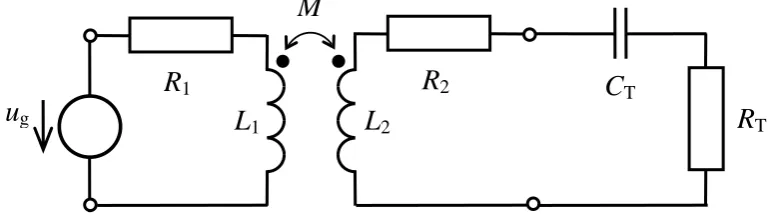
The original simplified model of circuit (Figure 1) includes loop antenna – represented by inductance L2,

transmitting antenna that is placed on passing vehicle – represented by inductance L1, and their inductive

coupling M when the vehicle passes through. The antenna is tuned on required operating frequency by capacitor

CT. Resistance RT is representing the circuit of a receiver.

u

R

L

L

M

R

C

R

C

II.

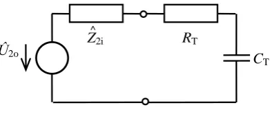
Following Thévenin´s theorem, the circuit from Fig. 1 can be replaced with loop antenna circuit from Fig. 2, where substitute impedance of the circuit is defined.

,

(1)

However, with respect to modelling circuit in MICRO-CAP system, we stuck to the circuit from figure 1.

Û2o

Z2i RT

CT

^

Fig. 2 Substitute scheme of loop antenna circuit

After the cable is included into antenna circuit, the scheme from figure 1 changes to scheme from figure 3. The cable is modelled by a T cell in two-port.

ug

R1

L1

L2

M

R2

CT

RT

CT

R0 dx L0 dx

G0 dx C0 dx

Fig. 3 Circuit model after cable inclusion

Concerning the fact, that the permeable frequency of given cable is 10 times higher than the resonant frequency of the loop antenna, we can replace the cable with spatially distributed parameters from Figure. 3 with its own parameters that are lumped with a T cell in our case (figure 4). For the parameters of T cell, the following is valid:

, , , (2)

We are not taking into consideration the lead of the cable which is not stated by its manufacturer. The length of the cable is 40m.

R

L

R

L

C

Fig. 4 Substituting the cable with a T cell

    

  

    

 ₂

1 2 2 1

1 2 2 2 2

1 2 2 1

1 2 2 2

2i j

ˆ

L R

L M L

L R

R M R

Z

    

2 o C/2

l R

R  

2 o C/2

l L

L   _{C C l}

III.

If there is a case, when the circuit is not modelled in the MICRO-CAP system, it would be possible to simplify the model of the cable considering the chosen resonant frequency and values of longitudinal parameters of the cable only with its transverse capacity CC, which would be connected in parallel to the capacitor with CT

value on Figure 1. Consequently, the increase in resulting capacity then lowers the resonant frequency of the loop antenna circuit.

Two options of optimization the resonant frequency were considered – using a serial capacitor or a parallel inductor with the condition that the RT and CT parameters of original circuit from Figure 1 must be preserved.

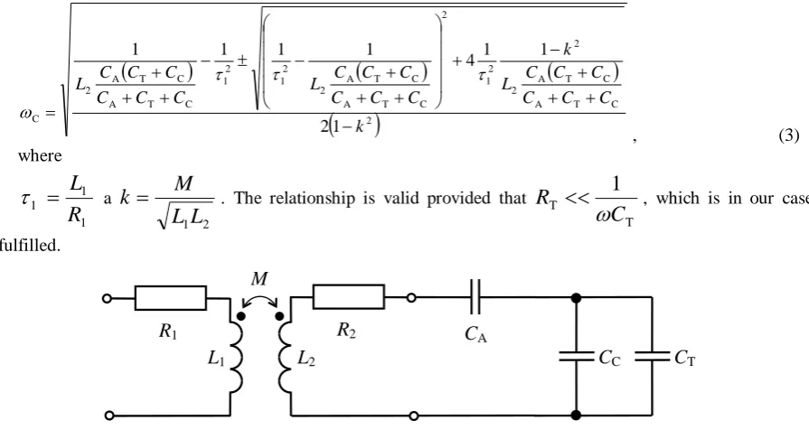
For the design of tuning parameters, the optimizing module of MICRO-CAP system was used. Maximizing the voltage on the cable output, that occurs when the output current of the cable has maximum value, was necessary. Simplified substitute circuit with tuning capacity is shown on figure 5. Estimation of angular frequency when there is a maximal current after inclusion of serial capacity CA is done by following:

, (3)

where 1 1 1

R

L





2 1

L

L

M

k



T T

1

C

R





fulfilled.

ui

R1

L1 L2

M

R2

CT CC

CA

Fig. 5 Simplified substitute circuit with tuning capacity

A simplified substitute circuit with tuning inductance is shown on Figure 6. Estimation of angular frequency when there is a maximal current after inclusion of parallel inductance LA is done by following:

























T C 2 A A 2 2 1 2 2 2 1 T C 2 2 A A 2 2 1 T C 2 2 A A 2 L 1 2 1 4 1 1 1 1 1 k C C L L L L k C C k L L L L C C k L L L L                         



.

(4)

ui

R1

L1 L2

M R2 CT CC LA Q

Fig. 6 Simplified substitute circuit with tuning inductance

It is obvious from the relationships (3) and (4) that the frequency value is influenced, among others, by time constant of transmitting antenna 1 and a coupling coefficient k. The coupling coefficient is very small with

antennas, so that we can assume, that its influence on relationships described at (3) and (4) is practically none. If

















of the time constant has inverted values. Therefore, the elements where the square is present are not valid and for both frequencies the following can be stated:





C T A

C T A 2 C

π 2

1

C C C

C C C L f

 





and





2 A

A 2 L

π 2

1

C C L L

L L f

 



.

(5)

The above mentioned relationships apply for simplified conditions. If all parameters of the model are taken precisely, the analytic relationships would be excessively complicated and can be confusing. That is why the only option is to use simulating software such as MICRO-CAP.

IV.

Simulations in MICRO CAP system were carried out for following parameters: ugp-p = 2V, R1 = 122 , L1 =

678 H, R2 = 2 , L1 = 806 H, M = 16 H, RT = 54 , CT = 2.2 nF, RC/2 = 780 m, LC/2 = 13 H, CC = 6 nF.

The value of tuning capacity which was calculated by optimizing module of MICRO-CAP system is CA = 2,9

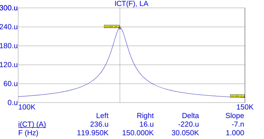
nF after rounding. The value of tuning inductance is LA = 268 H. Appropriate frequency characteristics of

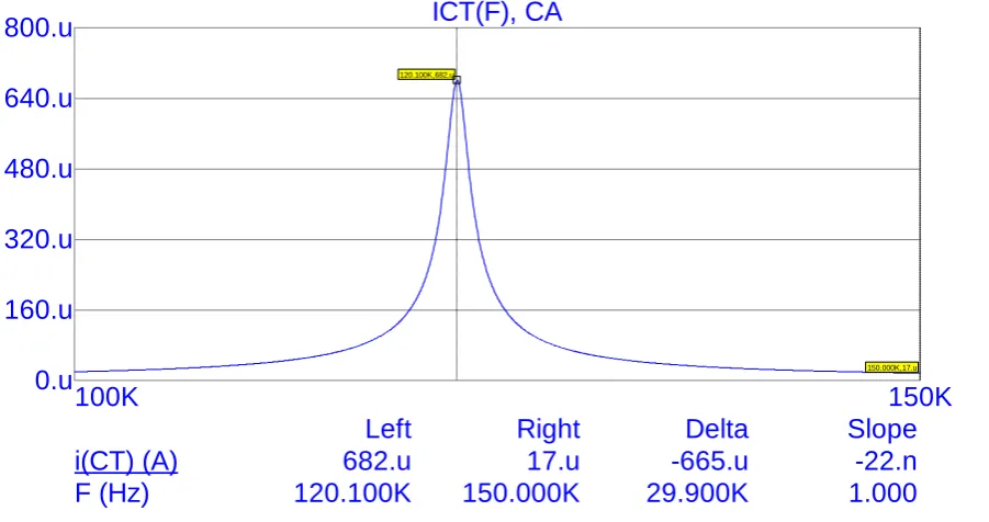
output current are shown on figures 6 and 7. From the pictures, it is obvious, that it is more suitable to use tuning capacity, because the maximal current output is approx. 3 times higher.

Fig. 6 Frequency characteristics of output current of the cable, CA = 2,9 nF

100K

150K

0.u

160.u

320.u

480.u

640.u

800.u

i(CT) (A)

F (Hz)

ICT(F), CA

Left

Right

Delta

Slope

150.000K,17.u 120.100K,682.u

682.u

17.u

-665.u

-22.n

Fig. 7 Frequency characteristics of output current of the cable, LA = 268 H

V.

In conclusion we can say that even the MICRO-CAP system has its limitations and problems when modelling the cables with the use of TLine model. Those limitations can be avoided using the cascading of T or  cells according to desired frequency range. It was satisfying to use only one T cell for modelling in our case because the permeable frequency of the cable has the value of approximately 1.2 MHz. Optimizing module of the MICRO CAP system enables to easily find the value of desired parameters, that are in our case the tuning capacity CA and the inductance LA; so that the antenna is tuned on desired frequency of 120 kHz even after

using the cable. From the simulation of these two circuits, it can be stated that it is more appropriate to use the tuning capacity than tuning inductance, which ensures higher value of output voltage of the cable

ACKNOWLEDGEMENT

This research is supported by the project SP2016/143 “Research of antenna systems; effectiveness and diagnostics of electric drives with harmonic power; reliability of the supply of electric traction; issue data anomalies.”. The authors would like to express their thanks to the members of Department of Electrical Engineering at VSB – Technical University of Ostrava for their valuable instructions and support.

R

EFERENCES

[1] M.Mikulec and V.Havlicek, Basic circuit theory, Vydavatelstvi CVUT, Prag, 2005, ISBN 80-01-03172-1. [2] Micro-Cap 8.0 Electronic Circuit Analysis Program, User’s Guide, 2004.

[3] Micro-Cap 8.0 Electronic Circuit Analysis Program, Reference manual, 2004.

100K

150K

0.u

60.u

120.u

180.u

240.u

300.u

300.u

i(CT) (A)

F (Hz)

ICT(F), LA

Left

Right

Delta

Slope

150.000K,16.u 119.950K,236.u

236.u

16.u

-220.u

-7.n