Maximum Likelihood Method and Cramer-Rao Low Bound of Angle
Estimation for Wide-Band Monopulse Radar
Haibo Wang*, Wenhua Huang, Yue Jiang, and Tao Ba
Abstract—The echo signal of wide-band monopulse radar spreads in multiple range cells. Thus, effective utilization of echo signal is an important issue for this kind of radar. Based on parameter estimation model, maximum likelihood method is proposed in this paper, which collects all the energy spreading in multiple range cells. Cramer-Rao low bound of angle estimation is deduced in theory. Simulation results demonstrate maximum likelihood method which performs better than both dominant scatter estimate method and weighted estimate method.
1. INTRODUCTION
Monopulse is a simultaneous lobbing technique for precisely determining the angle of arrival of echo signal, which is adopted for narrow-band radars. Under the condition that there is only a single point target in a given range cell, estimation of the direction of arrival (DOA) of target is easy to be understood [1–3]. Maximum likelihood solution for the angle estimation is obtainable [4] by monopulse complex ratio, and its accuracy is close to Cramer-Rao Low bound (CRLB) asymptotically under the circumstance of moderate or high signal-to-noise ratio (SNR). Several efficient approaches to extraction from standard monopulse signals and the angles of unresolved targets have been proposed [5–7]. Wang et al. [8] discussed DOA estimation of two unresolved Rayleigh targets based on monopulse measurements and presented maximum likelihood solution in that scenario.
Nowadays, wide-band radars are more and more prevalent. Range cell of a wide-band radar is much smaller than conventional narrow-band radars. Thus, single point target model is not suitable for description of echo signal of wide-band radars any more. In other words, the target echo may occupy multiple range cells, commonly. Howard [9] reported the experiment result of a high range resolution monopulse tracking radar and drew a conclusion that detailed information of target and reduction of angle scintillation can be provided by high range resolution monopulse tracking radar. Due to the high range resolution of wide-band radar, echo form target always spreads into multiple range cells. Therefore, the challenge of angle estimation for wide-band monopulse radar lies in how to accumulate energy of target echo form high resolution range profiles (HRRP). Zhang et al. [10] proposed a estimation method for linear frequency modulated (LFM) radar, in which angle estimation is translated to estimate the frequency of cross-correlation function (CCF). The frequency of the main spectral line can be estimated by fast Fourier transform (FFT) or other frequency estimation methods. However, CCF method is not suitable for other types of band modulated signal. Chen [11] proposed a signal model for wide-band resolution monopulse radar, and the maximum likelihood angle estimation method is proposed based on numerical solution for nonlinear equations with iterative algorithm, which consumes many computational resources.
Received 25 April 2018, Accepted 6 July 2018, Scheduled 24 July 2018 * Corresponding author: Haibo Wang ([email protected]).
In this paper, with series of mathematical derivations, we find that close-form maximum likelihood method of angle estimation for wide-band monopulse radar does exist, regardless of wide-band modulation method. CRLB of angle estimation is deduced, which reveals that collecting all of energy spreading in multiple range cells could get better angle estimation result.
The remaining of this paper is organized as follows. Problem description and signal model of monopulse angle estimation are presented in Section 2. The proposed maximum likelihood method and CRLB of angle estimation are introduced in Section 3 and Section 4, respectively. In Section 5, we present the comparison of angle estimation results calculated by proposed method and other estimation methods. Finally, we give some conclusions in the last section.
2. PROBLEM DESCRIPTION AND SIGNAL MODEL
2.1. Monopulse Phase Comparisons Angle Estimation
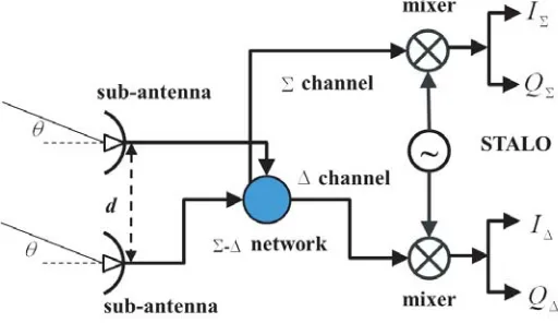
Before we introduce the proposed method, the principle of classical monopulse angle estimation is discussed briefly in this section. Fig. 1 depicts the receiver configuration of monopulse angle estimate radar. The phase centers of two identical antennas are located in the system with baseline d. Radio frequency(RF) signals from two antennas feed into a Σ-Δ network. Signals in Σ-channel and Δ-channel are down-converted by stabilized local oscillator (STALO) in radar receiver, and HRRPΣ and HRRPΔ
are generated by matched filter respectively.
Figure 1. Receiver configuration of monopulse angle estimate radar.
Two antennas, with separate phase centers, have identical far-field distributionsF(θ). Theirs axes are parallel to each other, and it is also the axis of the whole radar system. Assume that the target echo signal comes from angle θ, which means angle error to antennas system axis. Then output of complex amplitude in Σ-channel and Δ-channel can be described as
FΣ(θ) =
√ 2 2 F(θ)
exp
j2π
λ sin(θ) d
2
+ exp
−j2π
λ sin(θ) d
2
=√2F(θ) cos
πdsin(θ)
λ
(1)
FΔ(θ) =
√ 2 2 F(θ)
exp
j2π
λ sin(θ) d
2
−exp
−j2π
λ sin(θ) d
2
=√2jF(θ) sin
πdsin(θ)
λ
(2)
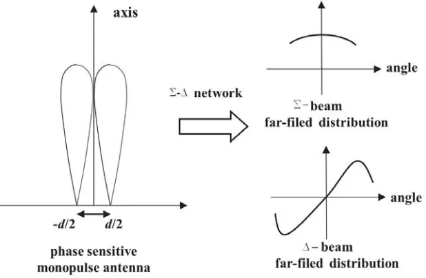
where λ is the carrier wavelength. Eq. (1) and Eq. (2) are also entitled as Σ-beam and Δ-beam, respectively, for the whole antenna system. Σ-beam and Δ-beam are displayed in Fig. 2.
The complex amplitude ratio between Σ-beam and Δ-beam is
FΔ(θ)
FΣ(θ)
= jf(θ) = j tan
πdsin(θ)
λ
≈jπd
λ θ (3)
Figure 2. Σ-beam and Δ-beam.
is usually employed in practice, which is named as angle estimation S-curve. According to S-cure, angle estimation can be obtained from complex amplitude ratio between Σ-channel and Δ-channel.
2.2. Signal Model of Angle Estimation in Wideband Monopulse Radar
Wide-band radar transmits wide-band waveforms, such as direct short pulse [9, 12], phase coding pulse, and linear frequency modulation (LFM) pulse. For all kinds of wide-band waveforms, HRRP can be obtained by matched filter, in other words, pulse compress. Without loss of generality, direct short pulse is used as an example to deduce the algorithm in this paper.
Consider a range extending target spreading its echo in N range cells, which has a different amplitude and phase in each range cell. It is located in the far-field of radar system, so that the angular glint from different scatter centers is negligible. Assuming that target is located in angle θ
according to radar axis, consequently signals in Σ-channel and Δ-channel can be written as
xΣ(n) =s(n) +w1(n)
xΔ(n) = jf(θ)s(n) +w2(n)
(4)
where n denotes the range cells index number, n = 0,1,2, . . . , N −1. s(n) is the HRRP of target.
w1(n) and w2(n) are receiver noises in Σ-channel and Δ-channel. We assume that w1(n) and w2(n)
are zero-means complex white Gaussian random processes, correspondingly w1(n), w2(n)∼CN(0, σ2),
which are also independent from each other in different range cells. In order to be concise, Eq. (4) is rewritten in a vector form
xΣ =s+w1
xΔ= jf(θ)s+w2
(5)
where xΣ, xΔ and s are Σ-channel vector, Δ-channel vector and HRRP of target vector. w1 and w2
are noise vectors in Σ-channel and Δ-channel, respectively. The ultimate goal of angle estimation is to use the measured data, namely xΣ and xΔ, to calculate angle of target, that is θ.
Dominant scatter method is very easy to implement, as to range extending target, which can be expressed by the formula:
ˆ
θ=f−1xΣ(m) xΔ(m)
≈ λ
πd
xΣ(m)
xΔ(m)
, m= argmax
n
It is obvious that the echo energy of scatter is unusable except the dominant scatter. Weighted method is also used:
ˆ
θc = K−1
k=0
ωkθk, subject to : K−1
k=0
ωk= 1, ωk≥0 (7)
in whichK denotes the number of scatter centers that can be found by the target detection algorithm, andθkcan be calculated by Eq. (6) with the range cell index correspondingly. ωkrepresents the weights
of each scatter center. Conventionally, equivalent weights are easy to implement for the real world applications.
3. MAXIMUM LIKELIHOOD ESTIMATION
In order to obtain the theoretical derivation of maximum likelihood estimation, parameter transform is employed:
α=f(θ), θ=f−1(α) (8) where the parameter α is a real number. The likelihood functions of Σ-channel and Δ-channel can be expressed as follow:
PΣ(xΣ|s) =
1
πNσ2N exp
− 1
σ2(xΣ−s) H(x
Σ−s)
PΔ(xΔ|s, θ) =
1
πNσ2N exp
− 1
σ2(xΔ−jαs) H(x
Δ−jαs)
(9)
where ()H denotes the conjugate transpose operator. Then log-likelihood function of all data vectors can be written as
logP(xΣ,xΔ|s, α) = −
1
σ2
xHΣxΣ+xHΔxΔ−
xHΣs+sHxΣ
−jαxHΔs−sHxΔ
+1 +α2sHs) −2Nlog(πσ2) (10)
We further examine the partial derivatives of Eq. (10) and obtain the equations forα and s
∂logP(xΣ,xΔ|s, α)
∂α = −
1
σ2
−jxHΔs−sHxΔ
+ 2αsHs = 0 (11)
∂logP(xΣ,xΔ|s, α)
∂s = − 1
σ2
−x∗Σ−jαx∗Δ+1 +α2s∗ =0 (12)
where ()∗ means conjugate operator. The solution of Eq. (11) and Eq. (12) is maximum likelihood estimation of α. Consequently, maximum likelihood estimation ofθ can be expressed as
ˆ
αMLE= j
xH
ΣxΔ−xHΔxΣ
2xHΣxΣ ,
ˆ
θMLE=f−1( ˆαMLE) (13)
The details can be found in Appendix A.
4. CRAMER-RAO LOW BOUND
To study the performance of parameter estimation, Fisher Information Matrix (FIM) is deduced. Consequently, the close form of CRLB is obtained
J(α,s) = −E
⎡ ⎢ ⎢ ⎣
∂2logP(xΣ,xΔ|s, α)
∂α2
∂2logP(xΣ,xΔ|s, α)
∂α∂s
T
∂2logP(xΣ,xΔ|s, α)
∂s∗∂α
∂2logP(xΣ,xΔ|s, α)
∂s∗∂s
⎤ ⎥ ⎥ ⎦ (14) = 1 σ2
sHs αsH
αs (1 +α2)IN×N
By inverse of FIM, CRLB of α can be written as
var( ˆα)≥J−1(α,s)11= (1 +α2) σ 2
sHs =
1 +α2
SNRCA
(16)
where SNRCA is defined as coherent accumulating echo signal to noise ratio for the range extending
target, which means that the whole target echo energy spreading in range cells is collected exactly. It is quite different from the signal to noise ratio of a single point target. Therefore, the essence of angle maximum likelihood estimation in Eq. (13) is that all the scatters distributed in multiple range cells provide their contributions to angle estimation. More details can be found in Appendix B.
The CRLB ofθ is
var(ˆθ) ≥
∂θ ∂α
2
J−1(α,s)11=
1 + (f(θ))2
∂f ∂θ
2 σ
2
sHs (17)
≈
λ πd
2
+θ2
σ2
sHs ≈
λ πd
2 1
SNRCA
(18)
where the approximate conditions is θ πdλ. Based on the result of CRLB in this section, estimation accuracy curves under typical conditions can be plotted. Fig. 3 plots the standard deviation of angle estimation error under different phase center distances and different target angles. From Fig. 3, the conclusion can be made as follows
(i) Target angle has a little influence on CRLB of angle estimation. Only a little difference can be observed under the condition ofd= 20λ.
(ii) A longer baseline promotes better angle estimation results. However, it means larger aperture antenna, commonly.
(iii) High SNRCA guarantees good performance of angle estimation.
5 10 15 20 25 30
10-2 10-1 100 101
SNRCA (dB)
sqrt of CRLB (deg)
d = 10 λ ,θ = 0.1 deg d = 10 λ ,θ = 0.3 deg d = 20 λ , θ = 0.1 deg d = 20 λ ,θ = 0.3 deg
Figure 3. CRLB (θ) against SNRCA.
5. SIMULATION RESULTS
In this section, simulations are conducted to demonstrate the effectiveness and feasibility of the algorithm. The detail of simulation setup is as follows.
-2 -1 0 1 2 -1
-0.5 0 0.5 1 1.5 2
θ / θ3dB
amplitude
Σ channel
Δ channel
-2 -1 0 1 2 -2
-1.5 -1 -0.5 0 0.5 1 1.5 2
θ / θ3dB
Δ
channel
/
Σ
channel
S curve
linear approximation
(a) (b)
Figure 4. Σ-channel and Δ-beam of antenna. (a) Relative amplitude of Σ-channel and Δ-channel against target angle. (b) S-curve and its linear approximation.
Σ-channel and Δ-channel against target angle are shown in Fig. 4(a). Therefore, S-curve and its linear approximation can be obtained, which is illustrated in Fig. 4(b).
The wide-band radar transmits short pulse with pulse width τ = 10 ns; therefore, the range resolution is 1.5 m. The spectrum spread is 100 MHz by the pulse modulation. The carrier frequency is fc = 10 GHz. RF signals of both the Σ-channel and Δ-channel are obtained by time-domain
reconstruction. To simulate signal flow in a wide-band monopulse radar system, a digital orthogonal mixer, digital filters and data resampling are utilized to down convert RF signal to the baseband, for the implementation of algorithms. The sampling rate of IF signal is 200 MHz in both I-channel and Q-channel.
5.1. Simulation of the Multiple Point Scatters Target
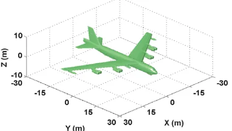
Suppose that there is a target containing 13 scattering centers with equivalent weights. The target is located in the far-field of radar antenna. Thus, the angle glint effect is neglected. The target angle is 0.3 degree versus the axis of antenna. Geometry of both antennas of wide-band radar and scattering centers of target are illustrated in Fig. 5. The echo signal can be obtained by the following equation
x(t) =
m
Ams
t−2(rm−rref) c
(19)
where m is the index of scattering centers, m = 1,2, . . . ,13. Am is the reflective ratio for each center
respectively, and the ratios are set to be equal, in this scenario. rm is the range of each scattering
center from radar coordinate. The projection of scattering centers onto the radar line of sight can be used to calculate rm, which is illustrated by Fig. 5. rref is the reference range for simulation, and s(t)
is thetransmitting signal of radar.
Figure 6 displays the RF signals of both Σ-channel and Δ-channel. It is obvious to find that there are 6 echoes in range profile other than 13 centers in simulation setup displayed in Fig. 5. Some of the scattering centers are located near each other, thus they cannot be resolved by the transmitting signal of radar, in other words, staying in the same range cell. The magnitudes of 6 echoes in the range profile in Fig. 6 are different from each other.
sHs is calculated manually before adding noise. The noise is generated with given SNRCA. In this
simulation, the gap between SNRCA and SNRPEAK can be evaluated
Figure 5. Geometry of both antenna of wide-band radar system and target.
0 50 100 150 200 250 -20
0 20
time (ns)
amplitude
RF signal in Σ channel
0 50 100 150 200 250 -2
0 2
time (ns)
amplitude
RF signal in Δ channel
Figure 6. RF signal of both the Σ-channel and Δ-channel.
where SNRPEAK denotes the signal to noise ratio of the dominant scatter. The method to obtain
Eq. (20) is to treat 6 echoes in Fig. 6 as single point scatter. Consequently, target angle is estimated by dominant scatter estimate method, weighted estimate method and maximum likelihood method, respectively. Equivalent weights are set up in Eq. (7).
Monte-Carlo method is employed to obtain the root mean square error (RMSE) of angle estimation, in which the simulation is repeated over 10,000 times. Fig. 7 illustrates RMSE result and CRLB under the given SNRCA. It can be found that RMSE of maximum likelihood method is much smaller than
both dominant scatter estimate method and weighted estimate method. With the increase of SNRCA,
RMSE of maximum likelihood method trends to CRLB, asymptotically.
5.2. Electromagnetic Simulation of Range Extend Target
22 24 26 28 30 32 34 36 38 40 10-2
10-1 100
SNRCA (dB)
sqrt of CRLB or RMSE (deg)
sqrt of CRLB
donimant scatter estimate weighted estimate
maximun likelihood estimate
Figure 7. RMSE and CRLB (target with 13 scattering centers).
Figure 8. Shape and imaging geometry of airplane.
time and memory. Thus, we use the PO method to calculate wide-band scatter characteristics of the target, which reserves the advantage of fast computing speed and low memory demand. Time domain echo signal of the target can be rebuilt by wide-band scatter characteristics as follows.
x(t) = 1
πRe
f0+B/2
f0−B/2
H(f) exp(2πjf t)df
∗s(t) (21)
where s(t) is the wide-band signal transmit by radar, with the carrier frequencyf0. H(f) is the
wide-band scatter characteristics of the target, including the amplitude and phase information. B is the bandwidth of PO calculation, the center of which is f0. x(t) is the time domain echo signal of target.
‘∗’ denotes the convolution operator. Then, Fig. 9 displays the waveform and its envelope of microwave short pulse echo, which is quite different from the incident pulse waveform. The gap between SNRCA
and SNRPEAK is not easy to obtain, in this scenario.
Monte-Carlo method is also employed to obtain the RMSE of angle estimation, with 10,000 times repetition. Fig. 10 illustrates RMSE result and CRLB under the given SNRCA. It can also be found that
0 50 100 150 200 250 -0.2
-0.15 -0.1 -0.05 0 0.05 0.1 0.15 0.2
time (ns)
normalized scattered field (V)
waveform envelope
Figure 9. Waveform and its envelop of echo signal.
22 24 26 28 30 32 34 36 38 40 10-2
10-1 100
SNRCA (dB)
sqrt of CRLB or RMSE (deg)
sqrt of CRLB
donimant scatter estimate weighted estimate
maximun likelihood estimate
Figure 10. RMSE and CRLB (airplane).
6. CONCLUSIONS
This paper focuses on angle estimation method for wide-band monopulse radar. In order to use echo signal energy effectively, we propose a maximum likelihood method for angle estimation of the target whose echo spreads in multiple range cells. Close form of CRLB is obtained, which suggests that coherent accumulation echo signal in range cells should be employed in estimation method. Simulation results verify the proposed method, and comparison of three kinds of estimation method shows that maximum likelihood method performs the best.
Angle glint effect has not been considered in the signal model. The mechanics of angle glint lie on the electromagnetic scatter in the near-field region of the radar. In theory, the information of angle collecting for multiple range cells should be much more creditable. Thus, angle glint suppression effect by the proposed method for wide-band monopulse radar will be researched in future work.
APPENDIX A. DERIVATION OF THE EQUATIONS OF α AND S
According to the log-likelihood function given in Eq. (10), the derivative log-likelihood function can be obtained directly. The rules of derivatives of complex vector are listed as follow [15]
∂yHx
∂x =y
∗, ∂xHy
∂x =0
∂xHAx
∂x = (Ax)
∗, ∂xHx
∂x =x
∗
(A1)
where A is the Hermite matrix, namely AH =A. According to the rules in Eq. (A1), the derivative log-likelihood function is inferable as Eq. (12). Thus,s can be written as
s= 1
1 +α2(xΣ−jαxΔ) (A2)
Substitution of Eq. (A2) into Eq. (11) and simplification gives an equation in terms ofα
Aα2+Bα+C= 0 (A3)
where,
A= jxHΔxΣ−xHΣxΔ
, B= 2xHΣxΣ−xHΔxΔ
, C=−jxHΔxΣ−xHΣxΔ
α is a real number, and solutions of quadratic Eq. (A3)
α= −B± √
B2−4AC
2A (A5)
With simplification of Eq. (A5), we have
α1 = j
xHΣxΔ−xHΔxΣ
2xH ΣxΣ
, α2= j
2xHΣxΣ
xH
ΣxΔ−xHΔxΣ
(A6)
α2 is unreasonable, which is ignored. Then maximum likelihood estimation ofαandθcan be expressed
as
ˆ
αMLE= j
xHΣxΔ−xHΔxΣ
2xHΣxΣ ,
ˆ
θMLE =f−1( ˆαMLE) (A7)
It is very easy to find that ˆαMLE is a real number indeed,
( ˆαMLE)∗= (−j)
xH ΣxΔ
∗
−xH ΔxΣ
∗
2xH ΣxΣ
∗ = ˆαMLE (A8)
APPENDIX B. DERIVATION OF CRLB OF α
Lemma of block matrix inverse. Consider a matrixA:
A=
A11 A12
A21 A22
=
k×k k×(n−k) (n−k)×k (n−k)×(n−k)
(B1)
Suppose that A11 and A22 are nonsingular, then
A−1=
A11−
A12A−221A21
−1
−A11−A12A−221A21
−1
A12A−221
−A22− −A21A−111A12
−1
A21A−111 A22−
A21A−111A12
−1
(B2)
Eq. (14) draws as follows:
var( ˆα)≥J−1(α,s)11=σ2
sHs−αsH 1
1 +α2IN×Nαs
−1
= 1
1 +α2
σ2
sHs (B3)
REFERENCES
1. Mosca, E., “Angle estimation in amplitude comparison monopulse systems,” IEEE Transactions on Aerospace and Electronic Systems, Vol. 5, No. 4, 205–212, 1969.
2. Hofstetter, E. M. and D. Delong, “Detection and parameter estimation in an amplitude-comparison monopulse radar,”IEEE Transactions on Information Theory, Vol. 15, No. 1, 22–30,1969.
3. Nickel, U., “Overview of generalized monopulse estimation,” IEEE Aerospace and Electronic Systems Magazine, Vol. 21, No. 6, 27–56, 2006.
4. Blair, W. D. and M. Brandt-Pearce, “Statistical description of monopulse parameters for tracking rayleigh targets,” IEEE Transactions on Aerospace and Electronic Systems, Vol. 34, No. 2, 597– 611,1997.
5. Blair, W. D. and M. Brandt-Pearce, “Monopulse doa estimation of two unresolved rayleigh targets,”
IEEE Transactions on Aerospace and Electronic Systems, Vol. 37, No. 2, 452–469, 2002.
6. Berkowitz, R. and S. Sherman, “Information derivable from monopulse radar measurements of two unresolved targets,” IEEE Transactions on Aerospace and Electronic Systems, Vol. 7, No. 5, 1011–1019, 2007.
8. Wang, Z., A. Sinha, P. Willett, and Y. Bar-Shalom, “Angle estimation for two unresolved targets with monopulse radar,” IEEE Transactions on Aerospace and Electronic Systems, Vol. 40, No. 3, 998–1019, 2004.
9. Howard, D. D., “High range-resolution monopulse tracking radar,”IEEE Transactions on Aerospace and Electronic Systems, Vol. 11, No. 5, 749–755, 1975.
10. Zhang, Y. X., Q. F. Liu, R. J. Hong, P. P. Pan, and Z. M. Deng, “A novel monopulse angle estimation method for wideband lfm radars,” Sensors, Vol. 16, No. 6, 817–825, 2016.
11. Chen, X. L., “An angle measurement method for high resolution radar based on maximum likelihood estimation,”Signal Processing, Vol. 16, No. 6, 817–625, 2012 (in Chinese).
12. Blyakhman, A., D. Clunie, R. Harris, and G. Mesyats, “Nanosecond gigawatt radar: Indication of small targets moving among heavy clutters,”Radar Conference, 61–64, 2007.
13. Asvestas, J. S., “The physical-optics integral and computer graphics,” IEEE Transactions on Antennas and Propagation, Vol. 43, No. 12, 1459–1460, 1995.
14. Uiku, H. K. and A. A. Ergin, “Radon transform interpretation of the physical optics integral and application to near and far field acoustic scattering problems,” IEEE Antennas and Propagation Society International Symposium, 1–4, 2010.