Scholarship@Western
Scholarship@Western
Electronic Thesis and Dissertation Repository
9-24-2019 3:30 PM
Finite Element Analysis of Hollow-stemmed Shoulder Implants in
Finite Element Analysis of Hollow-stemmed Shoulder Implants in
Different Bone Qualities Derived from a Statistical Shape and
Different Bone Qualities Derived from a Statistical Shape and
Density Model
Density Model
Pendar Soltanmohammadi
The University of Western Ontario
Supervisor Willing, Ryan T.
The University of Western Ontario
Graduate Program in Biomedical Engineering
A thesis submitted in partial fulfillment of the requirements for the degree in Master of Engineering Science
© Pendar Soltanmohammadi 2019
Follow this and additional works at: https://ir.lib.uwo.ca/etd
Part of the Biomedical Engineering and Bioengineering Commons
Recommended Citation Recommended Citation
Soltanmohammadi, Pendar, "Finite Element Analysis of Hollow-stemmed Shoulder Implants in Different Bone Qualities Derived from a Statistical Shape and Density Model" (2019). Electronic Thesis and Dissertation Repository. 6631.
https://ir.lib.uwo.ca/etd/6631
This Dissertation/Thesis is brought to you for free and open access by Scholarship@Western. It has been accepted for inclusion in Electronic Thesis and Dissertation Repository by an authorized administrator of
ii
The incidence of total shoulder arthroplasty procedures (TSA) to treat osteoarthritis has
experienced the most rapid growth among all human joint replacements. However, stress
shielding of proximal bone following its reconstruction is a complication of TSA triggering
unfavorable adaptive bone remodeling, especially for osteoporotic patients.
A better understanding of how the shape and density of the shoulder vary among members of
a population can help design more effective population-based orthopedic implants. Therefore,
finite element models representing healthy, osteopenic, and osteoporotic bone qualities in a
population were developed using our statistical shape and density model. Bones were
reconstructed with hollow- and solid-stemmed implants and resulting changes in bone stresses
were calculated. We concluded that the use of more compliant stems, such as hollow stems,
could marginally mitigate the effect of stress shielding at the proximal humerus. Further
increasing the compliance of stems by making them porous could improve bone-implant
mechanics.
Keywords
Shoulder, Osteoarthritis, Total shoulder arthroplasty, Stress shielding, Osteoporosis, Bone
mechanics, Implant design, Finite element analysis, Statistical shape model, Statistical density
iii
Summary for Lay Audience
Osteoarthritis of the shoulder is a joint disease that can result in severe pain and stiffness. Total
shoulder arthroplasty (TSA) is a clinically successful surgery to relieve pain and restore the
natural range of motion to the arthritic shoulder joint. The number of patients who undergo
TSA has experienced rapid growth, more than any other joint in the human body over the past
decades and is continuing to grow. A seven-fold increase in its incidence is predicted for the
next decade. During TSA, an implant is inserted into the humerus bone, the bone of the upper
arm, to reconstruct the shoulder joint. However, due to altered loading transmission following
implantation, the proximal (near the upper end) humerus will be shielded from experiencing
stress. Bone is a self-optimizing structure, which means that it adapts its structure according to
the exerted loads. Therefore, the reduction of stress in the proximal humerus can lead to bone
loss, implant loosening and, finally, a need for revision surgery.
Humeral implants are comprised of two sections, namely, the stem component and the head
component. The design of humeral implants and specifically their stem component has a
significant influence on the overall implant success, as the stem is responsible for load transfer
from the head component of the implant to the surrounding bone.
We found that the use of more compliant shoulder implants with hollow stems could
marginally mitigate the effect of stress shielding and consequently reduce the need for revision
surgeries of the shoulder. Also, an exacerbation of stress shielding was found for patients
suffering from osteoporosis, a bone disease in which deterioration of bone tissue occurs. Our
study suggests that further increasing the compliance of implant stems by making them also
porous could increase the bone stresses at the proximal humerus and, therefore, further limit
iv
Co-Authorship Statement
Chapter 1:
Pendar Soltanmohammadi – Performed the literature survey, helped craft project objectives and wrote the manuscript.
Ryan Willing – Edited the manuscript.
Chapter 2:
Pendar Soltanmohammadi – Developed models, performed data analysis and wrote the manuscript.
Vishnu Veeraraghavan and Josie Elwell – Segmented the CT images and generated surface geometries with identical mesh topologies and edited the manuscript.
Derek Jacobs – Assigned nodal density properties to each specimen’s volume mesh with an automated code provided by Pendar Soltanmohammadi.
Ryan Willing – Edited the manuscript.
Chapter 3:
Pendar Soltanmohammadi – Developed models, performed data analysis and wrote the manuscript.
Derek Jacobs – Segmented the healthy and osteoporotic CT images. George Athwal – Supervised the positioning of the implant
Ryan Willing – Edited the manuscript.
Chapter 4:
v
Acknowledgments
I would like to thank my supervisor, Dr. Ryan Willing, for his illuminating guidance and
enduring inspiration throughout this research project. Also, I take this opportunity to thank my
advisory committee members, Dr. Athwal and Dr. Lalone, for their helpful instructions. I
appreciate the support of my fellow labmates at the Musculoskeletal Biomechanics Laboratory
at Western University. I am also grateful to Derek Jacobs for his assistance in this project.
This work would not have been possible without the never-ending support of my family and
friends: Mehdi Soltan Mohammadi, Samaneh Zaferani, Alireza Rezazadeh, Jahanbakhsh
Jahanzamin, Alireza Moslemian, Alisaleh Shariati, Amir Tavakoli, Armin Geraili, and Geofrey
Yamomo.
Although words are not capable of expressing my eternal debt of gratitude to my beloved
parents and my dear sister, I will take this opportunity to dedicate this thesis to them who have
vi
Table of Contents
Abstract ... ii
Summary for Lay Audience ... iii
Co-Authorship Statement... iv
Acknowledgments... v
Table of Contents ... vi
List of Tables ... viii
List of Figures ... ix
List of Appendices ... xi
Chapter 1 ... 1
1 Introduction ... 1
1.1 Anatomy of the Shoulder ... 2
1.1.1 Osseous Constructs ... 3
1.1.2 Soft Tissue Constructs ... 6
1.2 Structure and Material Properties of Shoulder Bones... 7
1.2.1 Structure of Bone ... 7
1.2.2 Material Properties of Bone ... 8
1.3 Shoulder Arthroplasty ... 9
1.4 Wolff’s Law and Stress Shielding ... 12
1.5 Statistical Shape and Density Modeling ... 14
1.6 Finite Element Simulation of Shoulder Arthroplasty ... 16
1.7 Project Scope and Objectives ... 17
1.8 Thesis Overview ... 18
Chapter 2 ... 19
vii
2.1 Introduction ... 19
2.2 Methods... 21
2.2.1 Development of Statistical Shape and Density Models ... 21
2.2.2 Data Analysis ... 25
2.3 Results ... 26
2.4 Discussion ... 37
Chapter 3 ... 42
3 Structural Analysis of Hollow- Versus Solid-stemmed Shoulder Implants of Proximal Humeri with Different Bone Qualities ... 42
3.1 Introduction ... 42
3.2 Methods... 43
3.3 Results ... 52
3.4 Discussion ... 63
Chapter 4 ... 68
4 Summary and Future Works ... 68
4.1 Summary ... 68
4.2 Limitations and Strengths ... 69
4.3 Future Directions ... 71
4.4 Significance... 72
References ... 73
Appendices ... 86
viii
List of Tables
Table 2.1 The demographic data for male and female sub-groups ... 25
Table 3.1 Number of donors in each category of bone disease conditions along with the
cutoff HUs used for classifications ... 45
Table 3.2 Values of joint reaction forces (N) and frictional moments (N.mm) applied to the
ix
List of Figures
Figure 1.1 Three common planes used to define anatomy ... 2
Figure 1.2 Bones and articulations of the shoulder... 3
Figure 1.3 Bony Landmarks of the humerus ... 5
Figure 1.4 Bony landmarks of the scapula ... 6
Figure 1.5 The main forms of shoulder reconstruction ... 10
Figure 2.1 Steps taken toward developing SSMs from CT images ... 21
Figure 2.2 Baseline mesh mapping ... 22
Figure 2.3 The first two modes of shape variation of the shoulder ... 27
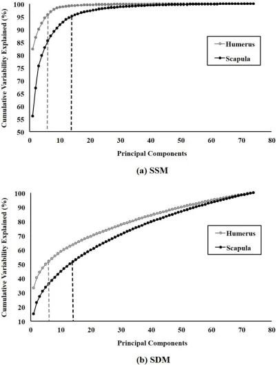
Figure 2.4 Cumulative sum of the variability percentage explained by the respective number of PCs ... 29
Figure 2.5 The shape of the humerus and scapula averaged over the entire population and averaged over male/female sub-group ... 30
Figure 2.6 The boxplot of the PC scores of male and female humeri in the well-matched set for shape ... 31
Figure 2.7 The boxplot of the PC scores of male and female scapulae in the well-matched set for shape ... 32
Figure 2.8 The boxplot of the PC scores of male and female humeri in the well-matched set for density ... 33
Figure 2.9 The Boxplot of the PC scores of male and female scapulae in the well-matched set for density ... 34
x
Figure 3.1 Defined slices to measure density in the proximal humerus ... 44
Figure 3.2 Solid- and hollow-stemmed implants ... 46
Figure 3.3 Mesh Planning ... 47
Figure 3.4 Humeral coordinate systems used for the right humeri along with the boundary
conditions applied to their distal end ... 50
Figure 3.5 Outcome measures were quantified regionally for chosen cortical and trabecular
bone slices ... 52
Figure 3.6 The volume-weighted average change in the magnitude of von Mises stress for the
reconstructed cortical bone ... 54
Figure 3.7 The volume-weighted average change in the magnitude of von Mises stress for the
reconstructed trabecular bone ... 55
Figure 3.8 The volume-weighted average deviatoric component of the change in stress tensor
for the reconstructed cortical bone ... 57
Figure 3.9 The volume-weighted average deviatoric component of the change in stress tensor
for the reconstructed trabecular bone ... 58
Figure 3.10 The percentage of cortical bone volume with the resorption/formation potential
for each bone condition and each stem design ... 60
Figure 3.11 The percentage of trabecular bone volume with the resorption/formation
xi
List of Appendices
Appendix A. Specimen Reconstruction Using a Compact SSM/SDM ... 86
Appendix B. SSM Robustness Analysis ... 88
Appendix C. SDM Robustness Analysis ... 90
Chapter 1
1
Introduction
Total shoulder arthroplasty (TSA) is widely regarded as a clinically successful surgery,
relieving pain, and restoring the natural range of motion (ROM) to an arthritic shoulder
joint [1]–[3]. It has the most rapid growth among all human joint replacement procedures,
with a projected seven-fold increase in its utilization over the next decade [4]. The number
of TSA and hemiarthroplasty procedures performed in the United States increased from
approximately 19,000 in 2000 [5] to more than 66,000 in 2011 [6]. The increasing number
of arthroplasty procedures, along with their increased charges, can impose a financial
burden on the health care system [7]. Stress shielding around the stem component of
shoulder replacement implants can result in adaptive bone remodeling and bone resorption
leading to implant loosening and the need for revision surgeries [8]–[10]. Elderly patients
undergoing TSA may suffer from concurrent osteoporosis. Due to the lower rigidity of
osteoporotic versus normal bone, there is an exaggerated stiffness difference between the
humerus and implant. Thus osteoporosis at the time of implantation is a risk factor [8],
[11]–[13].
A better understanding of how the shape and density of the shoulder vary among members
of a population can help design more effective population-based orthopedic implants. To
reduce needs for revision surgeries, the gained insight can be leveraged toward
investigating the ability of more compliant implants in limiting the stress shielding of
proximal humerus by performing finite element analyses.
This chapter describes the anatomy of the shoulder, material properties of shoulder bones,
stress shielding, and shoulder arthroplasty. Following that statistical shape and density
modelingand finite element simulation of shoulder arthroplasty are presented as tools that
were used to achieve the objectives of this study reported at the end of this chapter. Finally,
1.1
Anatomy of the Shoulder
Being an intrinsically complex system, the shoulder is formed by three bones, and three
joints that work in conjunction with four articulations and numerous muscle groups,
ligaments, and tendons. The main function of this entire arrangement is to ensure
stabilization of the shoulder and also create a maximal ROM in sagittal, frontal (coronal)
and transverse planes (Figure 1.1) relative to other joints in the body [14]–[16].
Figure 1.1 Three common planes used to define anatomy [17]
Another way to consider the structure of the shoulder system is by characterizing it via its
primary component, namely the glenohumeral joint, which is essentially a shallow
1.1.1
Osseous Constructs
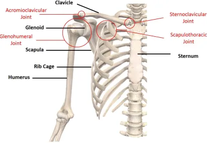
The four following articulations are the main constituents of the shoulder: the
glenohumeral joint, sternoclavicular joint, acromioclavicular joint, and scapulothoracic
joint (Figure 1.2). The bones that are involved in creating these articulations are the
humerus, scapula, clavicle, sternum, and ribs. Moreover, the clavicle (collarbone) is also
involved in forming the shoulder complex. These articulations act in concert to restrain any
unintended movement and allow necessary motion of the shoulder [16]. Located between
the humeral head and the glenoid concavity of the scapula, the glenohumeral joint is the
major articulation of the shoulder contributing the most to shoulder ROM and the primary
articulation of interest in this study.
Figure 1.2 Bones and articulations of the shoulder (Image courtesy of Complete
1.1.1.1
Joints
The glenohumeral joint is the major articulation of all the joints in the shoulder. Being
called the ‘shoulder joint’ in many common usages, it is situated in between the humeral
head and the glenoid concavity of the scapula (Figure 1.2). This particular joint has the
largest ROM compared to all other joints of the body [18]–[22]. Therefore, in order to
conduct any research concerning the shoulder joint or its replacement for that matter, it is
imperative to clearly identify and study glenohumeral contact forces. Numerous studies in
the literature have done so by investigating the in vitro glenohumeral contact forces [23]–
[25] or alternatively using either two or three-dimensional musculoskeletal models [26],
[27].
Notwithstanding, some inconsistencies arise when one tries to calculate joint reaction
forces due to the variety of muscles and consequent indeterminacy. To address this,
Bergmann et al. [28] proposed and implemented an in vivo method of study that made
obtaining more plausible data possible through direct measurements from a telemeterized
implant that recorded the glenohumeral contact forces for different activities including
shoulder abduction and flexion.
1.1.1.2
Bones
Comprising the glenohumeral joint, the humerus is the most proximal bone of the upper
extremity. Its head is situated superior, medial and posterior with respect to the humeral
shaft and articulates with the glenoid and is geometrically close to one-third of a sphere
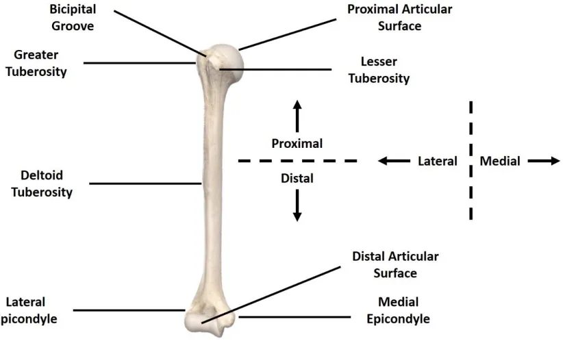
(Figure 1.2) [16]. Additionally, the humerus possesses several distinct landmarks: the
greater tuberosity (GT), lesser tuberosity (LT), the bicipital groove (between greater and
lesser tuberosities), the deltoid tuberosity, and the medial and lateral epicondyles (Figure
1.3). Being in the middle segment of the humeral shaft and on its lateral side, the deltoid
tuberosity is the distal insertion location of the deltoid muscle. In addition, the greater
tuberosity acts as the nexus of deltoid muscle insertion points on the humerus and its origin
located on the acromion of the scapula, enabling the deltoid activity even when the arm is
Figure 1.3 Bony Landmarks of the humerus (Image courtesy of Complete Anatomy
software, Dublin, Ireland)
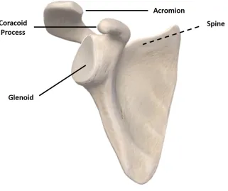
Another yet essential part of the shoulder joint, the scapula, is the triangular bone located
in the shoulder connecting the upper limb to the thorax and is also partly responsible for
the motion of the upper limb by being the origin for multiple muscles (Figure 1.4) [16].
Several bone projections such as the spine, acromion, and coracoid process emanate from
Figure 1.4 Bony landmarks of the scapula (The spine is located on the posterior side)
(Image courtesy of Complete Anatomy software, Dublin, Ireland)
These projections have variegated functions inside the shoulder. For instance, middle and
anterior deltoid and the trapezius muscles all originate from the acromion [16], while the
trapezius and the posterior deltoid muscles intersect at the scapular spine process.
Moreover, the scapula participates in the shoulder’s ROM through its gliding over the
ribcage, creating a 2:3 ratio of glenohumeral abduction/flexion angle to gross shoulder
abduction/flexion angle for most of its ROM [29], [30].
1.1.2
Soft Tissue Constructs
Many muscles surrounding the shoulder play a role in shoulder stabilization and
movement. It is possible to divide such muscles into three distinct categories as follows:
1. Axiohumeral muscles
2. The scapulohumeral muscles
The axiohumeral and axioscapular muscles emanate from the thoracic cage, but the
axiohumeral muscles insert on the humerus and axioscapular ones insert on the scapula.
Latissimus dorsi and pectoralis major muscles comprise the axiohumeral muscles while the
serratus anterior, the levator scapulaei, the trapezius, the pectoralis minor, and the
rhomboids all form the axioscapular muscles. The function of this muscle group is to
facilitate scapula motion. On the other hand, the scapulohumeral muscles, the muscle group
that emerges from the scapula toward the humerus, are composed of the deltoid, teres
major, teres minor, supraspinatus, subscapularis, infraspinatus, and coracobrachialis.
The deltoid muscle, which is responsible for humerus abduction by generating about half
of the elevation moment, is itself separated into three major parts, namely the anterior,
middle and posterior sections [31], with more contribution from the first two sections [16].
The posterior deltoid is involved in the external rotation and extension of the humerus,
while the anterior deltoid contribution is more involved with internal rotation and flexion
of the humerus [32].
The last relevant muscle group is the rotator cuff, attached to the greater tuberosity of the
humerus, and is made up of the joint capsule, the ligaments, the teres minor, subscapularis,
supraspinatus, and infraspinatus muscles and the tendons surrounding the glenohumeral
joint.
1.2
Structure and Material Properties of Shoulder Bones
1.2.1
Structure of Bone
Considered a composite material, bone consists of mineral substances and organic matter
with a 2:1 ratio, respectively. Working in concert, these two components bring about the
required strength and resilience for the bone. The mineral component makes a greater
contribution to the bone strength and resists compressive stress while the collagenous
organic component assists in resisting tensile stress and providing viscoelasticity to the
bone [33]–[35].
The bone is mainly responsible for bearing the body’s mass and the stresses applied to it.
a constant destructuring and restructuring cycle attributed to osteoclasts and osteoblasts,
which are responsible for bone tissue resorption and formation, in that order [38], [39].
Viewed at a macroscopic scale, the structural components of long bones, which constitute
the appendicular (i.e., arm, leg, etc.) skeleton, are divided into three sections: the diaphysis
(shaft), epiphysis (where the articulation is located), and metaphysis (between epiphysis
and diaphysis) [40]. Also, bones can be categorized as either cortical (compact) or as
trabecular (cancellous). Cortical bone is a relatively more homogenous and denser structure
when juxtaposed with cancellous bone. The epiphysis is, in essence, a cancellous bone
within a cortical shell, while diaphysis is a cortical shell with an inner medullary cavity, a
hollow canal containing the bone marrow. A porous, heterogenous and varying structure
in its entire volume, cancellous bone can contribute to local anatomic functions [34], [35],
[40]. Due to osteoporosis, which is a common bone illness, especially for aged populations,
the porosity of cortical and trabecular bone increases and, subsequently, the load-bearing
capability of the bone is reduced [41].
In the microscopic realm, the extended bone columns parallel to diaphysis called Osteons
constitute the cortical bone. On the contrary, the cancellous bone is made of trabeculae, a
set of extremely organized, dense, and aligned isolated struts of tissue. The orientation of
the trabeculae is so that they are positioned in line with the stresses applied to them [34].
1.2.2
Material Properties of Bone
Obtaining Young’s modulus, or associated stiffness is an integral part of the quantitative
analysis of bone elastic properties. Estimating the stiffness of bone is a complicated task
due to its heterogeneity, especially for trabecular bone. To address this, sophisticated
medical image processing methods are utilized to locally obtain the material properties of
bone in small regions termed voxels. In particular, computed tomography (CT) images can
provide x-ray attenuation data measured in Hounsfield units (HU). Then, based on a
quantitative relationship derived from bone calibration data, the apparent density (defined
The Young’s modulus can be estimated using the measured bone density. Numerous
studies have proposed equations relating Young’s modulus to bone density [43]–[47].
These equations mostly take into consideration both cortical and trabecular bones.
However, Morgan et al. [48] proposed a formula that yields Young’s modulus of trabecular
bone at various sites in the body utilizing an in vitro technique. Similarly, Austman et al.
[43] derived a relationship that correlates apparent bone density to Young’s modulus for
the cortical bone of the ulna. As was suggested by Zannoni et al. [42], by ascribing varying
Young’s modulus obtained from the CT scan HU data to each element of a mesh, the
heterogeneous properties of the bone can be approximated.
1.3
Shoulder Arthroplasty
The first-ever recorded instance of a shoulder replacement occurred in the early 1890s and
was successfully used towards treating fractures in proximal humerus while recovering
normal ROM of the shoulder and alleviating the associated pain [49]. In the 1970s, Neer
[50] expanded the domain of the usage of this method to treat a condition that severely
limits the optimal functioning of the shoulder, known as glenohumeral arthritis, which can
have many causes such as congenital, traumatic, vascular or septic factors, among others
[16], [50]. For addressing severe arthritis of the glenohumeral joint or fractures involving
the proximal humerus, shoulder arthroplasty is still the method of choice. Treatment
options include partial surface reconstruction, hemiarthroplasty, total shoulder arthroplasty
Figure 1.5 The main forms of shoulder reconstruction [51]
During TSA and RTSA, complete (two-sided) replacement of the glenohumeral joint with
a prosthesis is required [52].
Typically, a prosthesis designed for shoulder replacement can be divided into three
sections, namely, a humeral head, glenoid structure, and the implant stem. In the
hemiarthroplasty method, one-sided replacement of the humeral side of the joint with a
humeral head and an implant stem occurs, while in partial resurfacing, one of the joint
surfaces is replaced and native bone is mainly left intact [52].
Numerous breakthroughs have been made in implant design, materials used and methods
related to stabilizing and sterilization of prostheses as well as surgical procedures followed
More recently, modified implant designs have been proposed that are characterized by
either a reduced humeral stem length or having removed them completely. Usage of these
shorter versions of implant stems is becoming more commonplace because of the reduction
in broaching and reaming of the humeral canal they provide. This, in turn, results in higher
preservation of the original native bone while reducing the stress exerted on the cortical
bone and also rendering perioperative periprosthetic fracture less likely. As suggested by
various studies in the literature, reducing the length of the humeral stems is responsible for
the decrease in stress shielding by maintaining a larger portion of the original native bone
[54]–[57].
In order to fix the implant into the host bone and link the bone and prosthetic structures
together permanently, two main methods, namely, cemented and press-fit are currently
being employed. Based on the selection of fixation type, various surface textures such as
plasma spray, trabecular metal, grit blast or smooth polished may be used on the implant
for improving the biological reaction of the shoulder to the prosthesis [58]. More recently,
uncemented types are being preferred due to their longer stability caused by the
conservation of a greater portion of the native bone in this technique [59], [60].
Although shoulder implant design has made enormous progress, there are still some
challenges that need to be addressed. For instance, implant loosening, proximal bone loss,
fractures happening during or after the surgery, and stress shielding are obstacles that still
exist and are yet to be overcome [56], [61].
A study by Denard et al. [62] posits that while short stem implants generate less osteolysis
compared to regular stems, a significant portion of them, around 20 percent, still cause
cortical thinning of the lateral proximal metaphysis and half of them caused cortical
thinning of the medial metaphysis. The same study observes an additional 23% partial
calcar bone resorption in short stem models. Furthermore, once implanted, 86% of the short
stem models were anatomically aligned compared to 98% of regular stems. This increased
misalignment, in turn, can compromise shoulder functionality by causing stiffness in the
reported by Schnetzke et al. [64], and a rate of 83% of various forms of bone loss was
recorded using a sample study group of 52 short stem models.
Both Casagrande et al. [65], and Morwood et al. [66] indicate a list of problems associated
with using short stem models including an 8% revision rate due to humeral loosening in
patients, at least one humeral radiolucency in 71% of the implants, partial or complete
osteolysis on the medial calcar in 18% of the patients and radiolucencies in 21% of short
stem models.
Razfar et al. [67] also observed that although making use of short stem implants reduced
the average stress in cortical bone, trabecular bone stresses were elevated relative to the
standard stems.
Over 66,000 shoulder replacements are performed annually in the United States [6] and
over 4,000 annual shoulder replacements are performed in Canada [68]. Therefore, it is of
utmost importance to maintain the long term stability of the implant so as to retrieve normal
shoulder joint function and also preclude the occurrence of humeral revision because of the
established correlation between humeral revision and periprosthetic fractures, metaphyseal
bone loss and other complications [56].
1.4
Wolff’s Law and Stress Shielding
When an applied load on a specific portion of bone passes or drops below a certain
threshold, bone’s reaction includes resorption and remodeling itself. This effect, known as
Wolff’s law, plays an important role in reconstructed joints as the implant stem or its keel
partially bear some of the load applied to the bone [36]. Consequently, the original bone
stimulus is reduced and what is known as stress shielding occurs. This phenomenon, in
turn, can lead to bone resorption or implant loosening [69]–[71]. Nagels et al. [8] recorded
the occurrence of stress shielding in the vicinity of humeral implants in 9% of their sample
cases, which comprised of 70 implants. However, when restricted attention to cortical
bone, they estimated that the actual development of stress shielding around the shoulder
implants to be higher. Several other studies have also reported resorption of the bone near
Huiskes et al. [37] proposed a strain energy density-based method for bone adaptation and
characterized internal bone morphology by the apparent bone density. They stated that
when the strain energy density (SED) goes above a specific threshold, the bone density will
increase while the bone density will decrease when SED goes below the threshold. They
proposed that the rate of bone adaptation is proportional to the amount of increase/decrease
of SED beyond the threshold. This energy is, in essence, the internal work (strain energy)
balancing the external work done by the externally applied force on an object. SED can be
computed using Equation1.1
𝑆𝐸𝐷 = 𝜎2
2𝐸 (Equation 1.1)
If the object of interest is linear isotropic that bears small strains, SED can be obtained via
Equation 1.2
𝑆𝐸𝐷 = 1
2 (𝜎𝑥𝜀𝑥 + 𝜎𝑦𝜀𝑦 + 𝜎𝑧𝜀𝑧 + 2𝜎𝑥𝑦𝜀𝑥𝑦 + 2𝜎𝑦𝑧𝜀𝑦𝑧 + 2𝜎𝑥𝑧𝜀𝑥𝑧) (Equation 1.2)
Where 𝜎 and 𝜀 show the components of stress and strain tensors, respectively.
Bone adaptations have shown to be well correlated with changes in SED [73], [74]. By
comparing two different techniques of SED-based bone remodeling and compliance-based
structural topology optimization from a mathematical formulation perspective, Jang et al.
[75] showed that the SED-based bone remodeling technique could be mathematically
formulated as a compliance-based structural topology optimization problem. In structural
topology optimization material is mapped in a design domain systematically and iteratively
such that an optimal structure can be achieved, minimizing a predefined objective function.
It is possible to obtain an accurate prediction of the density distribution of the bone in
response to external loads by using iterative computer models based on SED
measurements, and thus estimate the response of the bone to arthroplasty [37], [73], [76],
[77]. Neuert et al. [73] modeled human ulna from micro computed-tomography (𝜇CT) data
using the SED-based bone remodeling technique. They considered an initial uniform
density distribution for the bone and exerted loads based on in vivo data. Different threshold
density distribution was contrasted with 𝜇CT data. The optimal model parameters were
then utilized to model six additional human ulnae. They found that the SED threshold as a
variance of 55% from the bone’s natural SED, results in the smallest error between
estimated and physiological density values. Moreover, Reeves et al. [78] used an
SED-based bone remodeling algorithm to predict humeral bone initial response to shoulder
arthroplasty.
1.5
Statistical Shape and Density Modeling
The enormous variability in anatomical and biomechanical characteristics of biological
structures such as material properties, joint kinematics and dynamics, and geometry can be
challenging from a medical device design or surgical planning point of view [79].
By using statistical shape models (SSM), and statistical shape and density models (SSDM),
the morphological and mechanical variability can be quantitatively analyzed respectively
via attaining the average bone shape and average bone density and their main variation
modes within a population. Certainly, the accuracy of the predictions of the variation
among subjects resulting from any model is contingent upon the selected sample size and
the explanatory power of it in terms of representing the population. One advantage of the
SSM method is the fact that it can determine the variability in anatomical features of a
subpopulation that share the same background [80]. Examples of such subpopulations are
individuals with osteoporotic or osteoarthritic conditions or those who share common sex
or ethnicity. This feature can allow medical specialists and clinicians to more accurately
diagnose diseases and plan the treatment or surgical procedures required and also assist
engineers in the design process of medical equipment.
In practice, while it is ideal to have models specifically designed for each individual to
address personalized medical needs, time and financial constraints always exist. SSM is
capable of decreasing the instances where such costly models are required or at a minimum,
render their design less expensive by reducing computational time. As such, SSM has been
in use as a predictive tool. For instance, it can be employed to predict the shape of the
shoulder joint from adjacent segments [81]. Additionally, as an example, SSM has
including contact mechanics and kinematics, by analyzing joint shape on patellofemoral
and tibiofemoral sides [82], [83].
Numerous studies suggest an alternative usage for SSM, which involves reconstruction of
the 3D geometry of bones and cartilages by an automated segmentation of CT or magnetic
resonance images eliminating inter- and intra-observer errors [84]–[86].
Until now, much attention has been given to SSM in the literature in different bones
throughout the body. Instances of such studies include the humerus [87] or pelvis [88].
They have also been applied to human joints, including the shoulder [81], [89], knee [82],
[83], [85], and the spine [90]. However, SSDM has been often neglected in comparison,
and only a few studies have used this tool [91]–[93]. Even among these, the common theme
is their confined focus on the femur. In order to procure an SSDM of a bone, the
mainstream technique in practice is to derive the apparent bone density from CT image
values [94] and use the obtained results to subsequently estimate the Young’s modulus
through a set of experimental formulae as found in studies such as [48], [95]. Design and
size determinations of medical devices can be addressed by SSM for any population or
subpopulation having similar morphological traits [96], while SSDM can help test these
designs due to their ability to create population-based finite element (FE) models of the
bone structures along with their associated material distribution. In orthopedics and other
medical fields, such finite element models are becoming more commonplace before
introducing medical products into the market. FE analyses can be used to predict the
distribution of stress or fatigue life in the implanted bone [97], which in turn reduces the
associated costs and time needed for in vivo or in vitro experiments. Furthermore, the effect
of implants on the biomechanics of the joint can be estimated using the SSDM, a task that
is quite challenging in experiments, especially in measuring muscles, ligaments or internal
contact forces [85], [98], [99]. Finally, the intricate and tedious process of the construction
of FE models can be greatly shortened by utilizing the SSDM of the bone, rendering this
method an increasingly popular option in the manufacturing of medical devices [90].
Both SSM and SSDM can be considered as versatile and powerful platforms that allow a
variability of the bones by taking into account an entire spectrum of probable outcomes
through expanding the original training set. The size of the training set at hand is directly
correlated with the amount of anatomical variation SSM and SSDM can explain within a
population. For this purpose, a principal component analysis initiates SSM and SSDM to
avoid the difficulties accompanying identifying main independent variation modes in large
data sets. This statistical procedure diminishes the original data set at hand in terms of its
dimension while maintaining the same level of variation contained in it [100].
1.6
Finite Element Simulation of Shoulder Arthroplasty
Joint forces, movements, and anatomy are increasingly being simulated by the FE analysis
method, a subcategory of in silico techniques. The FE approach is, in essence, the
discretization of a solid continuum into a finite number of smaller elements that are joined
together at nodes. This unit consisting of nodes and elements, constitutes what is known as
a mesh. The method then proceeds to predict the characteristics of the entire system using
localized data. In particular, the applied load, material properties of the system investigated
and boundary conditions determine the displacements at each individual node. To further
facilitate the incorporation of the variability present in these factors, the values of these
parameters can be adjusted for each specific mesh.
On the contrary, more expensive and time-consuming in vitro experiments are only useful
for localized and isolated analyses, and their predictions cannot be extrapolated accurately
to other parts of the bone.
The selection of mesh size is an essential phase of any FE analysis as the accuracy of the
FE technique hinges upon mesh resolution, which in itself is a function of the mesh size.
However, a trade-off exists between the accuracy of the results, which increases with the
number of elements and the computational load associated with the higher number of
equations needed. Therefore, an optimal number of elements would be small enough to
provide adequate accuracy while not being severely time-consuming for the computation
devices. The process that enables the determination of this optimal mesh size is known as
First- and second-order tetrahedral/hexahedral elements can be used to generate FE volume
meshes. In the case of curved boundary zones, second-order (quadratic) elements perform
more favorably compared to first-order (linear) ones. Some studies present in the literature
indicate that the second-order tetrahedral mesh configuration provides more accurate
estimates [101], [102].
Following the discretization step and generation of the meshes, modeling parameters such
as load characteristics, element material properties, and boundary conditions are inserted
into the model. After that, the displacements attributed to each individual node can be
provided by an FE analysis software suite, such as ABAQUS 2018 (Dassault Systèmes,
Johnston, RI, USA), which was utilized in this study. Finally, all recorded stresses, strains
and other relevant data can be rendered for interpretations. Advanced FE software
empowers the researchers in the field of biomechanics, tasked with implant design, to test
numerous design configurations by adjusting design factors such as bone geometry,
implant design, material properties and loading conditions [103], [104].
1.7
Project Scope and Objectives
This study aims to contribute to enhancing the performance of shoulder replacement
implants by firstly providing a better understanding of how shoulder’s shapes and densities
vary among members of a population by utilizing statistical shape and density modeling.
Secondly, the gained insight was leveraged toward investigating the ability of hollow
stemmed-implants in limiting the stress shielding of proximal humerus by performing
finite element analysis.
Therefore, the objectives of this study are as follows:
1. To develop a statistical shape model and a statistical density model for the shoulder, and
to correlate main modes of its shape and density variation with available demographic data;
specifically, sex and age.
2. To determine if hollow titanium stems can mitigate stress shielding in comparison with
solid stems at the proximal humerus for a variety of bone qualities using finite element
1.8
Thesis Overview
Chapter 2 describes steps taken toward developing our statistical shape and density models
and correlations found between the main modes of shape and density variations and
demographic data such as age and sex. Also, the symmetry of contralateral shoulders in
terms of shape and density are discussed. Chapter 3 examines the implications of using
hollow-stemmed implants on changes in the stress distribution of bone and percentage of
bone volume with resorption/formation potential following bone reconstruction. Chapter 4
summarizes the findings of chapters 2 and 3, mentions the strength and limitations of this
work and outlines future directions. Supplementary information regarding chapter 2 can be
Chapter 2
2
Investigating the Effects of Demographics on the Shape
and Density of the Shoulder
This chapter describes steps taken toward developing our statistical shape and density
models and correlations found between the main modes of shape and density variations
and demographic data such as age and sex. Also, the symmetry of contralateral shoulders
in terms of shape and density are discussed.
2.1
Introduction
Total shoulder arthroplasty (TSA) is widely regarded as a clinically successful surgery used
to relieve pain or restore movement to an arthritic shoulder joint [1]–[3]. This has led to a
significant increase in its utilization over the past several decades [5], [105]–[107]. The
number of TSA and hemiarthroplasty procedures performed in the United States increased
from approximately 19,000 in 2000 [5] to more than 66,000 in 2011 [6]. The increasing
number of arthroplasty procedures, along with their increased charges, can impose a
financial burden on the health care system [7]. The most technically complicated class of
shoulder arthroplasty is the revision of a failed TSA, as various factors can lead to failure
[108]. As the number of TSA procedures increases, the need for revision surgeries also
rises [109]. In the United States, the revision burden for upper extremity arthroplasty
increased from 4.5% in 1993 to approximately 7% in 2007 [7]. Also, the revision rates for
TSA grew by 29% between 2006 and 2010 in France, while this rate was 10% for knee and
1% for hip implants in an identical period [110]. Poor bone quality around the implants, or
sub-optimal load transfer between implant components and surrounding bone, may affect
long-term fixation and ultimately lead to implant loosening and the need for revision
surgeries [108], [111].
Therefore, a better understanding of the normal and pathological bone shape and density
distribution in the proximal humerus and glenoid may help design implants with improved
bone-implant mechanics. Furthermore, tailoring implant shape/stiffness to match specific
patient sub-populations may result in a more suitable selection of implant shapes than a
of variation in the shape and density distribution of the shoulder in a population and the
demographics of that population would be beneficial.
SSM [112], and SDM [113] are tools capable of describing the shape and complex density
distribution of bones in terms of a relatively small set of uncorrelated variables called
principal components (PCs). PCs can describe the main modes along which the shape and
the spatial distribution of bone density can vary among the members of a population with
respect to the average shape and the average density distribution of that set. Describing the
shape and density distribution of a given bone by a small set of principal component
weighting factors, rather than using physical descriptors, can be more accurate and
efficient. Previously, SSMs have successfully been applied to describe the main modes of
variation in the shape of different organs such as the liver [114], [115], heart [116], [117],
and brain [118], [119]. Examples of bones and joints include the femur [120], hip [121],
[122] and knee joint [123]. Furthermore, SDMs have been applied to the femur [91], [93],
[113] and the mandibular condyle [124]. At the shoulder, there has been recent progress in
applying SSMs to characterize the variability of shapes at the shoulder joint [89], [125];
however, despite its importance for understanding the mechanics of bone-implant load
transfer, neither of these works considered the variability in the density distribution of the
shoulder.
Therefore, the objective of this study is to develop an SSM and an SDM for the shoulder,
and to correlate shape and density PC scores with available demographic data; specifically,
sex and age. We hypothesize that the main mode of shape variation in our SSM will be a
scaling factor related to the size of the bones. To that end, we theorize that males, on
average, have larger humeri and scapulae than females; however, well-matched individuals
by weight, height, BMI and age of a different sex will have similar size bones. Moreover,
the first PC of the SDMs will likely scale the density over the entire bone, and we anticipate
that this PC will be inversely correlated with age (due to natural bone density loss with
age) and will, on average, be greater for males than females. Finally, because we are
creating separate SSMs and SDMs for each of the humerus and scapula based on one
population, we also hypothesize that there will be correlations between several PCs of
2.2
Methods
2.2.1
Development of Statistical Shape and Density Models
Specimens
Separate SSMs and SDMs were created for the humerus and scapula using available
computed tomography (CT) scans of 75 human cadaveric shoulder joints. This set includes
57 male (20 pairs) and 18 female shoulders (1 pair) from 54 donors, with ages ranging
between 21 and 94 years (mean 73 ± 13). Heights ranged from 147 to 191 centimeters
(mean 173 ± 10), and weights ranged from 30 to 116 kilograms (mean 65 ± 18). Thus, the
shoulders in the set represented large anatomical and size variability with two donors were
noted to have osteoarthritis and one to have osteopenia.
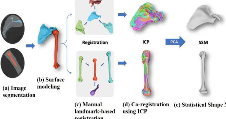
Figure 2.1 Steps taken toward developing SSMs from CT images
Three-Dimensional Model Reconstruction
Surface geometries of each scapula and humerus were segmented from CT scan data using
the 3D medical image processing software 3DSlicer [126] (Figure 2.1(a)). A
threshold-based segmentation protocol, threshold-based on previously described techniques, was employed for
each CT scan to label, reconstruct, smooth, and create triangle-tessellated models of each
and humerus bones, and triangular meshes were extracted for all the segmented 3D models.
Right-side scapulae and humeri data were reflected to be left-sided, to simplify the
development of the SSMs.
Co-registration and surface mapping
Further data processing was performed in MeshLab [128]. A baseline shape was chosen at
random for each of the scapula and humerus, after which they were re-meshed to obtain a
smooth and uniform topology with a mean edge-length of 0.6 mm. This resulted in meshes
with about 110,000 vertices and 230,000 faces for scapula and about 90,000 vertices and
170,000 faces for the humerus. The 3D meshes of the remaining scapulae and humeri were
imported separately into MeshLab and aligned to the baseline shapes. Registration was
performed in two steps, first manually using defined homologous points (Figure 2.1(c))
and then refined using an iterative closest point algorithm (Figure 2.1(d)). The two baseline
meshes were then mapped/morphed to each of the segmented and aligned meshes in the
scapulae, and humeri model sets using R3DS Wrap 3.2 (R3DS, Voronezh, Russia). This
process resulted in a mesh for each specimen with similar topology and identical vertex
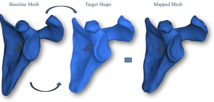
numbering but customized to the individual shape of each specimen (Figure 2.2). Having
the same topology simplified point-to-point comparison between the models.
Figure 2.2 Baseline mesh mapping (It was mapped to each of the aligned meshes to
Creating homologous volumetric meshes
Just as the humerus and scapula SSMs required a baseline surface mesh that could be
mapped or morphed to the shape of each individual specimen, the SDMs required a
baseline volumetric mesh, which could be fit into the individual surface mesh of each
specimen. This was achieved by first creating baseline humerus and scapula tetrahedral
element meshes in TetGen [129] from the same baseline specimen as in the SSMs. These
meshes used elements with mean edge-lengths of 0.7 mm, resulting in about 810,000 nodes
/4,800,000 elements for the humerus and about 460,000 nodes / 2,500,000 elements for the
scapula base meshes. These meshes were morphed to individual specimens by leveraging
the fact that identical surface mesh topologies already existed; thus, displacements, applied
directly to the surface nodes of the baseline model, could be used to match the surface to
any candidate model, and these displacements were distributed throughout the inner
volumetric mesh accordingly via the element shape functions and mesh connectivity. This
process resulted in a set of 75 corresponding shoulder mesh models.
Assigning nodal density properties
Each humerus and scapula mesh was then transformed back into its original CT coordinates
and imported into the open-source mesh pre-processing software MITK-GEM [130], along
with the corresponding CT data set. Using this software, the CT image intensity (in HU) at
each node location in the volume mesh could be computed from the CT data. As a result,
a set of 75 humerus and scapula 3D meshes, with homologous mesh topologies, each had
specimen-specific CT image intensity data assigned at each node. Due to the homologous
mesh topologies, the CT image intensity of any given node within a model could be
compared directly with the CT image intensity of the same node (at the same relative
position) within any other model.
Principal Component Analysis
The vertex coordinate data for all specimen models were imported into MATLAB R2017b
(Mathworks Inc., Natick, MA, USA) as point clouds, where the coordinates for all n
(𝑥1, 𝑦1, 𝑧1, . . . , 𝑥𝑛, 𝑦𝑛, 𝑧𝑛). Each vector represented the point coordinates for a single
specimen, and all were assembled into a single matrix (but a separate matrix for the
humerus and scapula coordinate data). Principal component analyses (PCAs) were
performed separately for the assembled humerus and scapula coordinate matrices to
identify principal components (PCs) of the shape for the humerus and scapula. These PCs
described the main modes of shape variation within each set most efficiently and were used
to find the average shape of the bones (Figure 2.1(e)).
In a similar manner, PCA was also performed on the spatial distribution of bones’ densities
to identify main modes of density variation within each set of the humeri and scapulae
separately.
Defining positive direction of PCs
In order to have a consistent definition for the positive direction of each individual PC of
the SSMs, all the specimens were sorted based on their volume in ascending order and
evenly split into two groups (high volume and low volume). The positive direction of each
PC was defined such that the corresponding PC score of the high-volume group would be
greater (more positive) than the corresponding PC score of the low-volume group.
Similarly, to establish a consistent direction of each individual PC of the SDMs, specimens
were sorted based on their average density over their entire volume in an ascending order,
divided into two equal groups (high density and low density), and the positive directions
of PCs were defined such that the high-density group had a higher average PC score (more
positive) than the low-density group.
Evaluating compactness and robustness of statistical models
A primary objective of statistical models (and PCA in general) is to use a compact set of
parameters (fewer parameters) to describe variability in a set. To evaluate the compactness
of models, the percentage of variability between meshes in the set explained by each PC
was calculated for SSMs and SDMs for each of the humerus and scapula. Furthermore, for
each specimen, the error in reconstructing the shape and density distribution of the humerus
The robustness of the SSMs (Appendix B) and SDMs (Appendix C) against the particular
specimens used in the study was also assessed.
2.2.2
Data Analysis
The shape and density of the humerus and scapula, as described using principal
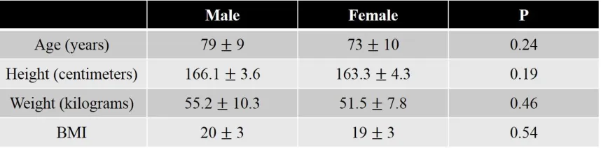
components, were compared for males versus females. To reduce the bias of the larger
average male subject sizes, a more comparable sub-group of males and females in the
height range of 157 to 170 centimeters was chosen, which included 7 male and 11 female
donors. The age, height, weight and BMI of these donor sets were not significantly different
(Table 2.1).
Table 2.1 The demographic data for male and female sub-groups
To test the hypothesis that the shapes of the humeri and scapulae from well-matched male
and female donor subsets were the same, student’s t-tests were used to compare the shape
and density PC scores of the humeri/scapulae of the well-matched male versus female
subsets (excluding contralateral bones) and statistically significant differences were
determined (p ≤ 0.05). To test the hypothesis that bone density will decrease with age,
Pearson correlation coefficients were calculated for age and PC scores of all the specimens
in the SDM (excluding contralateral bones).
Furthermore, since contralateral specimens were included in the study set, shape and
density PC scores of another sub-group containing 21 pairs of contralateral humeri and
scapulae were analyzed using paired t-tests in order to identify asymmetry in bone shapes
or densities. As information regarding the dominant hand of the donors was not available,
of the SSM and PCs of the SDM were calculated for each of the humerus and scapula
separately. Each statistical analysis using SSM/SDM data only included the first few
principal components, as determined by the results of compactness analysis.
2.3
Results
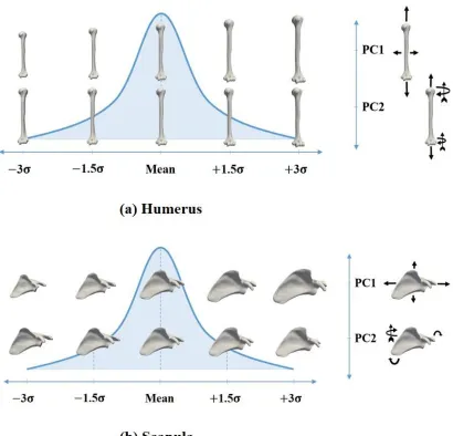
Main Modes of Shape and Density Variations
For the SSMs, the first mode of shape variation, as predicted, was a scaling factor in the
model set and the second mode correlated to the orientation of the bones as shown by the
arrows (Figure 2.3).
For the SDMs, the first mode of density variation scaled the density over the entire bone
Figure 2.3 The first two modes of shape variation of the shoulder; (a) for the
humerus, (b) for the scapula (Arrows with a vane at the end show the directions of
out-of-plane rotations)
SSM and SDM compactness
Using the SSMs, the highly correlated nodal coordinates of the shapes were reduced into a
relatively small set of 74 uncorrelated and independent shape variables (SSM PCs).
Similarly, using the SDMs, the highly correlated nodal density variables were reduced into
To assess the compactness of the SSMs and SDMs, the percentage of variability between
meshes in the training set accounted for by each PC was calculated for both the humerus
and scapula (Figure 2.4).
Each statistical analysis using SSM / SDM data only included the first few principal
components, which cumulatively accounted for 95% / 50% of the variability in the set as
almost all 74 PCs were required in order to describe more than 95% of the variability in
the SDMs (required 64 PCs for the scapula, and 61 PCs for the humerus). However, by
reconstructing specimens in the set, using a few numbers of PCs, we were able to capture
the pattern of density distribution for each specimen (Appendix A).
Ultimately, all statistical analyses of the scapula SSM and SDM data included the first 14
PCs of either model, which cumulatively explained 95.1% and 51.5% of the variability in
those models, respectively. All statistical analyses of the humerus SSM and SDM data
included the first 6 PCs of either model, which cumulatively explained 95.7% and 51.8%
Figure 2.4 Cumulative sum of the variability percentage explained by the respective
Sex Analysis
The mean shape of both scapula and humerus is shown in (Figure 2.5), which also shows
the average male and female scapula and humerus shapes resulting from the well-matched
subsets. Comparing the bone shapes (Figure 2.5 (d)), the male bones in the well-matched
set have, on average, a longer medial/inferior border and acromion of the scapula, and a
larger humeral head when compared to the average female shape.
Figure 2.5The shape of the humerus and scapula averaged over the entire
population and averaged over male/female sub-group (These sub-groups were
well-matched for age, height, weight, and BMI as explained in Table 2.1)
The PC scores of the SSM for male versus female humeri (Figure 2.6) and scapulae (Figure
2.7) in this set, were compared. For the humerus, statistically significant differences were
identified in PCs 3 and 5 of the SSM, with average PC scores differing by +1.4 ± 0.3 and
+1.0 ± 0.3 standard deviations, respectively, for males relative to the females (all p ≤ 0.01).
Statistically significant differences were identified in PCs 1, 2, and 9 for the scapula SSM,
with average PC scores differing by +1.3 ± 0.2, −1.1 ± 0.4, and −0.9 ± 0.4 standard
Figure 2.6The boxplot of the PC scores of male and female humeri in the
well-matched set for shape (Green: PC scores of male humeri, yellow: PC scores of female
humeri). The boxes represent the 1st to the 3rd quartiles, whiskers represent the range, lines in the box represent the median values, and squares represent the mean values of the
PC scores. The blue icons show the average humerus shape deviated along the
corresponding PC by +3σ, while the red icons show the same for deviations by -3σ. The
arrows show the effect of each PC on the shape of the humerus along the positive
direction of that PC (Arrows with a vane at the end show the directions of out-of-plane
Figure 2.7The boxplot of the PC scores of male and female scapulae in the
well-matched set for shape (Green: PC scores of male scapulae, yellow: PC scores of female
scapulae). The boxes represent the 1st to the 3rd quartiles, whiskers represent the range, lines in the box represent the median values, and squares represent the mean values of the
PC scores. Only the first 9 PCs, of the 14 used for statistical analyses, are shown for
brevity. The blue icons show the average scapula shape deviated along the corresponding
PC by +3σ, while the red icons show the same for deviations by -3σ. The arrows show
the effect of each PC on the shape of the scapula along the positive direction of that PC
(Arrows with a vane at the end show the directions of out-of-plane rotations).
The PC scores of the SDM for male versus female humerus (Figure 2.8) and scapula
(Figure 2.9) were compared as well. For the humerus, statistically significant differences
were identified in PC 2, 3, and 5 with average PC scores differing by −1.1 ± 0.5, +1.2 ±
0.4, and −1.2 ± 0.4 standard deviations, respectively for males relative to the females (all
p ≤ 0.04). For the scapula, statistically significant differences were identified in PC 2 of
the SDM, with average PC scores differing by −1.2 ± 0.5 standard deviations, for males
Figure 2.8The boxplot of the PC scores of male and female humeri in the
well-matched set for density (Green: PC scores of male humeri, yellow: PC scores of female
humeri). The boxes represent the 1st to the 3rd quartiles, whiskers represent the range,
lines in the box represent the median values, and squares represent the mean values of the
Figure 2.9 The Boxplot of the PC scores of male and female scapulae in the
well-matched set for density (Green: PC scores of male scapulae, yellow: PC scores of
female scapulae). The boxes represent the 1st to the 3rd quartiles, whiskers represent the
range, lines in the box represent the median values, and squares represent the mean
values of the PC scores. Only the first 9 PCs, of the 14 used for statistical analyses, are
shown for brevity.
The density distribution of the average male and female humerus and glenoid in the
well-matched set using all the PCs were compared (Figure 2.10). It can be seen that male
Figure 2.10Comparing the male with female bone density distribution (Left: male,
right: female). They were averaged over the well-matched set and mapped to the overall
average bone shape; (a) for the humerus, (b) for the glenoid
Age Analysis
For the humerus, the first and sixth PCs of the SDM demonstrated a weak [131] and
both p ≤ 0.03). For the ten youngest specimens, the averages of the first and sixth PC scores
were greater than that of the ten oldest by 1.0 and 0.5 standard deviation, respectively. For
the scapula, the first and ninth PCs showed such weak, but significant, correlations (ρ =
−0.31, and ρ =−0.32, both p ≤ 0.02). For the ten youngest specimens, the averages of the
first and ninth PC scores were greater than that of the ten oldest by 1.0 and 0.9 standard
deviation, respectively. No other significant correlation was observed for other PCs with
age.
Pairs Analysis
Using paired t-tests, PC scores of the SSM & SDM for paired right versus left shoulders
for both the humerus and scapula were compared. For the humerus SSM, statistically
significant differences were observed in PC 2, 4, and 5 with average PC scores differing
by +0.4 ± 0.9, +0.5 ± 1.0, and −0.5 ± 0.9 standard deviations, respectively for right humeri
relative to the left ones (all p ≤ 0.04). For the scapula, statistically significant differences
were identified in PCs 4 and 8 of the SSM, with average PC scores differing by +0.4 ± 0.6,
and +0.3 ± 0.5 standard deviations, for right scapulae relative to lefts (all p ≤ 0.01). For the
humerus SDM, PC 1 was significantly different, with average PC score differing by −0.3
± 0.7 standard deviation, for right humeri relative to the lefts (p ≤ 0.03). For the scapula,
statistically significant differences were observed in PCs 2 and 13 of the SDM, with
average PC scores differing by −0.4 ± 0.8, and −0.3 ± 0.7 standard deviations, for right
scapulae relative to the lefts (all p ≤ 0.03).
Correlation between SSM/SDM
Finally, there were weak, but statistically significant, correlations between several PCs of
shape and density. For both bones, the first PC of the SSMs, which is generally an overall
size scaling factor, showed a weak but, significant correlation, with the second PC of the
SDM, which generally influences the thickness of the cortical shell (ρ = −0.25, p ≤ 0.03 for
the humerus, and ρ = −0.39, p ≤ 0.001 for the scapula). Also, the first PC of the SSM &
SDM for the humerus showed such a correlation. (ρ = 0.31, p ≤ 0.01). The first PC of the
![Figure 1.1 Three common planes used to define anatomy [17]](https://thumb-us.123doks.com/thumbv2/123dok_us/1908484.1250083/13.612.187.483.219.524/figure-common-planes-used-define-anatomy.webp)
![Figure 1.5 The main forms of shoulder reconstruction [51]](https://thumb-us.123doks.com/thumbv2/123dok_us/1908484.1250083/21.612.120.539.76.415/figure-main-forms-shoulder-reconstruction.webp)