Exploring the Estimability of Mark-Recapture Models with Individual, Time-Varying Covariates using the Scaled Logit Link Function

(1)

Western University Western University

Scholarship@Western

Electronic Thesis and Dissertation Repository

8-2-2019 10:30 AM

Exploring the Estimability of Mark-Recapture Models with

Individual, Time-Varying Covariates using the Scaled Logit Link

Function

Jiaqi Mu

The University of Western Ontario

Supervisor Bonner, Simon J.

The University of Western Ontario

Graduate Program in Statistics and Actuarial Sciences

A thesis submitted in partial fulfillment of the requirements for the degree in Master of Science © Jiaqi Mu 2019

Follow this and additional works at: https://ir.lib.uwo.ca/etd

Part of the Biostatistics Commons, and the Statistical Models Commons

Recommended Citation Recommended Citation

Mu, Jiaqi, "Exploring the Estimability of Mark-Recapture Models with Individual, Time-Varying Covariates using the Scaled Logit Link Function" (2019). Electronic Thesis and Dissertation Repository. 6385.

https://ir.lib.uwo.ca/etd/6385

This Dissertation/Thesis is brought to you for free and open access by Scholarship@Western. It has been accepted for inclusion in Electronic Thesis and Dissertation Repository by an authorized administrator of

(2)

Mark-recapture studies are often used to estimate the survival of individuals in a population

and identify factors that affect survival in order to understand how the population might be

impacted by changing conditions. Factors that vary between individuals and over time, such

as body mass, present a challenge because they can only be observed when an individual is

captured. Several models have been proposed to deal with this missing-covariate problem

and commonly impose a logit link function which implies that the survival probability varies

between 0 and 1. In this thesis I explore the estimability of four possible models when survival

is linked to the covariate through a scaled logit link function which imposes some upper limit,

c < 1. Through a combination of theoretical analysis and simulation I show that the binomial

model is not estimable under the scaled link while the other three models remain estimable.

Keywords: model estimability, scaled logit link function, missing data, maximum

likeli-hood, Bayesian inference

(3)

Summary

Wildlife conservation has become a global task in the past few decades. A large number of

studies and field experiments have been conducted to assist in wildlife management and

con-servation. Ecologists are often interested in monitoring the abundance or understanding factors

that affect survival of an animal population, and have proposed many statistical models to study

these properties.

The Cormack-Jolly-Seber (CJS) model with covariates is often used to estimate the survival

of individuals in a population and identify factors that affect survival in order to understand

how individuals might behave differently and how the population might be affected by

chang-ing conditions. Factors that vary between individuals and over time, like body mass, present

a challenge because they can only be observed when an individual is captured. Several

exten-sions of the CJS models have been proposed to deal with the missing-covariate problem and to

understand the effects that a factor may have on survival even when it cannot be observed at all

times for all individuals. Moreover, these models all impose the assumption that the survival

probability varies between 0 and 1.

In this thesis, I examine the behaviour of the different models when the survival probability

is modeled via a scaled logit link function that restricts the survival probability to be less

than some constant, c < 1, that must be estimated from the data. In particular, I explore

the estimability of four possible models: the binomial model, trinomial model, full-likelihood

model, and alternative trinomial model. Through a combination of theoretical analysis and

simulation I show that effects of an individual time-varying covariate on survival cannot be

estimated from the binomial model when survival is scaled to be less than somec< 1, but the

other three models remain estimable. For me, the work in the thesis is important because it

helps us to understand what types of models we can use, and what type of data biologists need

to collect, in order to examine the effects of different types of factors that may have a significant

impact on individual survival and, hence, the sustainability of wild animal populations.

(4)

In the process of writing this thesis, I received a great deal of support and assistance. I would

first like to thank my supervisor, Dr. Simon Bonner, for presenting the ideas behind the thesis

and helping me solve the problems I encountered. He always encouraged me and pushed me

forward. Then I would like to thank Dr. Wei Zhang, for his helpful advice and comments on

my thesis.

I really enjoyed my time at the Western University. I want to thank my friends and

class-mates who have brought me a lot of fun in my study life. In addition, I want to thank my

parents who gave me unconditional support and love.

(5)

List of Figures

1.1 The structure of the CJS model. . . 7

1.2 The structure of the CJS model with covariates. . . 10

2.1 The structure of the alternative model. . . 24

3.1 The log-likelihood value of the Binomial model under the scaled link function

with the scalarc. The black line is the profile log-likelihood value as a function

ofcfor the Binomial model. The blue line is the true value ofc(c= 0.8). . . . 31

3.2 The estimates of capture probability pof the Binomial model under the scaled

link function with the scalarc. The blue line is the estimate of pas a function

ofc for the Binomial model. The red line is the product of the estimate of p

andc. . . 32

3.3 The log-likelihood value of the Trinomial model under the scaled link function

with the scalarc. The black line is the profile log-likelihood value as a function

of c for the Trinomial model. The blue line is the true value of c (c = 0.8).

The red solid line is the mle ofc. The two dashed red lines indicates the 95%

confidence interval of ˆc. . . 33

3.4 Posterior density ofcfor three models based on Bayesian inference. The black

line is the true value ofc(c=0.8). . . 35

3.5 Posterior density of cof different prior distributions for three models: the

bi-nomial model (A), the alternative tribi-nomial model (B), and the full likelihood

model (C). The black line is the true value ofc(c=0.8). . . 36

(8)

Introduction

1.1 Overview

Wildlife conservation has become a worldwide task in the past decades. A lot of research and

fieldwork have been done to help with wildlife management and protection. In wildlife

re-search, one is often interested in the abundance or survival of an animal population. Since it

is unrealistic to count or observe all individuals in the population, one first conducts

experi-ments to study the population of interest. Statistical models are then developed to analyze the

data from the experiment. Over the past century, capture-recapture (CR) methods have been

widely used to estimate the abundance (i.e., the total number of animals in a population) or

other demographic parameters (e.g., survival probability). This CR method is also the basis of

other more complex models, which can obtain some auxiliary information (e.g., individual

co-variates) to estimate relevant parameters more accurately. Many statistical and computational

techniques can be applied to these models to deal with more complicated cases and improve

the accuracy of the parameter estimation, which is an active research area.

In this thesis, I focus on extensions of the Cormack-Jolly-Seber (CJS) model (Cormack,

1964; Jolly, 1965; Seber, 1965) where survival probability is linked to an individual,

continu-ous, and time-dependent covariate. For example, I am interested in how an individual’s body

mass influences the survival probability which usually uses a logit link function to explore the

relationship. However, covariates are missing if individuals are not captured on some

(9)

1.1. Overview 3

sions. In this case, the survival probabilities cannot be expressed in terms of covariates, thus

we fail to write down the likelihood function for the CJS model.

So far, two methods have been developed to deal with the missing-covariate problem. One

is deleting unknown terms in the likelihood function such as the trinomial model based on the

three-state process for mark-recapture-recovery data (Catchpole et al., 2008). The other is the

full-likelihood approach which models the covariates to construct a likelihood function that can

be optimized by Monte Carlo EM (MCEM) algorithm or incorporated into a Bayesian analysis

(Bonner and Schwarz, 2006). Note that the MCEM algorithm is a modification of the EM

algorithm where the expectation in the E-step is computed numerically through Monte Carlo

simulation.

All of these previous methods assume that the survival is linked to the covariate through a

simple link function, by default the logit link, which assumes that survival can vary between

0 and 1. However, the logit link function can be questionable because we cannot promise the

individual will survive due to, for example, a large body mass. Instead, the scaled logit link

function has been chosen to explore the relationship between survival and covariate.

In similar work, Knape and Korner-Nievergelt (2015) showed that estimates of abundance

using the single-visit model with covariates of S´olymos et al. (2012) rely on accurately

spec-ifying the link function for detection probability. Their findings indicate that the choice of

the link function has a great impact on the estimation of parameters, and particularly that the

scaled link function makes it impossible to estimate the parameters of the basic single-visit

N-mixture models. For our problem, if we employ the scaled logit link function, the models

we investigate may become non-estimable – meaning that the data does not provide significant

information about the true parameter values. Futher details on the definition of estimability are

provided in Section 2.5.

The purpose of this thesis is to investigate the effects of using a scaled logit link function

on the estimability of the models developed to address the missing data problem that arises

(10)

are captured. I conduct simulations to explore the estimability of the binomial model, trinomial

model, alternative trinomial model, and full likelihood model.

1.2 Closed-Population Models

Closed-population models, whose main goal is to estimate the population size of the study

area, assume that no individuals enter the population by births or immigration or leave the

population through deaths or emigration during the experiment. Lincoln-Petersen estimator

(Lincoln et al., 1930), Chapman estimator (Chapman, 1951), and other more complex

closed-population models (Pollock, 1974) were proposed over the last century, which are based on the

capture-recapture experiment.

Capture-recapture (CR) is a popular method for estimating the abundance or other

demo-graphic parameters of an animal population (Pollock et al., 1990). The CR method is useful

when counting all individuals in a population is impractical. Pearson (1896) first used the

method to estimate the size of the population of plaice (Pleuronectes platessa) from the

Ger-man sea. Since then CR experiments have been used to study populations of Ger-many different

species. The same methods are also used in medical studies, and in the study of (Chartier

et al., 2015) to estimate the prevalence of chronic kidney disease based on cases defined in

ad-ministrative and laboratory data. Furthermore, CR data are typically a set of capture histories,

each of which is a string of binary digits of length K with 1 standing for capture and 0 for

non-capture. For example, an individual with history 01001 indicates that the individual was

captured on occasions 2 and 5, while not captured on other occasions in a 5-occasion study.

The Lincoln-Petersen (LP) estimator (Lincoln et al., 1930; Petersen, 1896) and the

Chap-man estimator (ChapChap-man, 1951) can be constructed from the simplest CR study, which only

consists of two capture occasions. On the first occasion, a sample of animals of size n1 is captured from the study area. Researchers put a unique tag on each of these animals and then

(11)

1.2. Closed-PopulationModels 5

rest of the population, another sample of sizen2, which is independent of the first sample, is captured. If the number of previously marked individuals in the second sample ism, then the

LP estimator is

ˆ

N = n1n2

m , (1.1)

where N denotes the population size, and we assume that the population is closed, being

marked does not affect the marked animals and the marks will not be lost. The LP

estima-tor is very simple but there are many limitations to this estimaestima-tor. For example, some species

are not easy to be observed such thatm = 0 or some small value. Chapman (1951) indicated

that the LP estimator is asymptotically unbiased as the sample size approaches infinity, but

is biased at small sample sizes and suggested an alternative estimator of population size, the

Chapman estimator:

ˆ

N = (n1+1)(n2+1)

m+1 −1, (1.2)

This is less biased than the Lincoln-Petersen estimator for small samples (Chapman, 1951).

In practice, to make more accurate inferences of the population, the closed-population

mod-els employ the CR data containing more than two capture occasions. Eight modmod-els were

pre-sented by Pollock (1974) and were fully developed by Otis et al. (1978). For example, the

simplest model, commonly referred to as model M0, assumes all individuals have the same probability p of being captured on all occasions. Let M denotes the number of individuals

captured at least one time during in the study, let K denote the number of occasions and let

nt denote the number of individuals captured on occasiont. The MLE (maximum likelihood

estimation) of the population size N can be found through solving equation (1.3) (Darroch,

1958):

1− M

N

=

K Y

t=1

1− nt

N

. (1.3)

(12)

maximizing the lnL(1.4) (Otis et al., 1978):

lnL= ln N! (N−M)!

! +        K X

t=1

nt       lnp+

      KN − K X

t=1

nt       ln (1

− p). (1.4) and then the MLE of pis

ˆ

p=

PK t=1nt

KN . (1.5)

1.3 Open-Population Models

Individual survival probability is a vital rate and often measured in the open-population CR

models. The open-population models allow individuals to die, be born, immigrate, and

emi-grate during the experiment. The Jolly-Seber model (Jolly, 1965; Seber, 1965) serves as the

starting point for open-population CR models which allows estimation of survival and

cap-ture probabilities, population size, and the number of new individuals entering the population.

In contrast, the Cormack-Jolly-Seber model is limited to estimation of survival and capture

probabilities, serves as the basis for the thesis and is described in the following paragraphs.

The Cormack-Jolly-Seber (CJS) model, formulated by Cormack (1964), Jolly (1965), and

Seber (1965), models the open-population CR data and is widely used in ecological studies.

By July 2019, Seber (1965) has been cited almost 2000 times according to Google Scholar.

Furthermore, many extensions to the CJS model have been developed. For example, in the

multi-state model, the capture and survival probabilities can change independently between

animals in a set of finite states defined by some factors (Arnason, 1973). Here I am interested

in models which allow the probability of survival to depend on continuous covariates that vary

between individuals and over time.

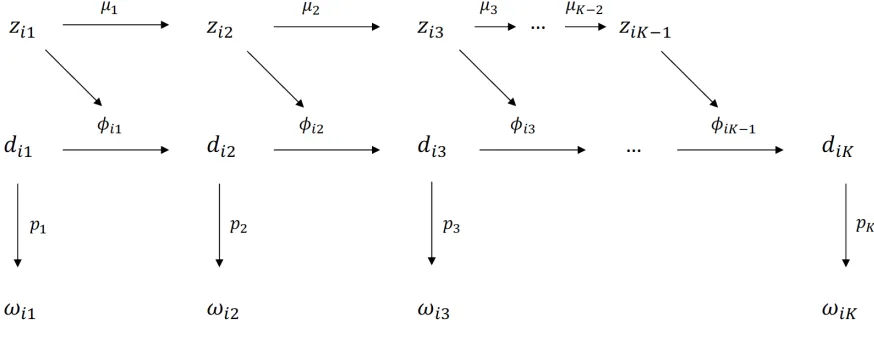
Let ωωωiii = (ωi1, ωi2, . . . , ωiK) denote the capture history of individual i, where ωit = 1 if

the individual was captured on occasion t(1 ≤ t ≤ K) and 0 otherwise, and letn denote the number of different individuals captured in the study. It is also useful to introduce a set of latent

(13)

1.3. Open-PopulationModels 7

is represented asdididi = (di1,di2, . . . ,diK) wheredit = 1 if individuali is alive and

PK

t=1ωit > 0,

anddit =0 otherwise.

The key assumptions of the CJS model are that all individuals alive on given capture

occa-sion are equally likely to be captured and equally likely to survive to the next occaocca-sion. More

specifically, the model assumes that (Williams et al., 2003):

1. Capture probability pt = P(ωi,t =1|di,t = 1) is the same for all individuals on occasiont.

2. Survival probabilityφt = P(di,t+1 =1|di,t = 1) is the same for all individuals on occasiont.

3. Marks are neither lost nor overlooked and are recorded correctly throughout the study.

4. Sampling periods are instananeous and recaptured individuals are released immediately.

5. Emigration from the study area is permanent.

6. Individuals are independent from each other.

7. Captures of the same individual on different occasions are independent.

Figure 1.1 illustrates the structure of the model for a single individual. Note that p1 cannot be estimated because the likelihood function for the CJS model (see equation (1.6)) conditions on

the first capture of each individual. Also, the final capture and survival probabilities, pK and

φK−1, are confounded and cannot be estimated separately.

Figure 1.1: The structure of the CJS model.

As an example, we consider an individual with capture history 01010. The likelihood

contribution for this individual is

(14)

and is formed as follows. First, we condition on the second occasion because that was when

the individual was first captured. We know that the individual survived from occasion two to

three and three to four, and the probabilities of these events areφ2andφ3. Also, the individual was alive but not captured on occasion three (probability 1− p3) and was alive and captured on occasion four (probability p4). On the last occasion, we don’t know whether the individual died or survived but simply was not captured. The combined probability of these two events is

(1−φ₄)+φ4(1−p5).

Since independence is assumed between individuals, the full likelihood for the whole set

of capture histories is the product of all these single conditional probabilities. Jolly (1965)

initially proposed method of moments type estimators for the capture and survival probabilities.

In fact, Jolly’s model also provides estimates of recruitment (birth and immigration). Seber

(1965) showed that the maximum likelihood estimators of capture and survival probabilities

have closed forms. Later, Bayesian inference was developed by Poole (2002). There are now

several stand-alone software packages available, for example, Program MARK (White and

Burnham, 1999), or packages for R, likemarked, (JeffLaake, 2018) that allow researchers to

fit the CJS model easily, obtain confidence intervals for the parameters, conduct hypothesis

testing (e.g.,p2 = p3 =· · ·= pK−1(Lebreton et al., 1992)), and perform model selection.

1.4 CJS Model with Covariates

Ecologists often wish to incorporate some measures as covariates to account for the situation

where assumptions of CJS model cannot be satisfied or more complicated situations arise. This

idea was first proposed by Pollock et al. (1984) to estimate capture probability for the

closed-population models. Pollock et al. (1984) linked the capture probability pt to a scalar variable

xt through the logit link function:

log pt 1− pt

!

(15)

1.4. CJS Model withCovariates 9

where β0 is the intercept and β1 is the slope. As we are interested in modeling the survival probability, model of Pollock et al. (1984) cannot be used because it assumes the population is

closed. Later Lebreton et al. (1992) described the CJS model with external variables through

the logit link function. Recall that the basic CJS model assumes that all individuals in the

population share the same survival probability on the same sampling occasion. However, this

assumption can be questionable in many situations because survival probability may depend

not only on extrinsic conditions but also intrinsic characteristics such as body mass, which may

vary between individuals and depend on sampling time. Williams et al. (2003) summarized all

possible covariates and classified them according to two descriptors: discrete vs continuous

and static vs dynamic. In my project, I am interested in modeling the effects of time-dependent

covariates (i.e., continuous and dynamic), which are stochastic for each individual.

For the CJS model with covariates, data consists of the normal CR data and the

correspond-ing covariates which are collected by measurcorrespond-ing the characteristic of each captured individual.

Suppose we consider a continuous, individual, and time-dependent covariate such as body

mass. Let zit denote the value of the covariate for individual i on occasiont, and let φit

de-note the survival probability from occasion t to t + 1 for individuali. Here we only model

the effect of the covariate on survival and assume that the capture probability pt is continuous

time-dependent but common to all individuals. Other variables are defined in the same manner

as for the CJS model.

A key difference between the basic CJS model and the CJS model with covariates is that

the survival probability for the latter is no longer assumed to be equal for all individuals on

each occasion. Since the survival probability lies between 0 and 1, it is natural to use a logit

link function to relate the survival probability to the covariate as we usually do for the logistic

regression model. Indeed, there are many other choices for the link function such as the probit

link functions, which are also widely used for generalized linear models. Under the logit link

function, we have

φ(zit|βββ)= exp(β0+β1zit) 1+exp(β0+β1zit)

(16)

for t = 1, . . . ,K −1. The model structure shown in Figure 1.2 is similar to that of the CJS model except the upper part, where the covariates are added.

Figure 1.2: The structure of the CJS model with covariates.

One considerable challenge of fitting the new model is that the covariate value,zit, can only

be observed if the individual is captured on occasion t, ωit = 1. Missing covariates prevent

the construction of the complete likelihood function, so the inference methods presented in the

last section cannot be applied. No matter which link function is used, we need the covariates

of all individuals on all occasions except for the last one. This is because the covariate on

the last occasion, ziK, only influences the survival probability φi,K+1, which is not involved in the likelihood of the model (Figure 1.2). Unfortunately, we have no way to collect covariate

information of an individual if it was not encountered on some occasions. For example, if

individualihas capture history 010010, then covariateszi3andzi4 are missing. We can ignore the fact thatzi6was not observed because it does not influence any survival probability. Due to the missing covariates (e.g., zi3 andzi4 in the above example), we cannot write down the full likelihood function. To deal with this problem, various methods were proposed. For instance,

Abraham and Russell (2004) developed a complete-case analysis which omitted all

individu-als involving missing covariates. Alternatively, Catchpole et al. (2004a) proposed a method

in which all missing covariates were replaced with the last available values. However, both

(17)

1.4. CJS Model withCovariates 11

models to handle missing covariates. These include three existing models: the binomial model

(Catchpole et al., 2004b), the trinomial model (Catchpole et al., 2008) and the full likelihood

model (Bonner, 2003). I also introduce an alternative model, which is a special case of the

(18)

Methodology

2.1 Binomial Model

The binomial model (Catchpole et al., 2004b) is based on the CJS model with covariates but

constructs the likelihood function by deleting all the unknown transitions which include

miss-ing covariates from the full likelihood function. As discussed in Section 1.4, missmiss-ing covariates

cause the problem that the corresponding survival probabilities cannot be calculated and thus

the full likelihood and parameter estimates cannot be obtained. Suppose individualihas

cap-ture history 101001. The likelihood contribution of this individual is

φi1(1− p2)φi2p3φi3(1− p4)φi4(1−p5)φi5p6. (2.1) Catchpole et al. (2008) considered a partial-case analysis by omitting all unknown terms from

the above likelihood contribution. Since this individual was not captured on occasions 2, 4,

and 5, covariateszi2, zi4, and zi5 were not recorded. Consequently, φi2, φi4, andφi5 cannot be computed and are removed from the full likelihood. Then the resulting reduced likelihood

contribution for this individual is

(19)

2.1. BinomialModel 13

The complete-case analysis (Abraham and Russell, 2004) simply omits all animals which have

any missing covariate. Compared to the complete-case analysis, the binomial model is less

biased because it only omits unknown transitions instead of all animals with missing covariates.

We introduce a two-state process to help derive the likelihood for the binomial model.

Recall that ωit=1 if the individual i was captured on occasion t and 0 otherwise. Define the transitionπi,t(a,b|ppp, βββ,zizizi) as:

πi,t(a,b|ppp, βββ,zizizi)=Pr(ωi,t+1= b|ωi,t = a, ωi,t−1, . . . , ωi,1,ppp, βββ,zizizi), a,b∈ {0,1}. (2.3) In addition, we defineχi,r,sto be the probability that individualiwas not captured from occasion

r+1 to sconditional on that it was alive at occasionr. Then we have the following recurrence

relation equation:

χi,r,s =(1−φi,r)+φi,r(1− pr+1)χi,r+1,s, ai ≤ r< s≤ K, (2.4)

where we letχi,r,r= 1. Now we have, forai ≤r≤ K−1,

πi,r(a,b|ppp, βββ,zizizi)=                             

φi,r(1− pr+1)+(1−φi,r) a=1,b=0

φi,rpr+1 a=1,b=1

χi,li,r,r+1/χi,li,r,r a=0,b=0

Qr−1

s=li,rφi,s(1− ps+1)φi,rpr+1/χi,li,r,r a=0,b=1

(2.5)

whereli,ris the last occasion on which an individual was captured before occasionr.

Using the transition probabilities defined above, the full likelihood function can be written

as:

L(ppp, βββ;zzz, ωωω))=

n Y

i=1

K−1

Y

r=ai

π(ωi,r, ωi,r+1|ppp, βββ,zizizi), (2.6) where ai = min{t : ωit = 1}and bi = max{t : ωit = 1} denote the first and last occasion on

(20)

The contribution of this history to the two-state likelihood is

thatφitcannot be obtained. For this reason, the transition probabilitiesπi,t(0,b|ppp, βββ,zizizi) (b= 0,1)

are unknown. Therefore,πi,2(0,1|ppp, βββ,zizizi), πi,4(0,0|ppp, βββ,zizizi), andπi,5(0,1|ppp, βββ,zizizi), which include φi,2,φi,4,andφi,5, cannot be computed through the logit link function. After that omitting these

three transitions from the likelihood, we have πi,1(1,0|ppp, βββ,zizizi) and πi,3(1,0|ppp, βββ,zizizi) left in the partial likelihood. Furthermore, the full likelihood presented by the equation (2.6) reduces to a

partial likelihood by removing all transitions starting from 0 for all captured individuals:

L(ppp, βββ;zzz, ωωω)=

n Y

i=1

Y

r∈{ai,...,K−1:ωi,r=1}

π(1, ωi,r+1|ppp, βββ,zizizi). (2.8) By maximizing this partial likelihood, we can find the maximum likelihood estimates (MLEs)

of the parameters.

2.2 Trinomial Model

The trinomial model (Catchpole et al., 2008) is used to analyze mark-recapture-recovery (MRR)

data with missing covariates for which the likelihood construction is based on a three-state

process. The trinomial model resembles the binomial model as they both delete unknown

tran-sitions in the likelihood, is easy to implement, and performs well according to the simulation

results of (Catchpole et al., 2008). The key difference is that the trinomial model analyzes the

MRR data.

MRR data comprise a set of capture histories that consist of a new state, the dead recovery

state 2 representing that an individual is found dead, in addition to the previously-defined states

(21)

2.2. TrinomialModel 15

values of lengthKwith 0 standing for non-capture, 1 for capture, and 2 for dead recovery. For

example, capture history 01020 denotes that the individual was first captured on occasion 2,

not encountered on occasion 3, and found dead on occasion 4.

The trinomial model involves all the assumptions of the CJS model with covariates and

two more assumptions for the state of dead recovery. One is that if an individual dies between

occasions t and t + 1, it is either found dead in this time interval or never found (i.e., the

individual cannot be found dead after occasion t+ 1). The other is that the dead recovery

probabilityλt = Pr(ωi,t = 2,di,t =0|di,t−1= 1) is the same for all individuals that die between occasionstandt+1. Under the trinomial model, we see that the individual with capture history

01020 was still alive on occasion 3, died between occasion 3 and 4, and was found dead with

probabilityλ3.

The full likelihood of the trinomial model conditional on the initial captures is (Catchpole

et al., 2008),

L(ppp, βββ, λλλ;zzz, ωωω)=

n Y

i=1

{(1−φi,bi)λbi}

di,biχ

i,bi

1−di,_bi

bi−1

Y

t=ai

{φi,tp wi,t

t+1(1− pt+1)

1−wi,t_}. _(2.9)

Similar to the basic CJS model with covariates, we cannot evaluate the likelihood (2.9) because

of missing covariates. To deal with this issue, Catchpole et al. (2008) introduced a

three-state process. Now the transitionsπi,t(a,b) andχi,r,s defined for the binomial model have new

expressions with a new state introduced. We add a “∗00to the top right corner of each transition to represent the new expressions. Let

χ∗

i,r,s=Pr(ωi,r+1=, . . . , ωi,s =0|di,r = 1)

=(1−φi,r)(1−λr)+φi,r(1− pr+1)χ∗i,r+1,s,

(22)

forai ≤ r< s≤ K withχ∗_i_,_r_,_r= 1.Then we have,

πi,r(a,b|ppp, βββ, λλλ,zizizi)∗=                                                       

φi,r(1− pr+1)+(1−φi,r)(1−λr) a=1,b=0

φi,rpr+1 a=1,b=1

(1−φi,r)λr a=1,b=2

χ∗

i,li,r,r+1/χ ∗

i,li,r,r a=0,b=0

Qr−1

s=li,rφi,s(1− ps+1)φi,rpr+1/χ ∗

i,li,r,r a=1,b=1

Qr−1

s=li,rφi,s(1− ps+1)(1−φi,r)λr/χ ∗

i,li,r,r a=0,b=2

1 a=2,b=0

(2.11)

forai ≤ r ≤ K−1, whereli,r is the last time an individual is captured alive before occasionr.

Using these transitions, the full likelihood function for the trinomial model, equation (2.9), can

be written as

n Y

i=1

K−1

Y

r=ai

πi,r(ωi,r, ωi,r+1|ppp, βββ, λλλ,zizizi)∗. (2.12) Finally, all the transitions in (2.10) containing unknown terms are omitted to construct the new

partial likelihood. From equation (2.11), transitions πi,r(0,b|ppp, βββ, λλλ,zizizi)∗, b ∈ {0,1,2} contain

unknown terms φi,r while other transitions do not. Note that πi,r(2,0|ppp, βββ, λλλ,zizizi)∗ = 1, so we

ignore it directly. It is immediate that only transitions starting from state 1 are kept in the

likelihood and thus the partial likelihood becomes

n Y

i=1

Y

r∈{ai,...,K−1:ωi,r=1}

π(1, ωi,r+1|ppp, βββ, λλλ,zizizi)

∗_.

(2.13)

Then the parameters are estimated by maximizing this partial likelihood.

Consider the capture history 0100112 as an example to illustrate the procedure above.

As-sociated with this history is the following contribution to the full likelihood:

(23)

2.3. FullLikelihoodModel 17

which can also be written as

Since the individual was not seen on occasions 2 and 3, covariates on these two occasions are

missing and thus the transitionsπi,3(0,0|ppp, βββ, λλλ,zizizi)∗andπi,4(0,1|ppp, βββ, λλλ,zizizi)∗cannot be obtained. To address this, the trinomial model deletesπi,3(0,0|ppp, βββ, λλλ,zizizi)∗andπi,4(0,1|ppp, βββ, λλλ,zizizi)∗directly from (2.15) so that the likelihood contribution of this individual is

πi,2(1,0|ppp, βββ, λλλ,zizizi)∗πi,5(1,1|ppp, βββ, λλλ,zizizi)∗πi,6(1,2|ppp, βββ, λλλ,zizizi)∗. (2.16)

2.3 Full Likelihood Model

The full likelihood approach of Bonner (2003) aims to model the missing covariates rather

than deleting the components of the likelihood that depend on the missing covariates. In this

approach, the CJS model is augmented by modeling the distribution of the covariate values,

both missing and observed. As I assume the covariate to be continuous, individual, and

time-dependent (Section 1.4), the covariate distribution should enable us to model the change of the

covariate over time for the individual. To define the distribution, Bonner (2003) developed a

drift process similar to the Brownian motion, which is a continuous extension of the

Arnason-Schwarz model (Arnason, 1973). The complete data likelihood function is then formed by the

joint distribution of the capture histories and the covariate values and, in theory, the likelihood

function is constructed by integrating across the unobserved covariate values. In practice, this

is too difficult and Bonner and Schwarz (2006) apply Bayesian inference via MCMC instead.

The specific process that Bonner and Schwarz (2006) suggested for modeling the covariate

is based on the Wiener process following Cox and Miller (1965), which is an extension of the

(24)

assumed to satisfy:

zi,t+1−zi,t ∼ N(µt, σ2), t= 1, . . . ,K−1 (2.17)

for any individual i, i.e., zi,t+1 − zi,t is normally distributed with mean µt and variance σ2.

Furthermore, for anyt,r∈ {ai, . . . ,K},zi,t+1−zi,t is independent fromzi,r+1−zi,r, andzi,t can be

written as zi,t−1 +(zi,t −zi,t−1), so that zi,t only depends onzi,t−1. Hence, zi,1,zi,2, ...,zi,K form a

Markov chain with transition kernel:

Zi,t|Zi,t−1 =zi,t−1 ∼ N(zi,t−1+µt−1, σ2), (2.18) whereµtis the drift parameter determining the trend of thezitwhileσ2is the variance parameter

determining the differences between these generated chains. It follows that Zi,t+δgiven Zi,t is

actually a sum of independent normal random variables, forδ= 0,1, ...,K−t:

Zi,t+δ=Zi,t+ δ−1

X

r=t

Zi,r+1−Zi,r. (2.19)

This implies

Zi,t+δ ∼ N

      zi,t+

δ−1

X

r=t

µr, δσ2      

. (2.20)

To construct the likelihood of the full likelihood model, we first find the joint density of the

vector of covariates using the drift process. For instance, the vector of covariates for capture

historyωi = 010011000 iszi = (NA,zi,2,·,·,zi,5,zi,6,·,·,·). This vector can be divided into two parts, (zi2,·,·,zi5) and (zi,6,·,·,·). The first part can be classified into the form (zi,t,·, . . . ,·,zi,t+s+1) and the second can be classified into the form (zi,t,·, . . .). For the covariate vector of the form

(zi,t,·,·,·), the joint density of the covariates (·,·,·) depends onzi,t according to the drift model.

Thus it is necessary to derive the conditional distribution of covariates given the observed

(25)

2.3. FullLikelihoodModel 19

Zi∗= (Zi,t+1, . . . ,Zi,K) givenzi,tfollows a multivariate normal distribution with mean vector:

E(Zi∗|Zi,t = zi,t)=(zi,t+µt,zi,t+µt +µt+1,· · · ,zi,t+ k−1

X

r=t

µr) (2.21)

and covariance matrix:

Var(Zi∗|Zi,t =zi,t)=σ2                                     

1 1 1 · · · 1 1 2 2 · · · 2 1 2 3 · · · 3 ... ... ... ... ... 1 2 3 · · · k−t

                                     . (2.22)

Another possibility is that missing covariates appear in the middle of a capture history, for

example, (zi,t,·, ...,·,zi.t+s+1). In this case, the joint distribution of the missing covariates de-pends on both the first and the last covariates sincezi,t+1−zi,t ∼ N(µt, σ2) andzi,t+s+1−zi,t+s ∼ N(µt+s, σ2). It is a general form of the Brownian Bridge (Revuz and Yor, 1999) so that the

vector of the unknown covariates Zi• = (Zi,t+1, ...,Zi,t+s) conditional on zi,t and zi,t+s+1 is also multivariate normal with mean:

E(Zi

•

|Zi,t =zi,t,Zi,t+s+1 =zi,t+s+1)= 1

s+1

                            

(s)(zi,t +µt)+(zi,t+s+1−Ptr+=st+1µr)

(s−1)(zi,t+µt+µt+1+2(zi,t+s+1−Ptr+=st+2µr))

...

(26)

and covariance matrix:

Var(Zi•|Zi,t =zi,t,Zi,t+s+1= zi,t+s+1)= σ2

s+1

                                    

s s−1 s−2 · · · 1

s−1 2(s−2) 2(s−3) · · · 2

s−2 2(s−2) 3(s−3) · · · 3

... ... ... ... ...

1 2 3 · · · s                                      . (2.24)

Then these two multivariate normal distributions are used to model the distribution of missing

covariates.

In comparison with the previous models, the likelihood construction of the full likelihood

model has extra terms modeling the density of covariates. I will use f(zi,t|zi,t−1) to represent the density of the covariate at timetconditional on the value at timet−1. We still assume that the capture probability pt is the same for all individuals on occasiont while survival probability

φit is linked to zit through the logit function in the full likelihood model. It is a challenge to

fit the model via maximum likelihood because we need to integrate over the whole space of

the missing covariates to compute the full likelihood function. For example, if individualihas

capture history 01001 then the likelihood contribution for this individual conditional on the

initial capture is

Li =

Z ∞

−∞

Z ∞

−∞

φi,2(1−p3)φ(z3)(1−p4)φ(z4)p5f(z3|zi,2)f(z4|z3)f(zi,5|z4)dz3dz4. (2.25) This becomes even more complicated if an individual is not captured after some occasiont< K

in which case the individual may have died before the experiment ended.

Bonner (2003) used the complete data likelihood to avoid considering all possible

unob-served transitions. In this case, the complete data set contains the capture histories, obunob-served

covariates, the missing covariates, and the known death of all individuals on each occasion.

(27)

2.4. AlternativeTrinomialModel 21

framework using MCEM and in the Bayesian framework using MCMC to sample from the

posterior distribution. However, MCEM does not provide direct estimates of the standard

er-rors, meaning that further computational techniques are needed for inference. Hence, in my

simulation, I fit the full likelihood model in the Bayesian framework using MCMC

imple-mented in JAGS to obtain samples from the posterior distribution of the parameters.

2.4 Alternative Trinomial Model

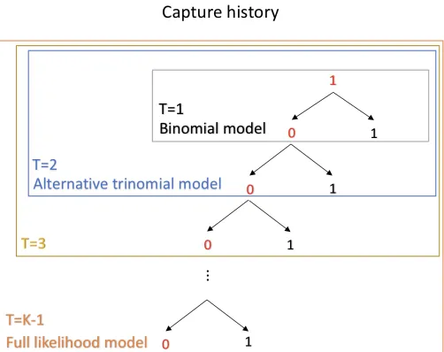
As a final possibility, Burchett (2017) developed an alternative model to address the

missing-covariate problem for open-population CR data by modifying the CJS likelihood to allow the

truncation of capture histories. A tuning parameter T ∈ {1,2, ...,K − 1} was introduced to determine the number of occasions to truncate the likelihood contribution after each capture or

recapture. The maximum value ofT isK−1 and all values ofT build a spectrum. Moreover, Burchett (2017) showed that the alternative model includes the binomial (T = 1) and full

likelihood models (T = K −1) as special case since they fall at the two ends of the spectrum. Assumptions of the alternative model are all the same as those of the full likelihood model

so that the mean rate changeµt between occasions and the rate of varianceσ2 are considered

and the likelihood function involves the contribution of the covariate values. I introduce the

alternative trinomial model (the case whenT = 2) in more details in the following paragraph.

Heuristically, the alternative trinomial model is constructed by considering three possible

events when an animal is captured and released on occasiont:

(1) It is recaptured on occasiont+1,

(2) It is not recaptured on occasiont+1 but is recaptured on occasiont+2, or

(3) It is not recaptured on occasionst+1 ort+2.

Note that the first event includes two capture occasions, which can be represented by the

(28)

capture occasions. Thus we need to define the new transition,πi,t(a,b,c|ppp, βββ,zizizi), which contains

three occasions, as:

πi,t(a,b,c|ppp, βββ,zizizi)= Pr(ωi,t+2 =c, ωi,t+1 =b|ωi,t =a,ppp, βββ,zizizi), a,b,c∈ {0,1}. (2.26)

Moreover, this model needs us to start with every capture so that all the transitions fromωi,r =0

will be omitted. In addition, if ωi,r+1 = 1 we will no longer take ωi,r+2 into consideration. That is, for the alternative model, we only consider three forms of transitions,πi,r(1,1|ppp, βββ,zizizi),

πi,r(1,0,0|ppp, βββ,zizizi), andπi,r(1,0,1|ppp, βββ,zizizi), whose expressions are:

πi,r(1,1|ppp, βββ,zizizi)= φi,rpr+1

πi,r(1,0,1|ppp, βββ,zizizi)=φi,r(1− pr+1)φi,r+1pr+2

πi,r(1,0,0|ppp, βββ,zizizi)=1−φi,rpr+1−φi,r(1− pr+1)φi,r+1pr+2.

(2.27)

For example, if individualihas capture history 0110010, the full likelihood is:

f(zi,4|zi,3)f(zi,5|zi,4)· f(zi,6|zi,5)· f(zi,7|zi,6).

(2.28)

After deleting transitions from 0, the truncated alternative trinomial likelihood is

f(zi,5|zi,4)· f(zi,6|zi,5)· f(zi,7|zi,6).

(2.29)

It is immediate thatφi,r+1inπi,r(1,0,1|ppp, βββ,zizizi) andπi,r(1,0,0|ppp, βββ,zizizi) cannot be computed due to

the missing covariatezi,r+1. Consequently, it is necessary to model the missing covariates using the drift model for the truncated likelihood of the alternative trinomial model. Once again, I

fit the alternative trinomial model in the Bayesian framework using JAGS to perform MCMC

(29)

2.4. AlternativeTrinomialModel 23

Similar to the alternative trinomial model, we can build more different models by changing

the value of T. For the model with T = m, when an individual was captured on occasion t

but not recaptured from occasiont+1 to t+m−1, mmore occasions are considered. If the individual was recaptured on occasionr(t+1≤ r≤ t+m−s), we truncate the transition on this occasion. In conclusion, every capture initializes a transition, which contains occasions from

this capture to the next but the maximum number of occasions contained in this transition is

m+1. Then the product of all the transitions and the densities of covariates give the truncated

likelihood. For example, whenT =3 for the alternative model, the truncated likelihood for the

capture history 011000110 is

(2.30)

where

πi,3(1,0,0,0|ppp, βββ,zizizi)= Pr(ωi,6= 0, ωi,5 =0, ωi,4 =0|ωi,3 = 1,ppp, βββ,zizizi). (2.31) Figure 2.1 illustrates the association between the binomial model, the full likelihood model, and

the alternative trinomial model. The likelihood contribution related to each release of a marked

individual is constructed by following the tree to a terminal node - either a recapture (1) or the

edge of the bounding box defined by the number of occasions considered after release. When

T is equal to K −1, the model is exactly the full likelihood model because once you cannot recapture an animal the entire capture history will be involved in the likelihood. If we do not

consider any occasion forward when encountering πi,r(1,0|ppp, βββ,zizizi), the model reduces to the

binomial model. In addition, the number of the missing covariates needed to be computed for

(30)

Figure 2.1: The structure of the alternative model.

2.5 Scaled Logit Link Function

The goal of my thesis is to see how these different models behave when the logit link function

relating survival to the covariate is replaced with a scaled logit function such that survival

probability is bounded in (0,c) for some 0 < c < 1. Under the logit link function the survival

probability tends to be one as zit increases to infinity if covariate coefficientβ1 is positive or as zit decreases to infinity if β1 is negative. However, it may not be realistic to assume that survival probabilities approach one in some situations. For example, if an individual’s weight

is the covariate of interest, then it may be reasonable to assume that an individual with a larger

weight has a higher survival probability, but it is unreasonable to assume that the individual

will undoubtedly survive from one occasion to the next when its weight is sufficiently large.

For this reason, we scale the logit link function using a specific valuec(0<c<1) such that

φ∗

(zi,t|βββ,c)= c

exp(β0+β1zi,t)

exp(β0+β1zi,t)+1

. (2.32)

(31)

2.5. ScaledLogitLinkFunction 25

As mentioned before, we consider the parameters in the model to be estimable if the

like-lihood provides strong information about the value of the parameters. In the case of MLE, we

consider the parameters to be estimable if there is a single, unique setting of the parameters

that maximize the likelihood. Contrary to this, the likelihood is non-estimable if we can find

at least two sets of parameters which generate the same maximum likelihood value. In our

specific situation, we actually find that there are infinitely many sets of parameters defined by

an interval I for the scalar parameter c such that for any c in this range we can find values of

the other parameters that maximize the likelihood. This is easily visualized as a flat spot in the

profile likelihood computed by fixing the value of c and then maximizing over the remaining

parameters.

For the Bayesian method, non-estimability implies two things: first, that the posterior

dis-tribution provides little information about the value of the parameter and second, that the shape

of the posterior distribution depends heavily on the choice of prior (a situation called prior

sensitivity). Consider a simple example in which there is only one parameter,θ, in the model.

The posterior distribution are beliefs about the value of the parameter given the observed data

and it is proportional toπ(θ)L(x|θ), where xrepresents the observed data. Hence, if the prior distribution ofθ is a constant, then the posterior distribution is proportional to the likelihood

L(x|θ) and has the same shape as the likelihood. Therefore, if the likelihood has a flat spot, as occurs in our case, then a flat spot will also appear on the posterior distribution,

lead-ing to the non-estimability of the parameter. Moreover, if the likelihood does not provide

strong information about the parameter then the posterior distribution will change

consider-ably when the prior is replaced by another distribution (e.g., if the uniform prior is replaced

by a beta prior with parameters α, β, defined on the interval [0,1]). In problems with

multi-ple parameters we can examine the estimability of one parameter by considering the marginal

posterior distribution of this parameter. In our case, the marginal posterior distribution of c

isπ(c|x) ∝ π(c)R_θ

−cL(x

|θ)π(θ−c)dθ−c, whereθrepresents the full set of parameters andθ−c the

(32)

and single parameter models are different, the properties of the non-estimable model like prior

sensitivity and non-estimability should not be changed. If the model is estimable, then the

posterior distribution should mainly depend on the likelihood rather than the prior distribution,

and should provide a reasonable estimate and credible interval for any sensible specification of

(33)

Chapter 3 Results

3.1 Binomial Model

3.1.1 Theoretical results

The key result for the binomial model is that parameters are not estimable when survival is

modeled via the scaled logit link function. This can be proved directly from the theoretical

analysis by showing that there is an alternative set of parameters that produce exactly the same

likelihood.

Theorem 3.1.1 For the bionomial model, where we assume the survival probabilityφ∗(zi,t|βββ,c)

is linked with the covariate zitthrough the scaled logit link function,

φ∗

(zi,t|βββ,c)= c

exp(β0+β1zi,t)

exp(β0+β1zi,t)+1

, (3.1)

we have

L(βββ,p,1;z)= L(βββ,p∗,c;z), for anymax

2≤r≤Kpr< c≤1, (3.2)

where p∗t = pt/c, t = 1, . . . ,K. More generally, for any values of the parametersβββ, ppp(1)(1)(1) and

(34)

any pair c(1),c(2) ∈

max 2≤r≤Kpr,1

, we can find another set of parametersβββ, ppp(2)(2)(2)such that

L(βββ,p(1),c(1);z)=L(βββ,p(2),c(2);z). (3.3)

Hence, the binomial model is not estimable under the scaled link function.

Proof Recall from Section 2.1 that the likelihood for the binomial model using the logit link

ignores all transitions starting from 0. Hence, there are only two kinds of transitions left, which

are

∗

(zi,r|βββ,1)pr+1.

(3.4)

Under the scaled logit link function (3.1), these two transitions can be written as:

πi,r(1,0|ppp, βββ,1) = 1−φ∗(zi,r|βββ,1)pr+1 = 1− exp(β0+β1zi,t)

exp(β0+β1zi,t)+1 pr₊1

= 1−c exp(β0+β1zi,t)

c

= 1−φ∗(zi,r|βββ,c)p∗r+1

= πi,r(1,0|ppp∗∗∗, βββ,c) (3.5)

πi,r(1,1|ppp, βββ,1) = φ

∗

(zi,r|βββ,1)pr+1 = exp(β0+β1zi,t)

= c exp(β0+β1zi,t)

c

= φ∗

(zi,r|βββ,c)p

∗

r+1 = πi,r(1,1|pp∗

∗

(35)

3.1. BinomialModel 29

From equation (3.5), we can see thatπi,r(1,0|ppp, βββ,1) = πi,r(1,0|ppp∗∗∗, βββ,c) andπi,r(1,1|ppp, βββ,1) =

πi,r(1,1|ppp∗∗∗, βββ,c). Hence, the partial likelihoodsL(βββ,p,1;z) andL(βββ,p∗,c;z) which are defined

by equation (2.8) and constructed by πi,r(1,b|ppp, βββ,1) and πi,r(1,b|ppp∗∗∗, βββ,c) are also the same.

Moreover, the capture probability should lie between 0 and 1, so ppp/c is required to be less

than 1 (i.e., max2≤r≤K pr <c<1). Note that the likelihood is conditional on the first capture

thus p1is not involved in the likelihood. Therefore, all parametersp∗r = ppp/candβββ,cwherec∈

max 2≤r≤Kpr,1

result in the same likelihood. More generally, for any set of parameters (β,β,β,ppp(1)(1)(1),c(1)) or (β,β,β,ppp(2)(2)(2),c(2)) both satisfying the relatinships in equation (3.5), we have

L(βββ,p(1),c(1);z)= L(βββ,p,1;z)= L(βββ,p(2),c(2);z).

Hence, the binomial model is not estimable under the scaled logit link function.

3.1.2 Analysis of a simulated data set

To numerically confirm the Theorem 3.1.1, I conducted the analysis of a single simulated data

set. I simulated a CR data set for a total ofn = 500 individuals over K = 6 capture occasions

using the following setting of parameters:

β0 =2, β1 = 2

c=0.8

p=0.8

(µ1, µ2, µ3, µ4, µ5)= (0,0,0,0,0) σ=0.1

µ0 =0, σ0 =1

(3.6)

where I assume the capture probability p is the same on all occasions for simplicity of

(36)

distribution of mean µ0 and variance σ20, and then used the mean rate vector µµµ and variance σ2 _{to generate 500 individual covariate vectors with length} _K_{. For each individual, the}

sur-vival probabilities were computed for the first K−1 covariate values, givenβ0andβ1. Then I sampledDiwhich was the last occasion before the individual died. Finally, the capture history

for each individual was generated based on the capture probability pbut if the individual died

before occasion K then the capture history from the death occasion to occasion K was set as

0. Then the binomial model was fit to the data repeatedly with values of fixed c. That is, I

fixed the value ofcfirst, and then maximized the likelihood function to get MLEs of the other

parameters including p,β0, andβ1.

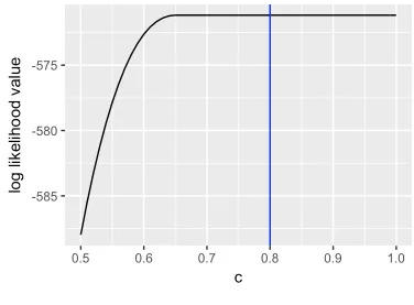
The analysis of this simulated data set exactly reproduced what we expected based on

the theoretical results. In Figure 3.1, when c increases from 0.5 to 0.65, the maximum

log-likelihood under fixedcincreases and then remains unchanged at the maximum value (-571.173).

The appearence of the flat spot confirms that the binomial model is not estimable under the

scaled link function because all c’s and other corresponding parameters in the flat spot can

generate the same maximum likelihood value.

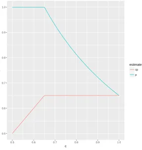
The appearance of the growth of the log likelihood value at the beginning is due to the

truncation of parameters and Figure 3.2 explains the phenomenon in a more visual way. The

blue curve illustrates how the estimate of p varies with the change of c while the red curve

describes the product of ˆpandc. Let ˆp(1) denote the estimate ofpunder the logit link function.

From the theoretical analysis, we know that ˆp is related to c (i.e., p(c)), and is equal to the

ˆ

p(1)/cfor ˆp(1)< c< 1. The red curve confirms this result since ˆp(1)=0.65 and ˆp(c) remains

a constant from c = 0.65 to 1. Therefore, when c ≤ pˆ(1), ˆp(c) = pˆ(1)/c > 1, so ˆp(c) is truncated at 1. This means that the profile likelihood is below the maximum whenc < 0.65,

(37)

3.2. TrinomialModel 31

Figure 3.1: The log-likelihood value of the Binomial model under the scaled link function with the scalarc. The black line is the profile log-likelihood value as a function ofcfor the Binomial model. The blue line is the true value ofc(c=0.8).

3.2 Trinomial Model

The complexity of the trinomial model makes it difficult to explore the estimability

mathemati-cally, and so we only examine the model by simulation. I simulated a new data set (MRR data)

for a total ofn= 500 individuals over K = 6 occasions using the same parameter values as in

the above simulation but adding a constant recovery probabilityλ=0.4. Also, we assume that

the capture probability pand the recovery probabilityλare the same on all occasions for ease

of implementation. Then the trinomial model was fit to the data repeatedly with values of fixed

clike we did in the binomial model. Then this model was fit to the data again butcserved as a

parameter to be estimated.

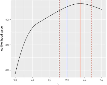
The analysis of the simulated data in this case showed that the trinomial model is estimable,

which can be seen in Figure 3.3. The black line in Figure 3.3 shows how the maximum

log-likelihood value changes as the value ofcchanges. The solid vertical red line (ˆc=0.88) is

(38)

Figure 3.2: The estimates of capture probability pof the Binomial model under the scaled link function with the scalarc. The blue line is the estimate ofpas a function ofcfor the Binomial model. The red line is the product of the estimate of pandc.

0.5 0.6 0.7 0.8 0.9 1.0

c

p

estimate

cp p

two dashed lines indicate the 95% confidence interval (0.76 0.94) of ˆc. Whencrises from 0.5

to 0.88, the log-likelihood value increases from -821.51 to−793.65. Then the log-likelihood value decreases ascincreases from 0.88 to 1. The biggest value among all log-likelihood

val-ues is -793.65 and the corresponding fixedcis 0.88, exactly equal to the maximum likelihood

estimate ˆcwhencis treated as an unknown parameter to be estimated. That is to say, ˆcis the

only value of c that generates the maximum likelihood value. Hence, the trinomial model is

estimable under the scaled link function.

3.3 Alternative Trinomial Model and Full Likelihood Model

One challenge with the trinomial model is that it requires the recovery of dead individuals,

(39)

es-3.3. AlternativeTrinomialModel andFullLikelihoodModel 33

Figure 3.3: The log-likelihood value of the Trinomial model under the scaled link function with the scalarc. The black line is the profile log-likelihood value as a function of c for the Trinomial model. The blue line is the true value ofc(c=0.8). The red solid line is the mle of

c. The two dashed red lines indicates the 95% confidence interval of ˆc.

timable. In this section, the estimability of the binomial model, the alternative trinomial model,

and the full likelihood model are analyzed through Bayesian inference. As with the trinomial

model, we can only assess the estimability of the alternative model by the simulation study due

to the complexity of the likelihood. Three models: the binomial model, the alternative

trino-mial model, and the full likelihood model were fit to the data wherecis an unknown parameter

to be estimated through the Bayesian inference implemented by MCMC sampling. Following

the same setting of parameters used for the simulation under the binomial model, we simulated

a data set for a total ofn = 500 individuals over K = 6 capture occasions. For each model, in

(40)

10000 and 100000, respectively. The prior distributions of all parameters are set as folllows:

c∼U[0,1]

p∼ U[0,1]

µt ∼ N(0,1002)

σ=1/τ, τ∼Gamma(0.001,0.001), t =1, ...,K−1 β0 ∼ N(0,102)

β1 ∼ N(0,102).

(3.7)

Then the posterior distributions ofcunder the three models can be obtained, from which I can

assess the estimability.

As expected, the posterior distributions of c show the estimability of three models. The

appearance of the flat spot of the binomial model under the scaled link illustrates the posterior

distribution provides limited information about the parameter when the prior is uniform which

is consistent with the result of the non-estimable model discussed in Section 2.5. In contrast,

based on Figure 3.4 we can see from the posterior distributions of the alternative trinomial

model and the full likelihood model that c is highly likely to be in the interval (0.75,0.82)

because 99% mass of the distributions lies below 0.82 and above 0.75. Hence, these explain

the binomial model is not estimable while the alternative trinomial and the full likelihood model

are estimable under the scaled logit link.

Compared with the full likelihood model, the alternative trinomial model has less runtime,

and can estimatecaccurately since the point estimate ofcis 0.78 and the 95% interval estimate

is (0.76,0.80). The point estimate ofcof the full likelihood model is 0.79 and the 95% interval

(41)

3.4. PriorSensitivity 35

Figure 3.4: Posterior density ofcfor three models based on Bayesian inference. The black line is the true value ofc(c=0.8).

0 10 20 30

0.6 0.7 0.8 0.9 1.0

c

P

oster

ior Density of c

Model

alternative trinomial model binomial model full likelihood model

3.4 Prior Sensitivity

Another way to illustrate the non-estimability of the binomial model is to consider prior

sen-sitivity in a Bayesian framework. The non-estimable model is sensitive to the change of the

prior distribution according to our analysis in Section 2.5. To show this, I continued to use the

data set in the last section and parameter settings but changed the prior distribution ofcto the

Beta distribution. Then I ran the binomial model, the alternative trinomial model, and the full

likelihood model using three different priors, Beta(2,3), Beta(2,8) and Beta(2,18). Figure 3.5

combines the results from Beta priors and the result from the uniform prior, which is actually

a Beta distribution with parametersα = β = 1, indicating the prior sensitivity of the binomial

model.

(42)

dramatically while that of an estimable model is almost unchanged. In Figure 3.5, when the

second parameterβ is larger, the posterior density curve ofc for the Binomial model is

thin-ner and higher, consistent with the characteristics of the beta distribution. However, for the

alternative trinomial and full likelihood models, the posterior density curves change very little

although the prior distribution of care changed a lot. So we still can determine the estimate

ofc. This further indicates that the binomial model with the scaled logit link cannot be used

reliably in practice.

Figure 3.5: Posterior density ofcof different prior distributions for three models: the binomial model (A), the alternative trinomial model (B), and the full likelihood model (C). The black line is the true value ofc(c= 0.8).

0 10 20 30 40

0.5 0.6 0.7 0.8 0.9 1.0

c

P

oster

ior Density of c

A

0 10 20 30 40

0.5 0.6 0.7 0.8 0.9 1.0

c

B

0 10 20 30 40

0.5 0.6 0.7 0.8 0.9 1.0

c

P

oster

ior Density of c

Prior

(43)

Chapter 4 Conclusion

In this thesis, I have investigated the estimability of the binomial model, trinomial model,

alternative trinomial model, and the full likelihood model when the scaled logit link function

is used for estimating population parameters with individual, continuous, and time-dependent

covariate. The estimability of models can be checked under the frequentist (MLE) and the

Bayesian paradigm. The likelihood of the binomial model is simple to construct and so I have

mathematically investigated the behaviour of the MLE for this model. Since the standard MLE

technique does not work for the models with unknown covariates, i.e., the alternative trinomial

and full likelihood models, I consider a Bayesian approach for these models. In addition,

one may be curious about the difference between the estimability and the identifiability. The

distinction between identifiability and estimability is essentially determined by whether or not

a parameter can never be estimated or can be estimated for some data sets but not others.

Non-identifiability says that there are different combinations of the parameters that produce

the same distribution of the data (i.e., f(x|θ)). Note that there is nothing about the observed data in this statement. For the estimability, on the other hand, it depends on the configuration

of the data. In MLE, it occurs when there are different values of the parameters that produce

the same maximum likelihood for the specific data that is observed. In Bayesian framework,

non-identifiability occurs when the posterior distribution cannot provide strong information

(44)

about the value of parameters and is sensitive to the change of the prior distribution. The

binomial model and the trinomial model use the reduced likelihood not the full likelihood, and

thus have nothing to do with the identifiability. The alternative trinomial model and the full

likelihood model are implemented in the Bayesian framework where a sample is obtained from

the posterior distribution π(θ|x) of the parameters and a density plot of the sample is made to see how parameters of interest are distributed along with the domain of definition. That is, the

posterior distribution π(θ|x) only determine whether or not the estimate can be estimated and we cannot conclude anything about the likelihood. Therefore, I explore the estimability of the

four models, not the identifiability.

The non-estimability of the binomial model under the scaled logit link function is proved

by theoretical analysis and confirmed through the simulation analysis. Theorem 3.1.1 shows

that the reduced binomial likelihood values generated by two different sets of parameters are

equal, indicating the non-estimability of the binomial model. As for the simulation analysis,

the non-estimability behaves as the curve of the profile likelihood value at different fixed scaler

c has a flat spot, which is consistent with the result of the theoretical analysis. Moreover,

the binomial model is sensitive to the prior distribution, which is an important characteristic

of non-estimable models under the Bayesian framework. When the prior distribution of c

changes, significant changes have taken place in the shape of the posterior distribution. It is

very noteworthy that when the prior distribution ofcis the uniform distribution on [0,1], the

posterior distribution ofc also has a flat spot resulting in the parameters cannot be estimated

and we cannot ascertain the location of the true parameter in the wide region of the parameters.

The trinomial model is still estimable when the scaled logit link function is used, which

can be seen from the curve of the likelihood value at different values ofc. The likelihood value

on the curve increases untilcreaches the estimate ofcand then decreases. This indicates that,

no other set of parameters can generate the same likelihood as the set of true parameters, thus

the model remains estimable under the scaled logit link function.

Exploring the Estimability of Mark-Recapture Models with Individual, Time-Varying Covariates using the Scaled Logit Link Function

Scholarship@Western

Scholarship@Western

Exploring the Estimability of Mark-Recapture Models with

Exploring the Estimability of Mark-Recapture Models with

Individual, Time-Varying Covariates using the Scaled Logit Link

Individual, Time-Varying Covariates using the Scaled Logit Link

Function

Function

Summary

Contents

List of Figures

Introduction

1.1

Overview

1.2

Closed-Population Models

1.3

Open-Population Models

1.4

CJS Model with Covariates

Methodology

2.1

Binomial Model

2.2

Trinomial Model

2.3

Full Likelihood Model

2.4

Alternative Trinomial Model

2.5

Scaled Logit Link Function

Chapter 3

Results

3.1

Binomial Model

3.1.1

Theoretical results

3.1.2

Analysis of a simulated data set

3.2

Trinomial Model

3.3

Alternative Trinomial Model and Full Likelihood Model

3.4

Prior Sensitivity

Chapter 4

Conclusion