Inversion of an Inductive Loss Convolution Integral for Conductivity Imaging

Inversion of an Inductive Loss Convolution Integral

for Conductivity Imaging

Joe R. Feldkamp*

Abstract—Electrical conductivity imaging in the human body is usually pursued by either electrical impedance tomography or magnetic induction tomography (MIT). In the latter case, multiple coils are almost always used, while nonlinear reconstruction is preferred. Recent work has shown that single-coil, scanning MIT is feasible through an analytical 3D convolution integral that relates measured coil loss to anarbitrary conductivity distribution. Because this relationship is linear, image reconstruction may proceed by any number of linear methods. Here, a direct method is developed that combines several strategies that are particularly well suited for inverting the convolution integral. These include use of a diagonal regularization matrix that leverages kernel behavior; transformation of the minimization problem to standard form, avoiding the need for generalized singular value decomposition (SVD); centering the quadratic penalty norm on the uniform solution that best explains loss data; use of KKT multipliers to enforce non-negativity and manage the rather small active set; and, assignment of the global regularization parameter via the discrepancy principle. The entire process is efficient, requiring only one SVD, and provides ample controls to promote proper localization of structural features. Two virtual phantoms were created to test the algorithm on systems comprised of ∼ 11,000 degrees of freedom.

1. INTRODUCTION

Electrical conductivity is a property that varies considerably throughout the human body [1]. Thus, an ability to image its spatial variability could be useful from a diagnostic standpoint. Various disease states may cause the conductivity to differ from that exhibited in normal tissue [2, 3]; or, the appearance of growths and other obstructions [4] could alter the way that induced electrical currents behave so that the obstruction becomes visible. Two methods for producing these images in medical applications have appeared over the past few decades — one of them electrical impedance tomography [5], and the other, magnetic induction tomography [6] (MIT). The latter approach offers the considerable advantage of being non-contact as well as noninvasive. Nearly all MIT research has been based upon a multiple coil system placed in the vicinity of the conductive target. One coil functions as a source that interacts with the target, while any other functions as a detector, responding both to the primary field as well as the perturbation of the field due to the target’s presence. This multi-coil approach is inherently nonlinear, involving a forward problem that must numerically solve Maxwell’s equations prior to image reconstruction — and do so for each position of the coil array. Given that the forward problem is nonlinear, it has been stated that nonlinear image reconstruction is a necessity in order to achieve satisfactory results [7].

More recently, an alternate approach has been evaluated that requires the use of only one coil [8, 9], whose interaction with nearby conductive objects is manifested as an inductive loss, resulting from the secondary field generated by induced eddy currents [10]. The coil under consideration consists of closely-spaced parallel layers of concentric circular loops, all connected in series. Since electrical conductivity is

Received 14 February 2017, Accepted 1 April 2017, Scheduled 12 April 2017

quite low in biological targets (5 S/m), rather high excitation frequencies (∼10 MHz) are needed in order to produce a measurable loss in such coils (∼1 ohm) and still maintain high signal to noise ratio. To leverage the usefulness of measured coil loss information, an analytical model was developed that expresses alinear relationship between inductive loss in coils consisting of circular loops and anarbitrary

electrical conductivity distribution. The key assumptions behind the model are that permeability and permittivity are spatially uniform; conductivity is small (10 S/m); excitation frequency is sufficiently low that quasi-static field conditions hold; and, that spacing between coil loops residing in different planes is sufficiently small that they essentially share a common plane. The model has been validated numerous times experimentally [8, 9, 11], showing that it is indeed quantitative when permittivity is uniform, and that linearity is preserved even when permittivity shows large sudden spatial variation beyond what is present in biological systems. Furthermore, the analytical model is easily written as a 3D convolution integral that does not require calibration, facilitating its use for image reconstruction.

Because there is just one coil, a scan operation is needed that repeatedly relocates the coil in the vicinity of the target such that the EM field of the coil can intercept the target in a large number of non-redundant ways. With inductive loss written as a convolution integral that convolves the electrical conductivity distribution with a sampling function (kernel), a sufficiently detailed scan should contain adequate information to enable computation of the desired electrical conductivity distribution. The advantages of this approach include reduced hardware complexity, since only one coil has to be managed; and, given the fact that the convolution integral shows a linear relationship between loss and the full conductivity distribution, image reconstruction is made easier.

Nevertheless, image reconstruction has remained challenging, mostly because of the rapid decay of the EM field in a coil’s vicinity. But this is also true of coils used in any form of MIT and appears as a similar challenge in other forms of tomography, such as diffuse optical tomography where light scattering greatly attenuates the propagation of light into and out of a sample medium [12]. In our previous work with single coils, inversion proceeded by first discretizing the convolution integral on a finite element mesh that spans the space of the conductive target, so that coil loss b can be predicted through a simple matrix operation acting on the unknown conductivity vector x: b ≈A˜x. Most commonly, the number of measurements is far smaller than the number of unknowns, necessitating the use of regularized least squares analysis. A solution was pursued by Tikhonov regularization that increasingly penalized those solutions having higher gradient norms. The usual “normal” equations were developed and then passed to an open source solver that imposed non-negativity on the solution via an active set approach developed by Haskell and Hanson [13]. An optimal value for the regularization parameter was chosen using an L-curve technique. Not only was the process inefficient, solutions showed excessive smoothing and were prone to misplace structural features in those circumstances where coil loss measurements were restricted to locations close to a target — both issues were found to be aggravated by instrumental noise.

2. SVD NNLS APPLIED TO MIT CONVOLUTION INTEGRAL

The discretized convolution integral (next section) leads to a prediction of coil loss measurements from a conductivity vector x consisting of n conductivity values on a finite element (FE) mesh. For the application to single-coil MIT, coil loss measurementsbare obtained atm scan positions in the vicinity of a conductive target. Coil loss prediction is given by the vector ˜Ax, where the matrix ˜A ism×nand consists of components that are determined according to coil position and orientation. Measurements are expected to be few in number, such that m < n, giving an underdetermined system.

Because conductivity is non-negative, we require thatx_i ≥0 for each i. Since scanning inevitably produces many similar measurements, the matrix ˜A is expected to be ill-conditioned (large condition number). Thus, we attempt to find the best conductivity by minimizing a penalized 2-norm, subject to non-negativity:

min1 2

_A˜_x−b2

2+

1 2τ

2_D˜x−β2

2 s.t. x≥0 (1)

Problem in Equation (1) is made more flexible, without requiring additional computational effort, by permitting each node to be penalized independently of the others. This is accomplished via the invertible, diagonal regularization matrix ˜D, with diagonal entries d_j > 0. In order for the weights in the diagonal matrix to produce some benefit to the solution process, guidance on selection of the components of ˜D is essential — we return to this issue later. For now, we mention that the model might inherently weight some members of the solution set more so than others, so that ˜D offers an opportunity to compensate. Furthermore, if some solution members tend to contribute very little to a predictedb_i, or should have little impact on the error norm (first term of Equation (1)), then these could be penalized heavily to ensure a givenx_i remains well inside an expected interval through appropriate assignment of β_j and d_j.

Commonly,β= 0, but here we take advantage of the fact that the solution will typically lie within some interval 0≤x_i 5 S/m rather than an unbounded domain. For example, electrical conductivity within human tissues [1] is usually less than ∼ 5 S/m, suggesting that β ought to be set somewhere inside this expected interval — leading to a “shifted penalty”, as we characterize it here. Thus, the regularization term not only promotes a well-conditioned problem with a unique solution [14], but leads to a greater penalty when x_i = β_i. If the regularization parameter τ is made large compared to the largest singular values of ˜A, then solutions tend to be heavily localized around β [15]. Thus, β is set

>0 so that the number of negative x_i values is reduced when constraints are absent, whileτ is set to a non-zero value within the range of the singular values associated with ˜A. Non-negativity is addressed using an active set method, but is made more efficient as a result of the shifted penalty, which tends to reduce the number of needed constraints, and thus the size of the active set. We proceed with these definitions to transform minimization problem in Equation (1) into standard form:

z= ˜Dx ; ζ= ˜D β (2)

Minimization problem in Equation (1) becomes:

min1 2

_A˜_D˜−1_z−b2 2+

1 2τ

2_z−ζ2

2 s.t. z≥0 (3)

Except for the shifted penalty, problem in Equation (3) is now in standard form [16], showing how matrix ˜A is actually pre-processed by ˜D−1, which is meant to balance the role of each component of the solution, provided there is some meaningful approach to accomplishing that. As long as the computational cost is acceptable, getting to standard form is also feasible using square regularization matrices other than ˜D, provided they are not singular [17]. The primary benefit of getting to standard form, initially proposed by Eld´en [18], is improved solution efficiency.

SVD† is now applied to the matrix product appearing in Equation (3), as follows:

˜

AD˜−1 = ˜US˜V˜T (4)

Orthogonal matrices and singular values are modified due to the pre-multiplication of ˜A by the inverse of ˜D with the intention that solution components have a more equitable chance to contribute to the measurement vector in a noisy environment. To continue our development, we make the additional assignments:

z= ˜V y; b= ˜Ub; ζ = ˜V β (5)

Substitution of Equation (5) into Equation (3) leads to a form for the minimization problem especially suitable for our MIT inversion problem since it is readily amenable to straightforward algebraic solution:

min1 2

_S˜_y−b2

2+

1 2τ

2_y−β2

2 s.t. x or z≥0 (6)

After expanding the convex objective function in Equation (6) and adding non-negativity constraints for some select members of the solution set, {x_l(k);k= 1,2, . . . , K}, i.e., the active set, we have the

Lagrange objective function:

L

y, λ

= 1 2 r i=1

s_iy_i−b_i2+1 2

m

i=r+1

b_i2+1 2τ 2 n i=1

y_i−β_i2+

K

k=1

λ_kx_l(k) (7)

Here, we assume that r ≤ m < n, where the matrix ˜A has rank r; when r = m (usually), the second term on the right side is absent. Constraints, enforced via the KKT multipliers{λ_k}, are only applied to those{x_l(k)}belonging to the active set — note the mapping implied by the subscript that identifies

the correct solution component index associated with the kth constraint. To establish an initial active set, L(y, λ) is first minimized without constraints while β is chosen to deliberately reduce the size of the active set. Nodes with negative conductivity values are identified and placed into the active set for the first iteration following initialization. At each new iteration, KKT multipliers are examined, so that a constraint is released when positive, but maintained when negative. Of course, those nodes not in the active set continue to be examined and placed into the active set if their values are found to be negative.

Optimality equations are written for each of the unknowns in Equation (7), which requires that we set the partial derivative ofL with respect to each of they_j to zero. These may be solved for the{y_j}

in terms of the KKT multipliers:

y_j = ⎧ ⎪ ⎪ ⎪ ⎪ ⎪ ⎪ ⎪ ⎪ ⎪ ⎨ ⎪ ⎪ ⎪ ⎪ ⎪ ⎪ ⎪ ⎪ ⎪ ⎩

s_jb_j+τ2_β

j− K

k=1

λ_kV_l(k)j/d_l(k)

s2_j +τ2 ; j ≤r

τ2_β

j− K

k=1

λ_kV_l(k)j/d_k

τ2 ; r < j≤n

; k→l mapping (8)

The complementarity conditions, which directly enforce non-negativity on members belonging to the active set, are simpler:

x_l(q) =

n

j=1

V_l(q)j

d_l(q) yj = 0; q→l mapping implied (9)

Substitution of Equations (8) into Equation (9) allows us to obtain the KKT multipliers from a relatively small set of linear equations:

K

k=1

P_qkλ_k=

n

j=1

V_l(q)j

d_l(q)

y_j0; q= 1,2, . . . , K(∼1500)n(∼11,000) (10)

The elements for the symmetric matrix,P_qk, are:

P_qk= 1

d_l(q)dl(k)

n

j=1

V_l(q)jVl(k)j

The vector components ofy0are just the unconstrained solution, obtained by setting all KKT multipliers to zero in Equation (8). Equation (10) is solved using an LDLT decomposition method, and is kept smaller in size ifβ is chosen within the expected solution interval and the regularization parameterτ is kept nearer to the larger singular values in the set {s_j}. By choosingτ nearer the middle of the set of singular values, the current solution approach behaves similarly to a truncated SVD method [15] since those singular values which are much smaller than τ have little or no effect on the solution (filtering) — note that all singular values are used here and regularization is controlled by choice ofτ rather than truncation. Since the active set may change “membership” with each iteration, matrix ˜P has to be recomputed, but only for those components new to the active set.

Subsequent to solving Equation (10), the KKT multipliers are returned to Equation (8) to get the new solution (either z orx). At that point, both the new solution and KKT multipliers are examined in order to establish a new active set for the next iteration. Though not following the same active set method developed by Haskell and Hanson [13], which adds or drops only one constraint per iteration, we expect similar behavior — i.e., convergence in a finite number of steps [[19], p. 114]. In fact, for the MIT application we consider in the next section, convergence is typically obtained after 5 to 7 iterations — determined by the attainment of a stable active set, with KKT conditions satisfied.

This algorithm requires a choice forβ, which establishes a location where the penalty term is zero — optionally, individual components of the penalty may be forced to zero at customized locations, without requiring that the full penalty term is zero at a common location. Though many approaches to setting this vector are worth investigating, here we choose a uniform solution to Equation (1) with penalty term dropped. This sets all solution components to an identical value,β0, which is easily found

by minimizing the error residual with respect to β0:

β0=

m

i=1

b_i n

j=1

A_ij

m

i=1

⎛ ⎝n

j=1

A_ij

⎞ ⎠

2 (12)

For our MIT application, β0 becomes the conductivity of a target treated as having no structure, but

rather characterized by uniform conductivity. Certainly, it is possible to consider modifications toβ as the iteration process continues — for example, using a previous solution, or even an average of two prior solutions, with the idea that the next solution in the sequence is more penalized as it departs further from a prior solution [20, 21]. This is not explored here — we just use Equation (12) as a “zero order”, uniform solution.

To complete the algorithm, a value for the global regularization parameterτ is needed. This value is chosen using the so-called discrepancy principle [17], which requires that some reasonable estimate is available for the error associated with the measurement vectorb:

b−b_true≈ε (13)

Since this is something that we have measured for our application as the technology has progressed, the erroris available. Thus, the regularization parameterτ is decreased along a sequence tracking the singular values arising from the SVD of Equation (4), usually jumping several singular values at a time, until the following condition is approximately met:

_A˜_{x−b≈ε (14)}

becomes very small (much smaller than what is currently available via experiment), the solution step for KKT multipliers may become burdensome.

3. 3D CONVOLUTION FOR SINGLE-COIL, SCANNING MIT

Previously [8, 9], we have shown that the lossδZ in a planar coil consisting of circular concentric loops of wire is related to the electrical conductivity distribution of the target placed in the vicinity of the coil by:

δZ = μ

2_ω2

4π2

j,k √_ρ

jρk

d3xσ(r)

ρ Q1/2(ηj)Q1/2(ηk) (15)

Arguments for the circularly symmetric toroid (or ring) functionQ_1/2 lie in the interval 1< η <∞and are related to field position by:

η_j = ρ

2_+ρ2

j +z2c

2ρρ_j ; ηk=

ρ2+ρ2_k+z_c2

2ρρ_k (16)

Using any suitable fixed laboratory coordinate system, other symbols in Equations (15) and (16) are defined by:

σ(r): Electrical conductivity (real part) at field position: r=x, y, z,

ρ_k: Cylindrical radial distance from coil axis to wire loop ‘k’,

ρ: Cylindrical radial distance from coil axis to field point,

z_c: Perpendicular distance from coil plane to field point,

μ: Magnetic permeability — considered uniform,

ω: Angular frequency.

Assumptions leading up to Equation (15) have been discussed in earlier work. Equation (15), which we have called a mapping equation since it relates a coil loss measurement at a particular coil position and orientation to an entire electrical conductivity distribution, is actually a 3D convolution. This is made clear by recasting Equation (15) into the frame of the coil center — with the coil’s Z-axis perpendicular to the coil plane, while the coil’sX-axis andY-axis lie within the coil plane. Letting the vectorclocate the coil center relative to the lab frame origin, and the vectorr_c locate the field point in the coordinate system (CS) of the coil, we have the revised form for Equation (15):

δZ(c) =

σ_l

c+ ˜Rr_c

G(r_c)dx_cdy_cdz_c =

σ_l(r)G

˜

RT(r−c)

dxdydz (17)

A subscript, designating “lab”, has been attached to the conductivity as a reminder that the argument still evaluates to a vector in the lab frame, with the orthogonal rotation matrix ˜R mapping the vector

r_c from coil frame to lab frame. While arriving at Equation (17), we have made use of the fact that the determinant of the Jacobian transformation matrix is unity. In Equation (17), we have also made use of the definition:

G(r_c) = μ

2_ω2

4ρπ2

j,k √

ρ_jρ_kQ1/2(ηj)Q1/2(ηk) (18)

The function G(r_c) is recognized as the kernel of the convolution integral and is rapidly evaluated through use of a hypergeometric series for the toroidal functions [22] — the two forms in Equation (17) are equivalent, though the second is used here. Note that if the coil does not rotate relative to the lab frame as it is moved around, then the rotation matrix is just the identity matrix.

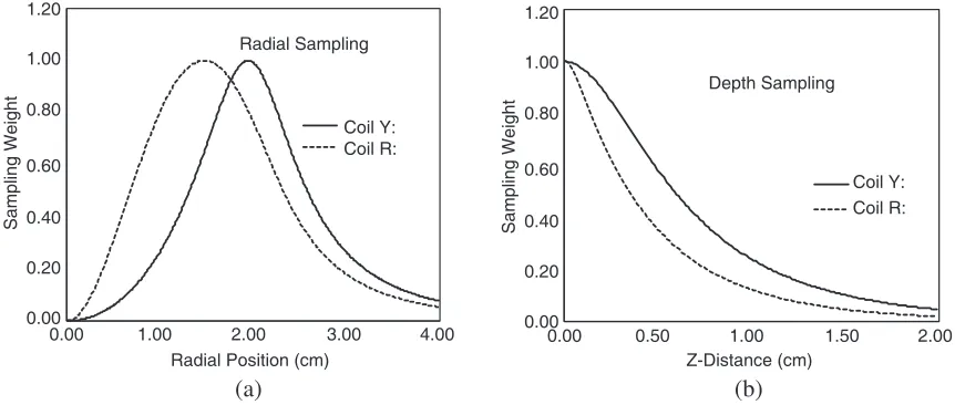
4. SETTING “WEIGHTS” IN REGULARIZATION MATRIX ˜D

As mentioned, the diagonal matrix ˜Dprovides an opportunity to selectively penalize contributions from individual solution components, and single coil MIT gives us an excellent example of how this can be used to our advantage. Its use here is motivated by successful application of a position-dependent regularization in diffuse optical tomography [12]. Essentially, the kernel function in the convolution integral naturally weights regions of space according to their contribution to the measured coil loss. Thus, plots of the kernel function, either along the coil’sZ-axis or radial axis are helpful in guiding how the components of ˜D are chosen. Here, kernel function plots (or sampling function) are given for two different coil designs to illustrate how “sampling” of space is dependent on coil geometry. The first, coil ‘R’, consists of five circular concentric loops in each of two layers (ten total) — spacing is 0.5 mm, so that all loops are considered to effectively lie in the same plane. The loops have radii of 4, 8, 12, 16 and 20 mm. Coil ‘R’ inductance was shown previously to be 2.155µH, and is used in all calculations for this work. A second coil ‘Y’ consists of 4 layers of loops, all set at a radius of 20 mm, with a spacing of

∼0.3 mm between layers — again, spacing is considered to be sufficiently small that they are considered to be in the same plane. Coil ‘Y’ inductance is easily computed to be ∼ 1.8µH (used here only for comparison purposes; a later publication will consider coil Y).

In a plane parallel to either coil, located at a distance of 5 mm from the coil plane, the kernel function is plotted as a function of radial distance from the coil axis in Figure 1(a). Note that coil ‘R’ gives a broader or smoother sampling of space while coil ‘Y’ tends to be more focused. However, in either case, since a coil scan primarily moves the coil in the plane of the coil and with minimal rotation, good sampling of space is achieved by collecting coil loss values on an appropriate lattice of points nominally parallel to the target (e.g., Latin Hypercube). It is likely that coil ‘Y’ would benefit from more data collection given its “tighter” sampling field. If in-plane sampling provides good “coverage”, which is reasonable in the absence of any obstructions that would inhibit such scanning, there is likely no particular reason to base weights upon these plots.

The situation is different for out-of-plane sampling during a scan. Obviously, the coil cannot be located inside the target to collect data, so it is imperative to understand how the kernel function varies with distance, normal to the coil plane. This is shown in Figure 1(b).

Regardless of coil type, the decay with Z-distance in Figure 1(b) is nearly exponential, except in the immediate vicinity of the coil plane. Figure 1(b) indicates that greater weight or importance is given to those points nearest to the coil plane, giving them an advantage in a noisy environment, so

1.20

1.00

0.80

0.60

0.40

0.20

0.00

Sampling Weight

Radial Sampling

Coil Y: Coil R:

0.00 1.00 2.00 3.00 4.00

Radial Position (cm)

1.20

1.00

0.80

0.60

0.40

0.20

0.00

Sampling Weight

Depth Sampling

Coil Y: Coil R:

0.00 0.50 1.00 1.50 2.00

Z-Distance (cm)

(a) (b)

that the solution from any inversion scheme will tend to favor points closest to the coil plane if nothing is done to relieve the bias. A simple procedure to help mitigate the bias applies an exponential decrease of the regularization weights in ˜Das solution components become associated with points farther from the coil plane, or target boundary:

d_j = exp (−ηz_j/zmax) (19)

Finite element mesh thickness is given as zmax, while zj is distance from target boundary to node

location, andη is a decay parameter meant to control the extent of bias mitigation. The other option is to directly use the curves shown in Figure 1(b), though distance-scaled to some extent. Both are tested here.

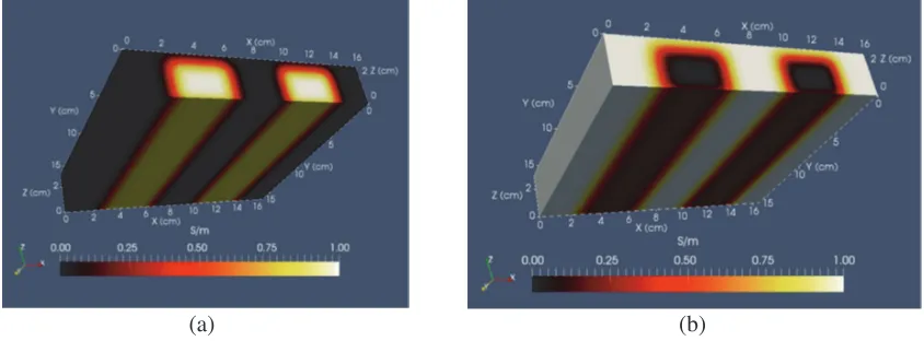
5. TARGET MIT PHANTOMS

Two virtual phantoms are used for algorithm testing under conditions that adjust regularization and noise. Phantoms consist of buried thick strips of altered conductivity — one with low conductivity strips (∼0.0 S/m) immersed in a higher conductivity matrix (∼1.0 S/m); a second with higher conductivity strips immersed in a lower conductivity matrix. In the first, two thick strips of very low conductivity material, embedded in background material of 1.0 S/m, are located within a 16.5 cm×16.5 cm×3.0 cm slab phantom as shown in Figure 2 — these low-conductivity strips are defined by regions having conductivity beneath 0.1 S/m. The two strips each run parallel to the Y-axis, located at X = 4.5 cm and X = 12.0 cm; and withZ = 1.0 cm in either case. Using the definition that strip conductivity is

<0.1 S/m, then strip thickness is∼1.8 cm, while strip width for each is∼3.8 cm. Separation between strips is ∼ 4.5 cm. Outside of a small region where conductivity is near 0.0 S/m, a squared Gaussian function blends the low conductivity strip with the bulk region at 1.0 S/m. The second phantom is just the inverse of the first, consisting of buried higher conductivity material (1.0 S/m) embedded in low conductivity matrix. Plotted images use a standard “black body radiation” color scheme and scale, spanning from black (0%) to red (40%) to yellow (80%) and finally white (100%) at full scale — unless noted otherwise.

(a) (b)

Figure 2. Virtual phantoms used to test algorithm performance — left (a) phantom consists of buried, high-conductivity strips (1.0 S/m); right (b) phantom consists of buried, low conductivity strips.

180

160

140

120

100

80

60

40

20

0

0 50 100 150

Y

-Axis (mm)

Odd Even

X-Axis (mm)

(a)

(b)

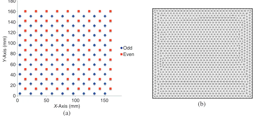
Figure 3. (a) Odd-Even sampling pattern over phantom; (b) 16.5×16.5 cm FE mesh — extruded to 3.0 cm thickness.

6.0 mm above the slab. The first sampling horizon keeps the coil parallel to the slab and spaced 2.0 mm above the slab. All other sampling horizons allowed for random coil tilt, with axis tilted as much as 5 degrees from vertical, which alters the height of coil center. Allowing for coil tilt when the coil is clear of the slab better mimics an actual hand scan where coil tilt is unavoidable.

The phantoms shown in Figure 2 provide an effective test of the algorithm’s ability to resolve structure over its 3.0 cm depth. Resolving lateral, or XY structure should be less difficult since both strip separation and width are∼1 coil diameter. However, as Figure 1(b) suggests, resolving a correct conductivity profile to a depth of 3.0 cm appears more challenging since sampling level at a depth of 1.5 cm has already fallen to 5% of the maximum found at the target boundary, with coil ‘R’.

Since all real measurements are contaminated by noise, Gaussian-distributed noise is added to virtual coil loss measurements over each phantom. A base level of noise is added to all “pristine” data to match the noise level of current instrumentation. However, in one additional experiment, Gaussian noise is increased 5×to correspond to older instrumentation. Experimental coil loss is obtained through measurement of the real part of coil admittanceY_re while in the vicinity of coil resonance. Admittance change relative to a free space admittance measurement is used to get coil loss [8]:

R_loss=ω2L2δY_re (20)

Older instrumentation measured admittance with a precision of±0.12µS, while newer instrumentation measures admittance with a precision of ±0.025µS. Further processing of experimental data with Savitzky-Golay denoising yields a precision level of ±0.01µS in current instrumentation, which corresponds to a loss precision of ±0.000286 ohms — using a frequency of 12.5 MHz and inductance equal to 2.155µH. This amount of loss uncertainty is used to compute a Gaussian noise component that is added to each of the 486 computed virtual loss values. The coil loss uncertainty can also be used to provide an error bound, and stopping condition as previously discussed, for Equation (13) or (14). Since there are 486 coil loss “measurements”, the loss uncertainty for a single solution component is multiplied by √486, giving an error norm for Equation (14) of 0.0063 ohms. In one instance, noise is increased 5×to assess its effect on image reconstruction.

6. IMAGE RECONSTRUCTION RESULTS

(a)

(b) _(c)

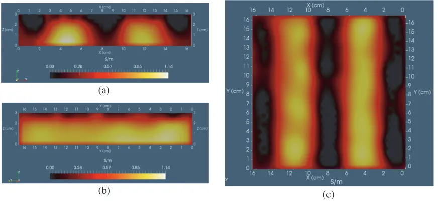
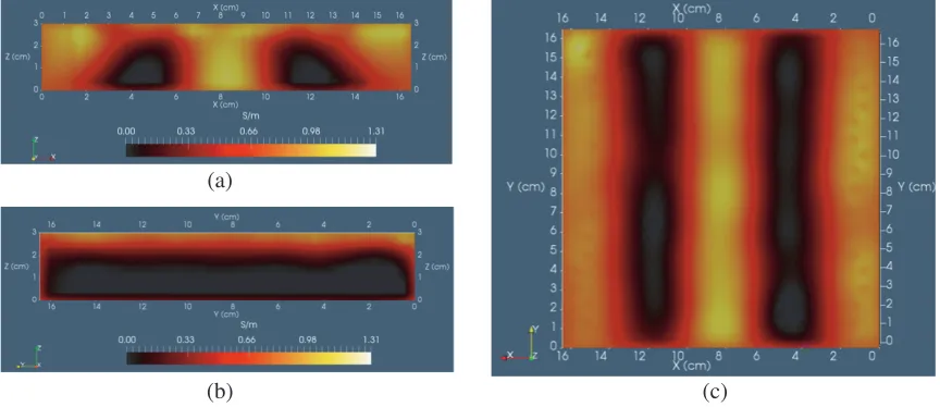
Figure 4. Image reconstructions for phantom having buried high conductivity (1 S/m) strips in a low conductivity (∼0 S/m) background; slice (a) normal toY-axis; slice (b) normal to X-axis,X∼4.5 cm; slice (c) normal toZ-axis;β0 ≈0.267 S/m from (12) to set shift.

singular values, which decrease monotonically from a maximum value at j = 1 to a smallest value at

j = 486 (number of measurements, in this case). For the phantom consisting of two buried strips of 1.0 S/m material, j = 220 was selected, which gave an error norm of 0.0047 ohms, close to the target of 0.0063 ohms. The non-dimensional decay parameter discussed in Equation (19) was set to 1.0, as suggested by exponential fits to the ‘R’ curve in Figure 1(b). Convergence is obtained after 6 iterations of the active set method. Three image slices are shown in Figure 4 — a transverse slice midway along and normal to the Y-axis, a longitudinal slice normal to the X-axis at X ∼ 4.5 cm, and finally, a

Z-normal slice at Z ∼ 1.5 cm (midway along the Z-axis). To facilitate comparison, these same slice locations are used in all images that follow.

Each slice in Figure 4 indicates that image reconstruction from 486 measurements does a reasonably good job of faithfully representing the original phantom in Figure 2. Conductivity spans from 0.0 to

∼1.0 S/m, as it should; conductivity stays near 0.0 S/m in the space separating the two strips, from the top of the phantom all the way to the bottom; and, features are arranged in spatially correct position. Of particular importance, variation of structural features with respect to depth track rather well those of the actual phantom, suggesting that the diagonal regularization matrix is performing as intended.

As stated, setting the decay parameter in Equation (19) to 1.0 was based upon Figure 1(b) data. Of interest is the effect of setting it to zero (equal weighting), which is shown in a single slice, normal to the Y-axis (transverse to strips) in Figure 5. The image in Figure 5 is also based upon setting τ

equal to singular valuej= 220, with resulting error norm = 0.0059 ohms (near the stopping condition). Comparing the transverse slices of Figures 4 and 5, we note that when solution components are equally weighted in the penalty term (η ≈ 0, Equation (19)), conductivity in between or to either side of the strips struggles more so to stay near zero over the complete depth of the field compared with the case when decay parameter is set to 1.0. The effect is perhaps more noticeable inside the strips, where in Figure 5, conductivity is considerably higher near the upper portions of the strips. If the decay parameter is increased to η ≈ 1.5, conductivity inside the strips is skewed more toward the bottom, suggesting that 1.0 was near optimal.

Figure 5. Slice transverse to 1.0 S/m strips, corresponding to transverse image in Figure 4 — except that now, the decay parameter = 0, impairing depth resolution; note that conductivity is skewed upward too much inside strips compared to the corresponding slice in Figure 4 that sets η= 1.

(a)

(b) (c)

Figure 6. Image reconstructions for phantom having buried low conductivity (∼ 0 S/m) strips in a high conductivity (1.0 S/m) background; slice (a) normal toY-axis; slice (b) normal to X-axis; slice (c) normal toZ-axis;β0 ≈0.73 S/m from (12) to set shift.

error norm value as well. Figure 6 shows slice locations that correspond to those of Figure 4, but with an expected image inversion of the electrical conductivity distribution. Remarkably, the longitudinal slice along the length of the low-conductivity strip cleanly reveals the thin layer of high conductivity material just above the strip’s entire length.

The reconstructed images shown in Figure 6 for buried low conductivity strips again do a reasonable job of faithfully matching the features of the actual phantom shown in Figure 2. Though not apparent in the slices of Figure 6, very few locations inside the full 3D image exhibit conductivity near the maximum of ∼ 1.31 S/m shown on the side scale — just a spot near a corner of the upper boundary where sampling is least adequate. Thus, most regions outside the strips are near the 1.0 S/m maximum conductivity, as expected. Perhaps most satisfying is the ability to depth-resolve the slab, especially the electrical conductivity distribution inside the strips and in the space between them. Depth-resolving the regions of the slab nearer the sides is more problematic since the scan includes fewer coil loss values there.

(a)

(b) (c)

Figure 7. 5× higher noise version of Figure 6. Phantom has buried low conductivity (∼0 S/m) strips in a high conductivity (1.0 S/m) background; slice (a) normal to Y-axis; slice (b) normal to X-axis; slice (c) normal toZ-axis;β0 ≈0.73 S/m from (12) to set shift.

compared to those in Figure 6 — color transition levels for red and yellow are set to match those in Figure 6 to aid direct comparison (though the difference is barely noticeable).

As expected, this algorithm is not immune to noise — note that geometrical distortions start to develop, which are perhaps most noticeable in the Z-normal slice (image (c)) where strips become wavy. Nevertheless, features continue to be correctly located and readily identifiable relative to the true objects shown in Figure 2. There may be a tendency to want more smoothing. However, we believe it is best to allow the effects of noise to appear in an MIT image reconstruction since even though additional smoothing will help to suppress noise, further smoothing will also remove genuine features or structure from the MIT image.

Finally, we briefly consider a different weighting scheme than the exponential weights proposed in Equation (19). As suggested in Section 4, “Setting Weights”, we could directly use the sampling curves plotted in Figure 1(b) — though theZ coordinate needs to be scaled since using the plotted curves “as is” would tend to overemphasize deeper locations. Weights are based on the kernel function given in Equation (18):

d_j =G(ρ, z_scale) ; z_scale =ηz_j/zmax, (21)

The scaling parameters have the same significance as before — we just have a different function than exponential. An important difference is that we have to choose a distance from the coil axis for creating weights. Here, the chosen distance is simply the location where G would be maximum along the radial direction — see the plot in Figure 1(a), ∼ 1.5 cm (coil ‘R’). Image reconstruction based upon Equation (21) sets the decay parameter η∼0.3, and with stopping conditions as previously described, singular values having index equal to 220 and 210 were used for buried 1.0 S/m and 0.0 S/m strips respectively.

Clearly, the images shown in Figures 8(a)–(b) do not appear much different than the corresponding images given in Figures 4(a) and 6(a). There is a greater tendency for the “kernel-weighted” images to better preserve the square cross sections of the strips — though the exponential weighting parameters could possibly be tweaked to achieve a cross section similar to those in Figures 8(a)–(b).

(a)

(b)

(c)

Figure 8. (a)–(b) Weights based upon the kernel function given in (18), though scaling as prescribed by (21) — these slices may be compared with the alternative exponential scaling illustrated by the transverse slices shown in Figures 4 and 6 ((a) images); (c) image reconstruction corresponding to (a), but using the method previously reported by Feldkamp [8].

7. DISCUSSION AND CONCLUSIONS

The regularization or penalty term used here departs from what was used previously in this particular application of single-coil MIT. Before, the regularization matrix consisted of the three components of the conductivity gradient, computed for each element, so that rapidly varying solutions became more heavily penalized as τ increased. Also, an L-curve approach was used to determine a suitable value for the regularization parameter, which worked well but contributed to increased computational overhead. Compared to the images produced by this newer algorithm, the prior approach caused too much smoothing, so that geometrical feature accuracy tended to be less — as noted in Figure 8(c). Furthermore, there were localization issues that could not be corrected, as they are here by appropriate use of the penalty shift and penalty weights applied individually to solution components. Also, the prior formulation was not put into “standard form”, as we have done here. As a result, the newer algorithm is much more efficient, running∼50×faster than our older algorithm — even though the new method is run on a single core while the old method ran on 12 cores.

which very quickly provides a solution and opportunity to check status, and then gradually progresses to the stopping condition. As the stopping condition is approached, the time to acquire a solution becomes longer, as expected due to increasing size of the active set — which is itself a consequence of reduced filtering. The image reconstructions performed in this work took∼7 minutes on a single core of a Mac Book Pro (2013 build). Nearly half of that time was used to compute the model matrix ˜A.

In our application, the diagonal regularization matrix imposed a higher penalty at those points nearest the boundary of the target, where proximity to the coil was highly likely during the course of a scan. Such an approach is necessary since otherwise, near-boundary nodes would have an outsized advantage during image reconstruction — a direct result of their greater immunity to coil loss measurement noise compared with nodes located at greater depth within a target. The situation is not unlike that encountered in CT X-ray where particular pathways through a medium lead to much greater beam attenuation than others, so that in the absence of compensation, artifacts can develop. Indeed, a diagonal “weighting” matrix has been proposed for CT image reconstruction, resembling what is used here, that applies weights to the residual error norm in accordance with the intensity of signal that exits the target [24]. Our weighting strategy works well provided that points very distant from any one of the locations where the coil visits aren’t permitted to exhibit unusually high conductivity values. Though not encountered here, this potential problem could be managed by creating a space or region outside of some “preferred zone” that encompasses the space we really care about, and specifically setting a very high penalty for those outer locations. That would have the desired effect of forcing the solution outside of the “preferred zone” to remain close to some known average conductivity and therefore contribute little if anything to the predicted measurement.

This new algorithm has already been put to work on laboratory phantoms, either biological in origin or derived from agarose and fat. In a recent example reported by Feldkamp and Quirk [25], a cross-cut veal shank was scanned with modified older instrumentation and configured so that IR optical tracking could seamlessly provide coil position and orientation data [26] while acquiring inductive loss. Image reconstruction with the algorithm reported here was shown to faithfully reveal the structure of the veal shank — bone, fat seams and muscle partitions.

As already noted, efficiency is greatly improved in this algorithm compared to its predecessor, though is highly dependent upon maintaining a relatively small active set. Though not an issue as of yet, very large active sets could potentially arise in specimens comprised primarily of fat, which has a conductivity near zero. In such cases, it may be that use of an L1 penalty term could provide a superior path for inversion of the convolution integral considered here. Indeed, the work of Fang et al. [27] provides encouraging results in an MIT setting, suggesting that inversion of the convolution integral might indeed be better accomplished byL1 regularization.

REFERENCES

1. Gabriel, C., S. Gabriel, and E. Courthout, “The dielectric properties of biological tissues: I. Literature survey,”Phys. Med. Biol., Vol. 41, 2231–2249, 1996.

2. Joines, M. T., Y. Zhang, C. Li, and R. L. Jirtle, “The measured electrical properties of normal and malignant human tissues from 50 to 900 MHz,”Medical Physics, Vol. 21, No. 4, 547–550, 1994. 3. Haemmerich, D., S. T. Staelin, J. Z. Tsai, S. Tungjitkusolmun, D. M. Mahvi, and J. G. Webster,

“In vivo electrical conductivity of hepatic tumors,”Physiol. Meas., Vol. 24, 251–260, 2003.

4. Kim, H., A. Merrow, S. Shiraj, B. Wong, P. Horn, and T. Laor, “Analysis of fatty infiltration and inflammation of the pelvic and thigh muscles in boys with Duchenne muscular dystrophy: Grading of the disease involvement on MR imaging and correlation with clinical assessments,” Pediatric Radiology, Vol. 43, No. 10, 1327–1335, 2013.

5. Borcea, L., “Electrical impedance tomography, Inverse Problems, Vol. 18, R99–R136, 2002. 6. Wei, H. Y. and M. Soleimani, “Electromagnetic tomography for medical and industrial applications:

challenges and opportunities,”Proc. IEEE, Vol. 101, 559–564, 2013.

8. Feldkamp, J. R., “Single-coil magnetic induction tomographic three-dimensional imaging,” J. Medical Imaging, Vol. 2, No. 1, 013502, 2015.

9. Feldkamp, J. R. and S. Quirk, “Effects of tissue heterogeneity on single-coil, scanning MIT imaging,”Proc. SPIE 9783, Medical Imaging 2016: Physics of Medical Imaging, 978359, March 25, 2016.

10. Zaman, A. J. M., S. A. Long, and C. G. Gardner, “The impedance of a single-turn coil near a conducting half space,”J. Nondestructive Eval., Vol. 1, No. 3, 183–189, 1980.

11. Feldkamp, J. R. and S. Quirk, “Validation of a convolution integral for conductivity imaging,”

Progress In Electromagnetic Research Letters, Vol. 67, 1–6, 2017.

12. Katamreddy, S. H. and P. K. Yalavarthy, “Model-resolution based regularization improves near infrared diffuse optical tomography,” J. Opt. Soc. Am., Vol. 29, No. 5, 649–656, 2012.

13. Haskell, K. H. and R. J. Hanson, “An algorithm for linear least squares problems with equality and nonnegativity constraints,”Math. Program, Vol. 21, 98–118, 1981.

14. Bj¨orck, ¨A., “Numerical methods for least squares problems,” Society for Industrial and Applied Mathematics, Philadelphia, 1996.

15. Mead, J. L. and R. A. Renaut, “Least squares problems with inequality constraints as quadratic constraints,” Linear Algebra and Its Applications, Vol. 432, 1936–1949, 2010.

16. Hansen, P. C., “Relations between SVD and GSVD of discrete regularization problems in standard and general form,” Linear Algebra and Its Applications, Vol. 141, 165–176, 1990.

17. Donatelli, M., A. Neuman, and L. Reichel, “Square regularization matrices for large linear discrete ill-posed problems,” Numerical Linear Algebra with Applications, Vol. 19, 896–913, 2012.

18. Eld´en, L., “Algorithms for the regularization of ill-conditioned least squares problems,” BIT, Vol. 17, 134–145, 1977.

19. Chen, D. and R. J. Plemmons, “Nonnegativity constraints in numerical analysis,”Proceedings: The Birth of Numerical Analysis, 109–140, Leuven Belgium, 2009.

20. Engl, H. W., “On the choice of the regularization parameter for iterated Tikhonov regularization of ill-posed problems,”J. of Approximation Theory, Vol. 49, 55–63, 1987.

21. Hochstenbach, M. and L. Reichel, “An iterative method for Tikhonov regularization with a general linear regularization operator,” J. Integral Equ. Appl., Vol. 22, 463–480, 2010.

22. Gradshteyn I. S. and Ryzhik, Table of Integrals, Series and Products, Corrected and Enlarged Edition, A. Jeffrey, Academic Press, New York, NY, 1980.

23. Lapidus, L. and G. F. Pinder,Numerical Solution of Partial Differential Equations in Science and Engineering, Wiley-Interscience, J. Wiley & Sons, NY, 1982.

24. Thibault, J.-B., K. D. Sauer, C. A. Bouman, and J. Hsieh, “A three-dimensional statistical approach to improved image quality for multislice helical CT,”Medical Physics, Vol. 4, No. 11, 4526–4544, 2007.

25. Feldkamp, J. R. and S. Quirk, “Optically tracked, single-coil, scanning magnetic induction tomography,” Proc. SPIE 10132, Medical Imaging 2017: Physics of Medical Imaging, 10132P, March 9, 2017.

26. Wiles, A. D., D. G. Thompson, and D. D. Frantz, “Accuracy assessment and interpretation for optical tracking systems,”Medical Imaging Proceedings (SPIE) 5367; Visualization, Image-Guided Procedures, and Display, 433, 2004.