Optimization of LPDA Excitations and the PBM Antenna Benchmarks Using SHADE and L-SHADE Algorithms

Optimization of LPDA Excitations and the PBM Antenna

Benchmarks Using SHADE and L-SHADE Algorithms

Richard A. Formato1, * and Mahamed G. H. Omran2

Abstract—The SHADE and L-SHADE variants of the Differential Evolution global search and optimization algorithm are used to compute optimized excitations for a Log Periodic Dipole Array antenna and to numerically solve the Pantoja-Bretones-Martin suite of antenna benchmark problems. Comparison to published data shows that SHADE and L-SHADE both are effective and efficient algorithms for solving the array excitation problem and the Pantoja-Bretones-Martin wire antenna benchmarks. L-SHADE clearly is more efficient on the array problem, but overall on the benchmarks the opposite is true, albeit to a lesser degree. The data support the view that neither algorithm is generally better than the other for the type of wire antenna problems considered here. Rather, which algorithm is more efficient is highly dependent on the specific antenna being optimized. In terms of the quality of their solutions, however, both algorithms accurately return the benchmarks’ known global optima while both converge on different optimal array excitations that result in very similar objective function fitnesses.

1. INTRODUCTION

Global search and optimization algorithms (GSO) have become an important tool in antenna design and optimization (DO). A plethora of algorithms has been applied to a wide range of problems, for example: invasive weed optimization of a PCB UWB antenna [1]; genetic algorithm (GA), particle swarm (PSO) and differential evolution (DE) optimization of circular arrays [2]; GA design of a mobile base station antenna [3]; binary DE antenna design [4]; sparse array design using self-adaptive DE [5]; planar array synthesis using modified PSO [6]; DE/PSO/GA optimization of microstrip antennas [7]; sidelobe and null level optimization with ant colony optimization (ACO) [8]; wideband antenna design using hybrid DE and ACO [9]; and linear array synthesis using DE with convex programming [10]. While these examples emphasize DE because the SHADE algorithms are DE variants, there are many other algorithms applied to antenna DO (see, for example, [11–19]). These are but a few representative examples drawn from hundreds, perhaps thousands, of GSO-based antenna DO problems.

This paper introduces the mix of two new algorithms: SHADE and L-SHADE, both variants of Differential Evolution. They are tested against several antenna optimization problems: (i) determining excitations in a Log Periodic Dipole Array (LPDA) antenna, and (ii) solving the five antenna problems comprising the Pantoja-Bretones-Martin (PBM) benchmark suite [20]. Section 2 of this paper describes SHADE and L-SHADE. Section 3 discusses the LPDA problem and Section 4 the PBM problems. The data show that SHADE and L-SHADE are very effective and efficient optimizers for the type of antenna DO considered here. Section 5 is the Conclusion. The Appendix describes the PBM benchmarks in detail.

Received 7 October 2017, Accepted 17 November 2017, Scheduled 4 December 2017 * Corresponding author: Richard A. Formato ([email protected]).

1 _{Consulting Engineer & Reg. Patent Attorney, Of Counsel Emeritus, Cataldo & Fisher, LLC, P. O. Box 1714, Harwich, MA 02645,}

2. SHADE AND L-SHADE ALGORITHMS

Differential Evolution (DE) was proposed by Storn and Price [21] to find the global optimum of nonlinear, non-convex, multimodal, and non-differentiable functions defined in a continuous search space. DE and its variants stand out as very competitive optimizers that have been successfully used to solve many real-world engineering problems [22]. DE is known for its simple structure, ease of use, robustness, and speed [23]. Many attempts have been made to improve DE’s performance, two recent and efficient ones being Success-History based parameter Adaptation DE (SHADE) [24] and its improved variant L-SHADE [25]. SHADE ranked third out of twenty one algorithms in the 2013 IEEE CEC competition on real parameter single-objective optimization (the first two ranked algorithms were non-DE) [26]. In the 2014 IEEE CECE competition on real parameter single-objective optimization L-SHADE yielded the best performance among all non-hybrid algorithms [27].

2.1. Canonical Differential Evolution

A DE population is a set of real-parameter vectors x_i =x1, . . . , xD where i∈ {1,2, . . . N}, and Dis the problem’s dimensionality.

First, a population of potential solutions is randomly generated within the search or decision space (DS) constrained by its lower and upper bounds,aand b, respectively, using the following formula:

x_i,j(0) =a_j+r(b_j−a_j) (1)

where r is a uniformly-distributed random number generated from the interval [0,1], i∈ {1,2, . . . , N}, and j∈ {1,2, . . . D}.

After initializing its population, the DE algorithm comprises three steps that are repeated until a stopping criterion is satisfied: (i) Mutation; (ii) Crossover; and (iii) Selection. The DE algorithm is briefly shown as Alg. 1 in Fig. 1, and its three steps are explained below.

Alg. 1: The canonical DE algorithm.

initialization

while a stopping criterion is not satisfied do for each vector in the population do

mutation crossover selection

endfor endwhile

Figure 1. Differential evolution pseudocode.

2.1.1. Mutation

A mutant vector, v_i, is created for each population member,u_i, in the current iteration as follows.

v_i(t) = x_r1(t) +F(xr2(t)−xr3(t)) (2)

where r1, r2, and r3 are randomly chosen from [1, N] such that they differ from each other as well as

from i. The scaling factor, F, is a positive parameter (F ∈ (0,1]) that controls the magnitude of the difference vector. Eq. (2) describesDE/rand/1, which is the most commonly used mutation strategy. Another mutation strategy, DE/current-to-best/1, employs the following equation to generate a mutant vector:

vi(t) = xi(t) +F(xbest(t)−xi(t)) +F(xr1(t)−xr2(t)) (3)

2.1.2. Crossover

A trial vector,u_i(t), is generated by mixing the components of the target vector,x_i(t), and the mutant vector, v_i(t), as follows.

ui,j(t) =

v_i,j if j=J orr≤Cr

x_i,j otherwise (4)

where Cr is the pre-fixed crossover rate; r is a uniformly distributed random number in [0,1); and J is a randomly chosen number in the set {1,2, . . . , D}, thereby insuring that u_i(t) inherits at least one component from v_i(t). This process is called Binomial Crossover and is the most commonly used DE crossover operator.

2.1.3. Selection

After generating the set of the trial vectors, a greedy selection process is used to determine survivors for the next iteration as follows:

x_i(t+ 1) =

u_i(t) if f(u_i(t))≤f(x_i(t)) xi(t) otherwise

(5)

where f(•) is the objective function to be optimized (minimized or maximized depending on the problem). The equality in “≤” of Eq. (5) helps DE to navigate “flat” fitness landscapes by reducing the possibility of stagnation [22].

2.2. SHADE

The parametersF andCrhave a profound effect on DE’s performance. Tanabe and Fukunaga therefore proposed the SHADE algorithm [24] to take advantage of their success history in exploring DS. SHADE maintains memory archives MCr and MF, respectively, which store a total of H values of Cr and F that have performed well in recent previous iterations.

At each iteration, t, there are two control parameters Fi and CRi for each vector xi. They are initially set to 0.5, and they are updated by randomly choosing an index ri in [1, H] and applying the following update equations:

F_i ∼ Cauchy(M_F,ri,0.1) (6)

Cr_i =

0 ifMCr,ri =⊥

N(M_Cr,ri,0.1) otherwise (7)

where Cauchy (M_F,ri,0.1) is a Cauchy-distributed random variable with location parameterM_F,ri and scale parameter 0.1; N(M_Cr,ri,0.1) is a Gaussian distribution with mean M_Cr,ri, standard deviation 0.1; and⊥is theterminal value. IfF_i>1, thenF_i = 1. IfF_i ≤0, then Eq. (6) is repeated until a valid value is generated. Once F_i is determined, then Cr_i is updated according to Eq. (7). If the new value of Cri ∈/[0,1], then it is replaced by the boundary value, that is 0 or 1, closest to the generated value. AfterFi andCri have been updated for each vector xi, a mutant vector, vi(t), is generated using thecurrent-to-pbest/1mutation strategy [28], which is a variant of thecurrent-to-best/1strategy discussed in the previous section. Thegreediness of current-to-pbest/1is adjusted using a parameter p∈(0,1] as follows:

v_i(t) = x_i(t) +F_i(x_pbest(t)−x_i(t)) +F_i(x_r1(t)−xr2(t)) (8)

where x_pbest(t) is randomly chosen from the top N ×p individuals in iteration t. Parameter p balances exploration and exploitation, with smaller values favoring exploitation while larger ones favor exploration.

SHADE maintains diversity in its population by utilizing anexternal archive that contains parent vectors x_i(t) that are worse than the trial vectors u_i(t). In Eq. (8), x_r2(t) is selected from the union

If a boundary-constraint violation occurs, then it is corrected as follows:

v_i,j(t) =

⎧ ⎪ ⎨ ⎪ ⎩

(aj+xi,j(t))

2 if vi,j(t)< aj (b_j+x_i,j(t))

2 if vi,j(t)> bj

(9)

After generating the mutant vectorvi(t), the binomial crossover of Eq. (4) is used to generate the trial vector u_i(t). After generating all trial vectors, the greedy selection of Eq. (5) is used to create a new population. Values creating a trial vector u_i(t) that is better than the target vector x_i(t) are recoded as S_Cr and S_F.

This process is repeated iteration-by-iteration, and at the end of each iteration the historical memory contents are updated using Alg. 2 in Fig. 2. At each iteration, the kth (1≤k≤H) entries in the two historical memory archives are also updated. Initially set to k = 1, this index is incremented when a new element is inserted into the archive. If k > H, k is reset to 1. Note that the memory archives are not updated when all vectors at iteration t fail to generate better trial vectors, that is, SCr=SF =∅.

Alg. 2. Historical memory update algorithm in SHADE.

ifSCr and then

ifM == Cr,k,t or max(SCr) == 0 then MCr,k,t+1=

else

MCr,k,t+1 meanWL endif

MF,k,t+1 meanWL k + +

ifk > H then k =1

endif else

MCr,k,t+1

MF,k,t+1

endif

=/ SF =/

⊥ ⊥

⊥

= (S Cr)

= (S F)

= MCr,k,t = M_F,k,t

Figure 2. DE pseudocode with history data.

Mean values are computed as follows using a weighted Lehmer mean, denoted mean_{W L}(S), which has the effect of favoring larger values:

mean_{W L}(S) = |S|

k=1

w_kS_k2

|S|

k=1

w_kS_k

, (10)

wherew_k = Δfk |S|

l=1

Δf_l

, Δf_k =|f(u_k(t))−f(x_k(t))|.

2.3. L-SHADE

Tanabe and Fukunaga further improved SHADE by linearly reducing its population size during the course of a run [25]. The new algorithm, called L-SHADE, starts with an initial population size ofN_init vectors that is reduced iteration-by-iteration as follows:

N(t+ 1) = round

N_init−Nmin

max nf e nf e+Ninit (11)

where t is the iteration number, Nmin the smallest possible value for the population size, nf e the

current number of objective function evaluations, and max nf e the maximum number of objective function evaluations. In L-SHADE, Nmin = 4 because the current-to-pbest mutation operator,

Eq. (8), requires four vectors. Whenever N(t+ 1) < N(t), only the best N(t)−N(t+ 1) vectors survive to the next iteration, and the archive size is readjusted according to the then current population size. Numerical experiments have shown that L-SHADE generally outperforms SHADE [25].

2.4. Experimental Setup

The following setup parameters were used for all optimization runs reported here: For SHADE,N was set to 100, and other parameters were set as suggested in the SHADE code posted online by R. Tanabe†, viz, p = 0.11; H = D; archive size = 2N. For L-SHADE, the values of the control parameters were also the same as those in the online source code†, viz, N_init = 18D; p = 0.11; H = 5; archive size = 1.4N. Twenty five independent runs were made for each antenna problem, and a run was terminated when either of the following criteria was met: (i) no improvement in best solution for 20 consecutive iterations; or (ii) maximum number of function evaluations max nf e was reached.

3. LPDA EXCITATION OPTIMIZATION

The objective of the LPDA problem is to determine a set of excitations that produces an omnidirectional H-plane radiation pattern at a set of predefined frequencies. The Log Periodic Dipole Array antenna, introduced by Isbell in 1960 [29], has gained widespread acceptance as a moderate gain broadband structure [30, 31]. Each dipole in the array bears a fixed geometrical relationship to its neighbors that is determined by a single scaling parameter τ as follows:

1 τ =

L_n+1

Ln

= Dn+1 Dn

= gn+1 gn

= Sn+1 Sn

whereLn,Dn,gn, and Sn, respectively, are thenth dipole’s overall length, element diameter, feed gap length, and spacing from the (n−1)st dipole [31 @ Ch. 11].

With ultra-wideband applications in mind, for example radio astronomy, communications systems, and radar, Yang published in 2010 a theoretical development of the conditions necessary for obtaining constant radiation characteristics from log-periodic arrays [32]. The planar 5-dipole LPDA described in that paper forms the basis for subsequent work on the excitation problem by Lehmensiek and de Villiers [33, 34]. Only numerical optimization can accurately solve the excitation problem because the analytical approach incorrectly assumes only fundamental current modes on each dipole. Consequently, Brute Force optimization was used in [33] and Population-Based Incremental Learning/Nelder–Mead Simplex in [34].

SHADE and L-SHADE are applied to the LPDA problem using the parameters in Section 2.4. The fitness (objective) function, to be minimized, is the deviation from a perfectly uniform (circular) H -plane far field radiation pattern, that is, Min [Gmax(∅= 0)−Gmin(∅= 0)] where theG’s are maximum

and minimum H-plane gains, respectively. The array was modeled with Version 2 of the Numerical Electromagnetics Code [35]. NEC2 is a widely used Method of Moments (MoM) code for modeling wire antennas (in [34] a commercial MoM code was used). For convenience, frequencies and dimensions were scaled to 299.8 MHz (λ = 1 m). PEC (Perfect Electric Conductor) dipoles are assumed so that conductivity was not scaled.

Table 1. 5-Dipole LPDA geometry.

L_n (mm) R_n(mm) X0,n (mm) 68.63τn−1 0.776τn−1 40.92τn−1

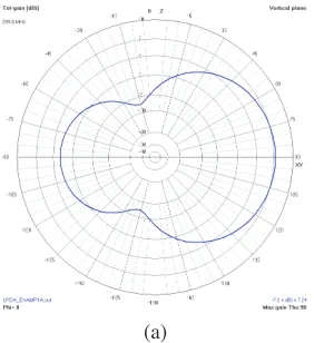
The LPDA geometry is summarized in Table 1 whereinn= 1, . . . ,5 andτ = _1.1₁₈ (same value used in [34]). Ln,RnandX0,n, respectively, are the dipole end-to-end length, wire radius, and distance along the +X-axis (NEC employs standard right-handed Cartesian [x, y, z] and spherical [ρ, θ, ϕ] coordinates). A perspective view of the antenna appears in Fig. 3 (axis length 0.2 m, dipole #1 being the longest). Optimization was performed in the 2.576–4.995 GHz band at the same five logarithmically spaced frequencies used in [34], that is, f1 = f2·τ; f2 = 3.04 GHz; f3 = f2/τ; f4 = f2/τ2; and f5 = f2/τ3

(scaled as described above).

Figure 3. LPDA perspective view.

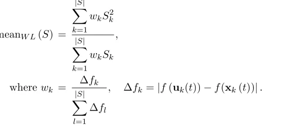
The H-plane radiation pattern with only the first dipole excited is shown in Fig. 4. It is highly distorted as expected due to the fields scattered by the other dipoles. When all five dipoles are driven with optimized excitations, however, the resulting pattern is shown in Fig. 5. It is very nearly omnidirectional as required, that is, essentially the pattern of a single dipole without the others being present. Controlling theH-plane pattern is accomplished by using SHADE and L-SHADE to compute an optimized set of excitations that, in effect, render electromagnetically “invisible” all but one of the dipoles.

(a) (b)

(a) (b)

Figure 5. H-plane radiation pattern, 5 dipoles driven, optimized excitation.

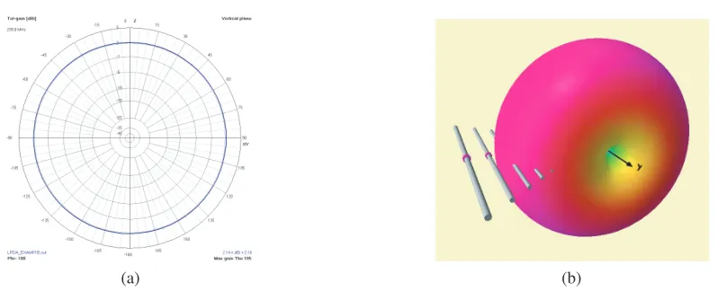
Table 2. SHADE optimized 5-frequency LPDA excitations.

Excitation f1 = 2.576 GHz

f2 =

3.040 GHz

f3 =

3.587 GHz

f4 =

4.233 GHz

f5 =

4.995 GHz

V1 _∠1v_{0◦ ∠301}1.464v_{.863◦ ∠286}1.212v_{.637◦ ∠316}0.380v_{.604◦ ∠}1.691v_41.400◦

V2 _∠0.852v_29.698◦ _∠1v₀◦ _∠3451.616v_.053◦ _∠3302.403v_.953◦ _∠2.411v_91.613◦

V3 _∠0.607v_{27.823◦ ∠330}1.775v_{.345◦ ∠}1v_{0◦ ∠295}2.193v_{.770◦ ∠}2.624v_58.742◦

V4 _∠3350.815v_{.746◦ ∠302}1.773v_{.798◦ ∠326}0.701v_{.215◦ ∠}1v_{0◦ ∠}1.326v_31.461◦

V5 _∠2290.281_.808◦ _∠2762.545v_.356◦ _∠2980.066v_.975◦ _∠3030.559v_.709◦ _∠1v₀◦

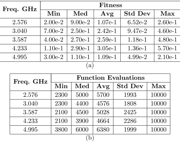
Tables 2 and 3, respectively, contain the SHADE- and L-SHADE-computed optimized excitations. Following the protocol used in [34] a reference excitation of 1 volt∠0◦is applied to thenth dipole at each frequencyf_n,n= 1, . . . , 5. SHADE returned best fitnesses (maximum deviations from omnidirectional) of 0.02, 0.07, 0.04, 0.01 and 0.03 dB, respectively, at frequenciesf1,f2,f3,f4, and f5. Because NEC2’s

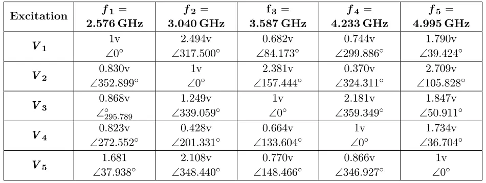
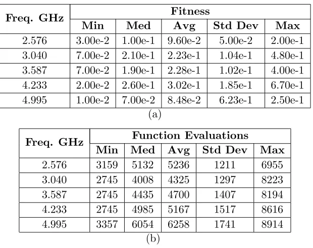
gain resolution is 0.01 dB, only a value of zero would be better. The corresponding 5-frequency L-SHADE best fitnesses are 0.03, 0.07, 0.07, 0.02 and 0.01 dB. Both L-SHADE variants achieve quite similar levels of H-plane pattern uniformity, neither algorithm being clearly superior to the other, and both returned quite good results from an engineering application point of view. Note that, like [34], this study is limited to determining the required excitations, not implementing them.

Lehmensiek and de Villiers conclude in [34] that there is no unique, well-defined set of excitations that achieves omnidirectionality, their conclusion resting on interpreting the voltage-phase scatter plots in [34]. This hypothesis is supported by the SHADE/L-SHADE data. The optimized excitations in Tables 2 and 3 are quite different, yet they achieve quite similar levels of pattern uniformity, which is convincing evidence that, as suggested in [34], there is no single global optimum. An omnidirectional pattern may be achieved by widely different excitations, and different optimizers will likely return different results that accomplish the same objective.

Table 3. L-SHADE optimized 5-frequency LPDA excitations.

Excitation f1 = 2.576 GHz

f2 = 3.040 GHz

f₃ = 3.587 GHz

f4 = 4.233 GHz

f5 = 4.995 GHz

V1 _∠1v₀◦

2.494v

∠317.500◦

0.682v

∠84.173◦

0.744v

∠299.886◦

1.790v

∠39.424◦

V2 _∠3520.830v_{.899◦ ∠}1v_{0◦ ∠157}2.381v_{.444◦ ∠324}0.370v_{.311◦ ∠105}2.709v_.828◦

V3 _∠0.868v◦

295.789

1.249v

∠339.059◦

1v

∠0◦

2.181v

∠359.349◦

1.847v

∠50.911◦

V4 _∠2720.823v_{.552◦ ∠201}0.428v_{.331◦ ∠133}0.664v_{.604◦ ∠}1v_{0◦ ∠}1.734v_36.704◦

V5 _∠371.681_{.938◦ ∠348}2.108v_{.440◦ ∠148}0.770v_{.466◦ ∠346}0.866v_{.927◦ ∠}1v_0◦

Table 4. SHADE optimized 8-frequency LPDA excitations∗.

Frequency

(GHz) V1 V2 V4 V5

3.14232 1.889v

∠310.049◦

1.781v

∠353.530◦

0.468v

∠321.360◦

0.467v

∠381.075◦

3.24808 1.258v

∠348.395◦

1.752v

∠1.535◦

0.770v

∠301.666◦

2.045v

∠380.175◦

3.35740 0.816v

∠212.072◦

2.484v

∠209.305◦

0.093v

∠281.402◦

2.903v

∠230.544◦

3.47040 1.334v

∠37.110◦

2.307v

∠73.257◦

1.1018v

∠63.801◦

1.700v

∠146.014◦

3.7093 0.500v

∠310.663◦

0.818v

∠327.858◦

0.400v

∠398.905◦

0.034v

∠152.153◦

3.83273 1.356v∠271.604◦ 2.610v ∠334.773◦ 0.378v∠361.103◦ 0.130v

∠287.817◦

3.96173 2.128v

∠78.369◦

2.742v

∠45.671◦

0.059v

∠150.336◦

0.269v

∠334.196◦

4.09507 1.270v

∠288.363◦

2.256v

∠306.833◦

2.250v

∠6.315◦

1.130v

∠324.904◦ ∗_{V3 =1v∠0}◦

Table 5. L-SHADE optimized 8-frequency LPDA excitations∗.

Frequency (GHz) V₁ V₂ V₄ V₅

3.14232 2.255v

∠336.261◦

1.934v

∠397.182◦

0.204v

∠307.550◦

1.337v

∠341.448◦

3.24808 1.287v

∠308.724◦

2.042v

∠309.620◦

0.758v

∠300.926◦

1.182v

∠357.915◦

3.35740 1.010v

∠361.220◦

2.283v

∠15.796◦

1.261v

∠376.759◦

0.776v

∠18.441◦

3.47040 2.004v

∠370.422◦

2.680v

∠382.074◦

1.340v

∠364.680◦

2.352v

∠48.624◦

3.7093 1.169v

∠312.013◦

2.852v

∠348.803◦

1.286v

∠387.863◦

0.651v

∠325.144◦

3.83273 0.872v

∠331.507◦

2.401v 68.014◦

0.299v

∠136.392◦

0.156v

∠337.026◦

3.96173 1.199v

∠320.160◦

2.259v

∠31.574◦

1.639v

∠7.927◦

1.476v

∠14.482◦

4.09507 1.745v

∠298.020◦

2.310v

∠341.745◦

2.245v

∠364.549◦

1.288v

∠327.758◦ ∗_{V3 =1v∠0}◦

Table 6. 5-frequency SHADE statistical data.

Freq. GHz Fitness

Min Med Avg Std Dev Max

2.576 2.00e-2 9.00e-2 1.07e-1 6.52e-2 2.60e-1 3.040 7.00e-2 2.50e-1 2.42e-1 9.47e-2 4.60e-1 3.587 4.00e-2 2.70e-1 2.59e-1 1.18e-1 4.80e-1 4.233 1.10e-1 2.90e-1 3.05e-1 1.36e-1 5.70e-1 4.995 3.00e-2 1.10e-1 1.09e-1 4.99e-2 2.10e-1

(a)

Freq. GHz Function Evaluations

Min Med Avg Std Dev Max

2.576 2300 5000 5700 1993 10000

3.040 2300 4400 4576 1808 10000

3.587 2100 4500 5028 2425 10000

4.233 2100 3900 4664 2286 10000

4.995 3800 6000 6380 1999 10000

(b)

Table 7. 5-frequency L-SHADE statistical data.

Freq. GHz Fitness

Min Med Avg Std Dev Max

2.576 3.00e-2 1.00e-1 9.60e-2 5.00e-2 2.00e-1 3.040 7.00e-2 2.10e-1 2.23e-1 1.04e-1 4.80e-1 3.587 7.00e-2 1.90e-1 2.28e-1 1.02e-1 4.00e-1 4.233 2.00e-2 2.60e-1 3.02e-1 1.85e-1 6.70e-1 4.995 1.00e-2 7.00e-2 8.48e-2 6.23e-1 2.50e-1

(a)

Freq. GHz Function Evaluations

Min Med Avg Std Dev Max

2.576 3159 5132 5236 1211 6955

3.040 2745 4008 4325 1297 8223

3.587 2745 4435 4700 1407 8194

4.233 2745 4985 5167 1517 8616

4.995 3357 6054 6258 1741 8914

(b)

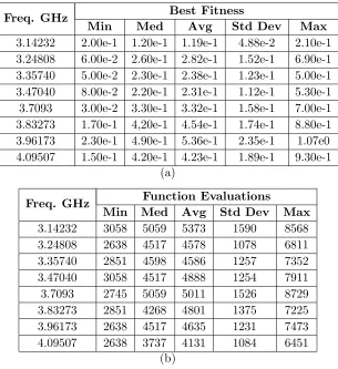
Table 8. 8-frequency SHADE statistical data.

Freq. GHz Best Fitness

Min Med Avg Std Dev Max

3.14232 6.00e-2 1.80e-1 1.65e-1 7.26e-2 2.90e-1 3.24808 6.00e-2 2.50e-1 2.61e-1 1.26e-1 5.30e-1 3.35740 7.00e-2 2.30e01 2.51e-1 1.20e-1 6.40e-1 3.47040 5.00e-2 2.20e-1 2.27e-1 9.09e-2 4.10e-1 3.7093 6.00e-2 3.40e-1 3.73e-1 1.87e-1 7.70e-1 3.83273 1.40e-1 4.70e-1 5.17e-1 2.31e-1 1.09e0 3.96173 2.50e-1 5.00e-1 5.23e-1 1.83e-1 9.60e-1 4.09507 1.40e-1 4.00e-1 3.97e-1 1.62e-1 8.00e-1

(a)

Freq. GHz Function Evaluations

Min Me Avg Std Dev Max

3.14232 2400 3900 4516 1867 9800 3.24808 2300 4300 5072 2132 10000 3.35740 2700 4000 4328 1709 10000 3.47040 2500 4500 5084 1885 10000

3.7093 2500 4400 5040 2096 9800

3.83273 2100 4700 5448 2311 10000 3.96173 2200 4400 4904 1929 10000 4.09507 2800 4200 4968 2132 10000

Table 9. 8-frequency L-SHADE statistical data.

Freq. GHz Best Fitness

Min Med Avg Std Dev Max

3.14232 2.00e-1 1.20e-1 1.19e-1 4.88e-2 2.10e-1 3.24808 6.00e-2 2.60e-1 2.82e-1 1.52e-1 6.90e-1 3.35740 5.00e-2 2.30e-1 2.38e-1 1.23e-1 5.00e-1 3.47040 8.00e-2 2.20e-1 2.31e-1 1.12e-1 5.30e-1 3.7093 3.00e-2 3.30e-1 3.32e-1 1.58e-1 7.00e-1 3.83273 1.70e-1 4,20e-1 4.54e-1 1.74e-1 8.80e-1 3.96173 2.30e-1 4.90e-1 5.36e-1 2.35e-1 1.07e0 4.09507 1.50e-1 4.20e-1 4.23e-1 1.89e-1 9.30e-1

(a)

Freq. GHz Function Evaluations

Min Med Avg Std Dev Max

3.14232 3058 5059 5373 1590 8568 3.24808 2638 4517 4578 1078 6811 3.35740 2851 4598 4586 1257 7352 3.47040 3058 4517 4888 1254 7911

3.7093 2745 5059 5011 1526 8729

3.83273 2851 4268 4801 1375 7225 3.96173 2638 4517 4635 1231 7473 4.09507 2638 3737 4131 1084 6451

(b)

18% fewer evaluations for the 5-frequency case and about 24% fewer for the 8-frequency case on the LPDA problem. L-SHADE clearly is superior to SHADE in terms of efficiency while both algorithms are similarly accurate in terms of locating optima.

4. PBM ANTENNA BENCHMARKS

The PBM benchmarks were developed to serve as a standard set of “real world” antenna problems that measure the effectiveness of an antenna optimization algorithm. They are described in detail in the Appendix. The fitness function for each problem is the antenna’s directivity which is to be maximized, that is Max [D(xi)], where the xi are decision variables specific to each problem (see Appendix for details) and where i = 1,2 for problems #1–4 and i = 1, . . . , Nel−1 for problem #5, Nel being the number of elements in a collinear array. The PBM problems do not have analytical solutions and consequently must be solved numerically. Although there are published results based on analytical solutions [36], those results are incorrect because they make several invalid assumptions, namely (i) sinusoidal current distributions, (ii) filamentary currents, and (iii) no mutual coupling between antenna elements. These assumptions are incorrect for the actual PBM antenna structures and consequently lead to incorrect results. The PBM problems can only be solved numerically.

While any numerical “modeling engine” can be used, the original PBM suite was optimized using NEC Version 2 [35], a widely available freeware version of the program developed at the Lawrence Livermore National Laboratory (US Dept. Energy). Being an MoM code, NEC is intended primarily for modeling wire structures such as the PBM benchmarks.

This paper adds SHADE and L-SHADE to the list and compares their results directly with published data. Because the modeling engine is a separate program, the optimization algorithm calls an independent NEC module that computes the fitness using decision variable values supplied by the optimizer. NEC Ver. 2 was used in the original PBM paper and here for SHADE/L-SHADE; NEC Ver. 4 was used with the other optimizers (both return the same results).

4.1. PBM Best Fitness (Maximum Directivity)

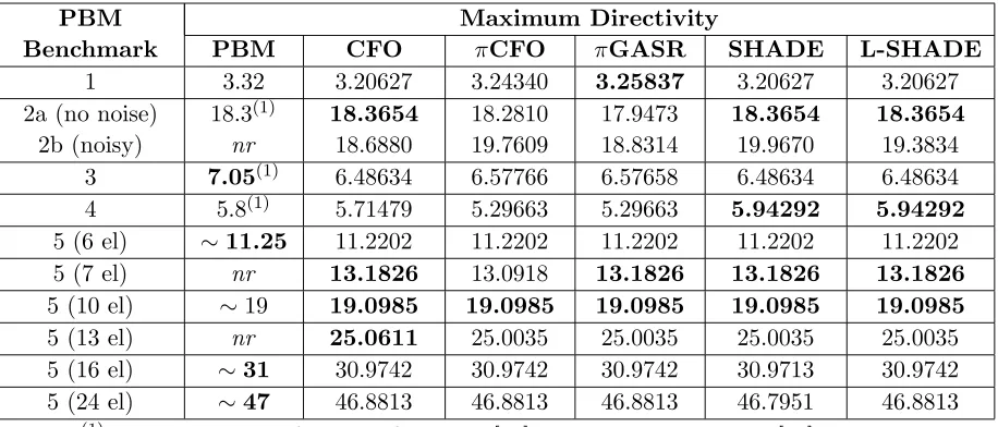
Table 10 tabulates the best fitness returned by each of the tested algorithms. Many of the PBM data are estimated from figures in the original paper and consequently carry a measure of uncertainty. The PBM data also may differ from the other optimizers’ because of subtle effects such as compiler or modeling differences, for example, source modeling in NEC. What is important is consistency in the data, and even a cursory glance at Table 10 shows the data are very consistent one algorithm to the next. With respect to how well these algorithms computed the best fitness (antenna maximum directivity), the data show that no algorithm is clearly superior. Each one returned a best fitness value that was at or close to the known maximum. The six algorithms are not distinguishable on that basis.

Table 10. Best fitness.

PBM Benchmark

Maximum Directivity

PBM CFO πCFO πGASR SHADE L-SHADE

1 3.32 3.20627 3.24340 3.25837 3.20627 3.20627

2a (no noise) 2b (noisy)

18.3(1)

nr

18.3654 18.6880

18.2810 19.7609

17.9473 18.8314

18.3654 19.9670

18.3654 19.3834

3 7.05(1) 6.48634 6.57766 6.57658 6.48634 6.48634

4 5.8(1) 5.71479 5.29663 5.29663 5.94292 5.94292

5 (6 el) ∼11.25 11.2202 11.2202 11.2202 11.2202 11.2202

5 (7 el) nr 13.1826 13.0918 13.1826 13.1826 13.1826

5 (10 el) ∼19 19.0985 19.0985 19.0985 19.0985 19.0985

5 (13 el) nr 25.0611 25.0035 25.0035 25.0035 25.0035

5 (16 el) ∼31 30.9742 30.9742 30.9742 30.9713 30.9742 5 (24 el) ∼47 46.8813 46.8813 46.8813 46.7951 46.8813 Notes: (1) values estimated from the figures in [20]; nr — not reported in [20]

values marked ∼are estimated from Fig. 13 in [20].

On PBM problem #1 SHADE and L-SHADE return the same directivity as CFO, which is a value slightly less thanπCFO’s andπGASR’s. πGASR returned the best fitness of 3.25837. On PBM #2(a) just the opposite occurred with CFO, SHADE and L-SHADE all returning a best directivity of 18.3654 while the other algorithms returned slightly lower values. Problem #2(b) is a noisy version of 2(a), details in the Appendix, whose purpose is to investigate how well the location of maximum fitness is determined, not its value because it is inherently random. This metric is discussed in connection with Table 11 which tabulates the best fitness coordinates.

On problem #3 the PBM maximum directivity of 7.05 appears suspicious because all the other optimizers returned values that are substantially lower but consistent with each other. The best value of 6.57766 is returned by πCFO with πGASR’s being very slightly less. SHADE, L-SHADE and CFO returned the same value of 6.48634. On PBM #4, SHADE and L-SHADE returned the same best fitness of 5.94292, which is better than the PBM value, and substantially higher thanπCFO’s and πGASR’s, both of which are the same.

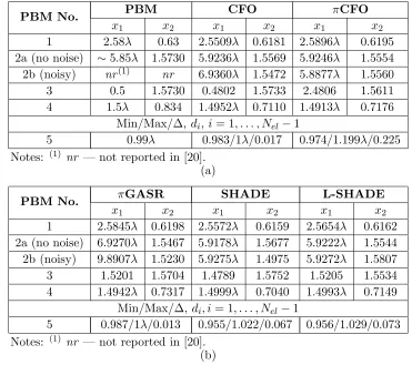
Table 11. Best fitness coordinates.

PBM No. PBM CFO πCFO

x1 x2 x1 x2 x1 x2

1 2.58λ 0.63 2.5509λ 0.6181 2.5896λ 0.6195 2a (no noise) ∼5.85λ 1.5730 5.9236λ 1.5569 5.9246λ 1.5554 2b (noisy) nr(1) nr 6.9360λ 1.5472 5.8877λ 1.5560

3 0.5 1.5730 0.4802 1.5733 2.4806 1.5611

4 1.5λ 0.834 1.4952λ 0.7110 1.4913λ 0.7176 Min/Max/Δ, d_i, i= 1, . . . , N_el−1

5 0.99λ 0.983/1λ/0.017 0.974/1.199λ/0.225 Notes: (1) nr — not reported in [20].

(a)

PBM No. πGASR SHADE L-SHADE

x1 x2 x1 x2 x1 x2

1 2.5845λ 0.6198 2.5572λ 0.6159 2.5654λ 0.6162 2a (no noise) 6.9270λ 1.5467 5.9178λ 1.5677 5.9222λ 1.5544 2b (noisy) 9.8907λ 1.5230 5.9275λ 1.4975 5.9272λ 1.5807 3 1.5201 1.5704 1.4789 1.5752 1.5205 1.5534 4 1.4942λ 0.7317 1.4999λ 0.7040 1.4993λ 0.7149

Min/Max/Δ,di, i= 1, . . . , Nel−1

5 0.987/1λ/0.013 0.955/1.022/0.067 0.956/1.029/0.073 Notes: (1) _{nr — not reported in [20].}

(b)

fractional basis. A fair reading of these data is that all six algorithms returned essentially the same maximum directivity for the variable-length collinear dipole array.

4.2. PBM Coordinates of Maximum Directivity

Locations in the decision space for the returned best fitnesses are tabulated in Table 11. Because the first four problems are two-dimensional (2D), the table lists the coordinates (x1, x2) of the computed

maximum. PBM #5, however, is (N_el−1)DwhereN_elis the number of dipole elements in the collinear array. In this case, the table lists the range of coordinate values (minimum/maximum/difference) for the computed best fitness.

On PBM #1, all algorithms returned very similar coordinates, while the PBM values are slightly different. The plots in the Appendix show a broad maximum which readily accounts for slight differences in where the optimizers placed it. For problem #2(a), the maxima locations are all quite similar except forπGASR whosex1 coordinate is significantly different than the others. This difference explains why

πGASR’s fitness in Table 10 is significantly less than the known maximum.

PBM #2(b) was included in order to investigate how well an algorithm would locate the maximum directivity’s coordinates in the presence of noise. Interestingly, their values were not reported in [20]. Each algorithm returned a similar x2 value, but their x1 values exhibit much more variability. This

effect is particularly evident in the πGASR coordinate of 9.8907λ compared to the next largest value 6.9360λreturned by CFO.

Problem #3 is interesting because its landscape is very spiky with four global maxima. All six algorithms converged on essentially the same x2 coordinate in the range 1.5534–1.5752. With respect

to x1, however, CFO and πCFO located their maxima at different x1 points, 0.4802 and 2.4806 rad,

maxima were quite similar as seen in Table 10.

On PBM #4, each algorithm performed well locating the maximum’s coordinates. The results are quite consistent with respect tox1 (known value 1.5λ). The values also are very consistent with respect

to x2 (0.7040–0.7317), but they do differ from the PBM value of 0.834.

The known coordinate for problem #5’s maximum directivity is a uniform separation of 0.99λ between collinear elements regardless of their number. Because each optimizer returns a set of separations that are not all equal, Table 11 lists the minimum and maximum values and their difference. The smaller their difference the closer the algorithm came to locating the known maximum. The tightest cluster was returned by πGASR, the loosest by πCFO. The other three optimizers returned similarly spread element separations. It is significant that in spite of the range of element separations the computed maximum array directivities in Table 10 are remarkably consistent. These data show that the collinear array’s directivity is not particularly sensitive to element separation; in other words, its maximum in the (Nel−1)D decision space is fairly broad.

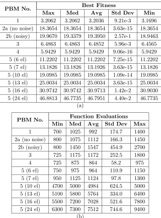
Table 12. SHADE PBM statistical data.

PBM No. Best Fitness

Max Med Avg Std Dev Min

1 3.2062 3.2062 3.2036 9.21e-3 3.1696 2a (no noise) 18.3654 18.3654 18.3654 3.63e-15 18.3654

2b (noisy) 19.9670 19.3379 19.3950 2.57e-1 18.9463 3 6.4863 6.4863 6.4852 5.96e-3 6.4565 4 5.9429 5.9429 5.9429 9.06e-16 5.9429 5 (6 el) 11.2202 11.2202 11.2202 7.25e-15 11.2202 5 (7 el) 13.1826 13.1826 13.1926 3.63e-15 13.1826 5 (10 el) 19.0985 19.0985 19.0985 1.09e-14 19.0985 5 (13 el) 25.0034 25.0034 25.0034 3.63e-15 25.0034 5 (16 el) 30.9742 30.9742 30.9713 1.42e-2 30.9030 5 (24 el) 46.8813 46.7735 46.7951 4.40e-2 46.7735

(a)

PBM No. Function Evaluations

Min Med Avg Std Dev Max

1 700 1025 992 174.7 1400

2a (no noise) 800 1075 1112 166.3 1450 2b (noisy) 800 1450 1547 454.9 2700

3 725 1175 1172 252.5 1800

4 725 875 864 58.2 975

5 (6 el) 750 975 964 110.9 1150

5 (7 el) 950 1125 1124 97.8 1300 5 (10 el) 4700 5000 4984 624.5 5000 5 (13 el) 5100 5800 5764 334.0 6400 5 (16 el) 5500 7200 7028 521.6 7800 5 (24 el) 6300 7300 7512 744.6 9400

Table 13. L-SHADE PBM statistical data.

PBM No. Best Fitness

Max Med Avg Std Dev Min

1 3.2063 3.2063 3.2033 9.24e-3 3.1670 2a (no noise) 18.3654 18.3654 18.3654 3.63e-15 18.3654

2b (noisy) 19.9764 19.3284 19.3835 2.52e-1 18.9400 3 6.4864 6.4864 6.4846 8.93e-3 6.4417 4 5.9429 5.9429 5.9429 9.06e-16 5.9429 5 (6 el) 11.2202 11.2202 11.2202 7.25e-15 11.2202 5 (7 el) 13.1826 13.1826 13.1826 3.63e-15 13.1826 5 (10 el) 19.0985 19.0985 19.0985 1.09e-14 19.0985 5 (13 el) 25.0035 25.0035 25.0035 3.63e-15 25.0035 5 (16 el) 30.9742 30.9742 30.9742 1.09e-14 30.9742 5 (24 el) 46.8813 46.8813 46.8555 4.70e-2 46.7735

(a)

PBM No. Function Evaluations

Min Med Avg Std Dev Max

1 723 1051 1031 139.3 1262

2a (no noise) 848 1081 1157 148.1 1421 2b (noisy) 865 1465 1473 329.1 2104

3 865 1302 1309 232.9 1773

4 772 1045 1021 101.2 1190

5 (6 el) 2122 2382 2385 139.3 2573 5 (7 el) 2487 2858 2868 143.4 3093 5 (10 el) 3663 4065 4046 126.6 4222 5 (13 el) 6471 6777 6822 174.6 7188 5 (16 el) 7908 8083 8110 133.8 8439 5 (24 el) 8955 9488 9446 187.8 9679

(b)

4.3. PBM Statistics

5. CONCLUSION

The SHADE and L-SHADE optimization algorithms were applied to several wire antenna problems with quite good results, specifically (i) optimal excitation of a five-element Log Periodic Dipole Array to create an omnidirectional far-field H-plane radiation pattern and (ii) optimization of the five PBM antenna benchmark problems. The algorithms’ performance was comparable to or better than that of other algorithms applied to the same problems. While both of these DE variants were comparably accurate in locating global extrema, L-SHADE was more efficient on the LPDA problem (fewer FEs), but not so on the PBM problems. The data suggest that neither algorithm is clearly more efficient for the types of wire antenna problems considered here, and which algorithm is better for a specific problem is highly dependent on the problem itself. As to the LPDA excitation problem, this work does confirm that (i) indeed it is possible to determine a set of excitations that render electromagnetically “invisible” all but one of the dipoles and (ii) that the solution is not unique. With respect to the PBM benchmarks, this work provides results that are consistent with the known solutions and comparable to other optimizers in accuracy and efficiency.

APPENDIX A. PBM BENCHMARKS

A.1 Benchmark #1: Variable Length Center-Fed Dipole

Figure A1 shows the antenna geometry for PBM problem #1. The objective function, as with all the PBM problems, is the center-fed dipole’s directivity, D, which is to be maximized as a function of its total length, L, and the polar angle, θ. A perspective view of the 2D landscape is in Fig. A2 with additional plots projecting onto the principal planes in Fig. A3. The topology or “landscape” is L= Ω∪F(X) where Ω :=X|xmin_k ≤x_k≤xmax_k , k = 1, . . . , N_dis theN_d-dimensional decision space, and F(X) : X ∈ Ω ⊂Rn _{is the fitness function being optimized. In this case it is smoothly varying} with one global maximum and two similar amplitude local maxima.

Figure A1. CF dipole.

(a) (b)

(a)

(b) (c)

Figure A3. (a) PBM #1 projected onto L-θ plane. (b) PBM #1 projected ontoθ-Dplane. (c) PBM #1 projected ontoL-Dplane.

Figure A4. PBM #2,λ/2-wave CF in-phase dipoles.

A.2 Benchmark #2: Array of Uniform Half-Wave Dipoles

PBM problem #2 is an array of uniformly spacedλ/2 dipoles (Fig. A4). All are center-fed with equal amplitude in-phase sources. Also shown is NEC’s right-handed Cartesian coordinate system polar and azimuth angles θ and φ, respectively. The objective is maximization of the directivity D(d, θ) in the plane φ = 90◦ as a function of separation d and polar angle θ with and without additive Gaussian noise. Fig. A5 shows the landscape with/without noise. Figs. A6 and A7 show principal plane plots with/without noise. Gaussian noise is generated by adding to NEC’s computed directivity a normally distributed zero-mean, 0.2-variance random variable (rv) z computed using the Box Muller method: z =μ+σ−2 ln(s) cos(2πt), where μ and σ, respectively, are the mean (0) and standard deviation (0.4472). sand tare rv’s uniformly distributed on [0,1] generated using the compiler’s internal random number generator seeded with the optimization run’s start time (seconds after midnight to the nearest 0.01 sec).

A.3 Benchmark #3: Circular Array of Half-Wave Dipoles

(a) (b)

Figure A5. (a) PBM #2 perspective view (no noise). (b) PBM #2, additive Gaussian noise.

(a)

(b) (c)

Figure A6. (a) PBM #2, no noise projected onto d-θ plane. (b) PBM #2, no noise, d-D plane. (c) PBM #2, no noise,θ-Dplane.

but the phase varies as α_n = −cos [2πβ(n−1)], n = 1, . . . ,8. The unit-amplitude excitation is V_n = cosα_n +jsinα_n. Directivity D(β, θ) in the plane φ = 0◦ is to be maximized as a function of the dimensionless parameter 0 ≤ β ≤ 4 and the polar angle θ. There are four global maxima at β_i =i−0.5, i= 1, . . . ,4; θ= π₂ (Fig. A9). Principal plane plots are shown in Fig. A10.

A.4 Benchmark #4: Vee Dipole

PBM #4 is the Vee-dipole shown in Fig. A11 comprising two equal-length arms with length Larm subtending inner angle 2α connected by a feed segment of length 2L_{f eed} excited at its midpoint. Directivity D(L_total, α) is to be maximized along the +X-axis as a function of the total length 0.5λ ≤ L_total = 2L_arm+ 2L_{f eed} ≤ 1.5λ and angle ₁₈π ≤ α ≤ π₂ (L_{f eed} = 0.01λ). Perspective views of the landscape appear in Fig. A12 with principal plane projections in Fig. A13. The Vee’s objective function is unimodal with a single global maximum atD(L_total, α) = (1.5λ,0.834) in a smoothly varying topology without pronounced local maxima.

A.5 Benchmark #5: N-Element Array of Collinear Dipoles

(a)

(b) (c)

Figure A7. (a) PBM #2 with noise,d-θplane. (b) PBM #2 with noise, d-Dplane. (c) PBM #2 with noise projected onto θ-Dplane.

Figure A8. PBM #3 circular arrayλ/2 dipoles (1λradius).

(a) (b)

(a)

(b) (c)

Figure A10. (a) PBM #3 projected ontoβ-θplane. (b) PBM #3 projected ontoβ-Dplane. (c) PBM #3 projected ontoθ-Dplane.

Figure A11. PBM #4 Vee dipole.

(a) (b)

Figure A12. (a) Vee dipole landscape, perspective view. (b) PBM #4 perspective view.

(a)

(b) (c)

Figure A13. (a) PBM #4 projected onto L-α plane. (b) PBM #4 projected onto α-D plane. (c) PBM #4 projected onto L-D plane.

Figure A14. N_el-element collinear dipole array.

REFERENCES

1. Dastranj, A., “Optimization of a printed UWB antenna: Application of the invasive weed optimization algorithm in antenna design,” IEEE Antennas & Propagation Magazine, Vol. 59, No. 1, 48–57, Feb. 2017.

2. Panduro, M. A., C. A. Brizuela, L. I. Balderas, and D. A. Acosta, “A comparison of genetic algorithms, particle swarm optimization and the differential evolution method for the design of scannable circular antenna arrays,” Progress In Electromagnetics Research B, Vol. 13, 171–186, 2009.

3. Dongho, K., J. Ju, and J. Choi, “A mobile communication base station antenna using a genetic algorithm based Fabry-P´erot resonance optimization,” IEEE Trans. Ant. & Prop., Vol. 60, No. 2, 1053, Feb. 2012.

5. Ni, T., Y.-C. Jiao, L. Zhang, and Z.-B. Weng, “Worst-case tolerance synthesis for low-sidelobe sparse linear arrays using a novel self-adaptive hybrid differential evolution algorithm,”Progress In

Electromagnetics Research B, Vol. 66, 91–105, 2016.

6. Lanza Diego, M., J. R. Perez Lopez, and J. Basterrechea, “Synthesis of planar arrays using a modified particle swarm optimization algorithm by introducing a selection operator and elitism,”

Progress In Electromagnetics Research, Vol. 93, 145–160, 2009.

7. Deb, A., J. S. Roy, and B. Gupta, “Performance comparison of differential evolution, particle swarm optimization and genetic algorithm in the design of circularly polarized microstrip antennas,”IEEE Trans. Ant. &Prop., Vol. 62, No. 8, 3920–3928, Aug. 2014.

8. Hosseini, S. A. and Z. Atlasbaf, “Optimization of side lobe level and fixing quasi-nulls in both of the sum and difference patterns by using continuous ant colony optimization (ACO) method,”

Progress In Electromagnetics Research, Vol. 79, 321–337, 2008.

9. Chang, L., C. Liao, W. Lin, L.-L. Chen, and X. Zheng, “A hybrid method based on differential evolution and continuous ant colony optimization and its application on wideband antenna design,”

Progress In Electromagnetics Research, Vol. 122, 105–118, 2012.

10. Cui, C.-Y., Y.-C. Jiao, and L. Zhang, “Synthesis of some low sidelobe linear arrays using hybrid differential evolution algorithm integrated with convex programming,”IEEE Ant.&Wireless Prop. Letters, Vol. 16, 2017.

11. Rocca, P., G. Oliveri, and A. Massa, “Differential evolution as applied to electromagnetics,” IEEE

Antennas & Propagation Magazine, Vol. 53, No. 1, 38–49, Feb. 2011.

12. Hoorfar, A., “Evolutionary programming in electromagnetic optimization: A review,”IEEE Trans. Ant. & Prop., Vol. 55, No. 3, 523–537, Mar. 2007.

13. Coleman, C. M., E. J. Rothwell, and J. E. Ross, “Investigation of simulated annealing, ant-colony optimization, and genetic algorithms for self-structuring antenna,” IEEE Trans. Ant. & Prop., Vol. 52, No. 4, 1007–1014, Apr. 2004.

14. Weile, D. S. and E. Michielssen, “Genetic algorithm optimization applied to electromagnetics: A review,”IEEE Trans. Ant. &Prop., Vol. 45, No. 3, 343–353, Mar. 1997.

15. Yerrola, A. K. and P. Spandana, “Optimization of linear antennas — A survey,” Int’l. J. Comp. App., Vol. 171, No. 3, 17–20, Aug. 2017.

16. Shan, A. and G. G. Wang, “Survey of modeling and optimization strategies to solve high-dimensional design problems with computationally-expensive black-box functions,” Struc. &

Multidisc. Opt., Vol. 41, 219–241, 2010.

17. Kuwahara, Y., “Multiobjective optimization design of Yagi-Uda antenna,” IEEE Trans. Ant. &

Prop., Vol. 53, No. 6, 1984–1992, Jun. 2005.

18. Casula, G. A., G. Mazzarella, and N. Sirena, “Evolutionary design of wide-band parasitic dipole arrays,” IEEE Trans. Ant.& Prop., Vol. 59, No. 11, 4094–4102, Nov. 2011.

19. Saraereh, O. A., A. A. Saraira, Q. H. Alsafasfeh, and A. Arfoa, “Bio-inspired algorithms applied on microstrip patch antennas: A review,” Int. J. Comm. Ant. & Prop. (I.Re.C.A.P.), Vol. 6, No. 6, 336–347, 2016.

20. Pantoja, M. F., A. R. Bretones, and R. G. Martin, “Benchmark antenna problems for evolutionary optimization algorithms,” IEEE Trans. Ant. &Prop., Vol. 55, No. 4, 1111–1121, Apr. 2007. 21. Storn, R. and K. Price, “Differential evolution: A simple and efficient adaptive scheme for global

optimization over continuous spaces,” TR-95-012, ICSI, USA, 1995.

22. Das, A., S. Mullick, and P. N. Suganthan, “Recent advances in differential evolution — An updated survey,” Swarm & Evol. Comp., Vol. 27, 1–30, 2016.

23. Zhou, X., G. Zhang, X. Hao, and L. Yu, “A novel differential evolution algorithm using local abstract convex underestimate strategy for global optimization,” Comp.&Op. Res., Vol. 75, 132– 149, 2016.

25. Tanabe, R. and A. Fukunaga, “Improving the search performance of SHADE using linear population size reduction,” Proc. IEEE Cong. Evol. Comp. 2014, 1658–1665, Beijing, 2014. 26. Liang, J., B. Qu, P. Suganthan, and A. Hernandez-Diaz, “Problem definitions and evaluation

criteria for the CEC 2013 special session and competition on real-parameter optimization,” Computational Intelligence Laboratory, Zhengzhou University, China and Technical Report, Nanyang Technological University, Singapore, 2013.

27. Liang, J., B. Qu, and P. Suganthan, “Problem definitions and evaluation criteria for the CEC 2014 special session and competition on single-objective real-parameter numerical optimization,” Computational Intelligence Laboratory, Zhengzhou University, China and Technical Report, Nanyang Technological University, Singapore, 2014.

28. Zhang, J. and C. Sanderson, “JADE: Adaptive differential evolution with optional external archive,” IEEE Trans. Evol. Comp., Vol. 13, No. 5, 945–958, 2009.

29. Isbell, D. E., “Log periodic dipole arrays,” IRE Trans. Ant. &Prop., Vol. 8, No. 3, 260–267, May 1960.

30. Jordan, E. C. and K. G. Balmain, Electromagnetic Waves and Radiating Systems, 2nd Edition, Chap. 15, Prentice-Hall, Inc., Englewood Cliffs, New Jersey, 1968.

31. Balanis, C. A.,Antenna Theory: Analysis and Design, Section 11.4, Wiley, New York, 1997. 32. Yang, J., “On conditions for constant radiation characteristics for log-periodic array antennas,”

IEEE Trans. Ant.& Prop., Vol. 58, No. 5, 1521, May 2010.

33. Lehmensiek, R. and D. I. L. de Villiers, “Optimization of log-periodic dipole array antennas for wideband omnidirectional radiation,”IEEE Trans. Ant. & Prop., Vol. 63, No. 8, 3714, Aug. 2015. 34. Lehmensiek, R. and D. I. L. de Villiers, “Constant radiation characteristics for log-periodic dipole

array antennas,”IEEE Trans. Ant. &Prop., Vol. 62, No. 5, 2966, May 2014.

35. Burke, G. J., “Numerical electromagnetics code — NEC-4.2 method of moments, Part I: User’s manual,” LLNL-SM-490875, Lawrence Livermore National Laboratory (USA), Livermore, CA, Jul. 2011.