Article
1
Source contributions to ozone formation in the New
2
South Wales Greater Metropolitan Region, Australia
3
4
Hiep Nguyen Duc1*, Lisa T.-C. Chang1, Toan Trieu1, David Salter1 and Yvonne Scorgie1
5
1 New South Wales Office of Environment and Heritage, Sydney, Australia;
6
Hiep.Duc@environment.nsw.gov.au; LisaTzu-Chi.Chang@environment.nsw.gov.au;
7
Toan.Trieu@environment.nsw.gov.au; David.Salter@environment.nsw.gov.au;
8
Yvonne.Scorgie@environment.nsw.gov.au
9
10
*Correspondence author: Hiep Nguyen Duc
11
Email: Hiep.Duc@environment.nsw.gov.au
12
Phone: +61 2 9995 5050
13
Fax: +61 2 9995 6250
14
Address: PO Box 29 Lidcombe, NSW 1825, Australia
15
16
17
Abstract: Ozone and fine particles (PM2.5) are the two main air pollutants of concern in the New
18
South Wales Greater Metropolitan Region (NSW GMR) region due to their contribution to poor air
19
quality days in the region. This paper focuses on source contributions to ambient ozone
20
concentrations for different parts of the NSW GMR, based on source emissions across the greater
21
Sydney region. The observation-based Integrated Empirical Rate Model (IER) was applied to
22
delineate the different regions within the GMR based on the photochemical smog profile of each
23
region. Ozone source contribution is then modelled using the CCAM-CTM (Cubic Conformal
24
Atmospheric Model-Chemical Transport Model) modelling system and the latest air emission
25
inventory for the greater Sydney region. Source contributions to ozone varied between regions, and
26
also varied depending on the air quality metric applied (e.g. average or maximum ozone). Biogenic
27
volatile organic compound (VOC) emissions were found to contribute significantly to median and
28
maximum ozone concentration in North West Sydney during summer. After commercial domestic,
29
power station was found to be the next largest anthropogenic source of maximum ozone
30
concentrations in North West Sydney. However, in South West Sydney, beside commercial and
31
domestic sources, on-road vehicles were predicted to be the most significant contributor to
32
maximum ozone levels, followed by biogenic sources and power stations. The results provide
33
information which policy makers can devise various options to control ozone levels in different
34
parts of the NSW Greater Metropolitan Region.
35
Keywords: Ozone; Greater Metropolitan Region of Sydney; source contribution; source attribution;
36
air quality model; Cubic Conformal Atmospheric Model (CCAM); Chemical Transport Model
37
(CTM)
38
39
1. Introduction
40
Ozone is one of the criterion pollutants monitored at many monitoring stations in the Sydney
41
metropolitan area in the past few decades (from 1970 until now). It is a secondary pollutant
42
produced from complex photochemical reaction of nitrogen oxides (NOx) and mainly volatile
43
organic compounds (VOC) under sunlight. In the metropolitan area of Sydney, NOx emissions come
44
from many different sources including motor vehicles, industrial, commercial-domestic, non-road
45
mobile (e.g. shipping, rail, aircraft) and biogenic (soil) sources. Similarly, VOC emission comes from
46
biogenic (vegetation) and various anthropogenic sources.
47
In the early 1970s until the late 1990s, ozone exceedances at a number of sites in Sydney
48
occurred frequently especially during the summer period. From early 2000 to 2010, ozone
49
concentration as measured at many monitoring stations tended to decrease. This is mainly due to a
50
cleaner fleet of motor vehicles compared to that in the past, despite an increase in the total number of
51
vehicles. Recently, there has been a slight upward trend of ozone levels in the Sydney region.
52
Controlling ozone (either maximum ozone or exposure), with least cost and best outcome, is a
53
complex problem to solve and depends on the meteorological and emission characteristics within
54
the region. A study to understand and determine the source contribution to ozone formation in
55
various parts of the Sydney metropolitan region is helpful to policy makers to manage ozone level.
56
Ozone formation from NOx and VOC under sunlight is a complex photochemical process. Sensitivity
57
of ozone concentration to changes in emission rate of VOC and NOx sources had been shown to be
58
nonlinear in many experimental and modelling studies [1].
59
Source contribution to ambient ozone concentration is important to understand the process of
60
dispersion of pollutants from various sources to a receptor point. Interests in this area, especially
61
ambient particulates, has been expanded in recent years in numerous studies on particle
62
characterisation or VOC via source fingerprints using Positive Matrix Factorisation (PMF) statistical
63
method [2-4]. Rather than a backward receptor model, a forward source to receptor dispersion
64
model can also be used to study the source contribution at the receptor point. To this end, an
65
emission inventory and an air quality dispersion model can be used to predict the pollutant
66
concentration at the receptor point, under various emission source profile scenarios, and hence can
67
isolate the source contribution of various sources [5-9].
68
Using an urban air quality model called SIRANE with tagged species approach to determine
69
the source contribution to NO2 concentration in Lyon, a large industrial city in France, Nguyen et al.
70
[9] have shown that traffic is the main cause of NO2 air pollution in Lyon.
71
Dunker et al., [5] used a set of precursors and ozone tracers to determine the source
72
contribution to ozone formation called the ozone source apportionment technology (OSAT) and
73
implemented it in the CAMx air quality model. OST allows the air quality model such as CAMx to
74
run only once and ozone formation at a receptor site can be attributed to different defined source
75
regions and different source categories within each region. They applied OSAT to study the source
76
contribution to ozone in Lake Michigan ozone study with good results as compared with using
77
sensitivity analysis using decoupled direct method (DDM) which was implemented by them before
78
in CAMx [6].
79
Li et al. [7] used CAMx with OSAT to study the source contribution to ozone in the Peral River
80
Delta (PRD) region of China. They divided the whole modelling domain including the PRD and
81
Hong Kong regions, south China region and the whole of China into 12 source areas and 7 source
82
categories which include anthropogenic sources outside PRD, biogenic, shipping, point sources,
83
areas sources such as domestic and commercial and mobile sources in PRD and in Hong Kong. Their
84
results show that under mean ozone conditions, super-regional (outside regional and PRD areas)
85
contribution is dominant but, for high ozone episodes, elevated regional and local sources are still
86
the main causative factors. Among all the sources, mobile source is the source category contributing
87
most to ozone in PRD region.
88
Wang et al. [10] used CAMx model with OSAT to study ozone source attribution during a smog
89
episode in Beijing, China. The authors showed a significant spatial distribution of ozone in Beijing
90
has strong regional contribution. Similar techniques have been used to study the source
91
apportionment of PM2.5 using source-oriented CMAQ, such as Zhang et al. [11] in their study of
92
source apportionment of PM2.5 secondary nitrate and sulfate in China from multiple emission
93
sources across China.
94
The Sydney basin with a population of more than 5 million has a diverse source of air emission
95
pattern. Beside biogenic emissions, anthropogenic source emissions such as motor vehicles and
industrial sources are two of the main contribution to ozone formation in Sydney. Duc, Spencer et
97
al. [12] used modelling approach based on a model called TAPM-CTM (The Air Pollution Model –
98
Chemical Transport Model) to show that the motor vehicle morning peak emission in Sydney
99
strongly influences the daily maximum zone level in the afternoon at various sites in Sydney,
100
especially downwind sites in the south west of Sydney.
101
Duc et al., [8] recently used CCAM-CTM (Cubic Conformal Atmospheric Model-Chemical
102
Transport Model) modelling system to determine both the PM2.5 and ozone source contribution
103
based on the Sydney Particle Study (SPS) period of January 2011. Their results show that the
104
biogenic emission contributes to about 15% to 25% to average PM2.5 and about 40% to 60% to the
105
maximum ozone at several sites in the Greater Sydney Region (GMR) during January 2011. In
106
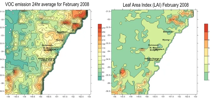
addition, the source contribution to maximum ozone at Richmond (North West Sydney) is different
107
from other sites in Sydney in that the industrial sources contribute more than mobile sources to the
108
maximum ozone at this site while the reverse is true at other sites.
109
This study extends the previous study [8] by using many additional sources including non-road
110
mobile sources (shipping, locomotives, aircrafts), commercial domestic over the whole 12 months’
111
period of 2008 and determining the source contribution of ozone for different sub-regions which
112
have different ozone characteristics in its response to NOx and VOC emission.
113
As the ozone response to NOx and VOC sources is mostly nonlinear depending on the source
114
region which is either NOx or VOC limited, the nonlinear interaction among the impacts of emission
115
sources lead to discrepancies between source contribution attributed from a group of emitting
116
sources and the sum of contribution attributed to each component [1]. For this reason, source
117
contribution is studied for the impact of each source to different regions in Sydney which is
118
characterised by base state of emission and the meteorology pattern on the regions
119
Observation-based methods can be used to provide a mean to assess the potential extent of
120
photochemical smog problem at various regions [13-14]. The Integrated Empirical Rate (IER) model,
121
developed by Johnson [14] based on the smog chamber studies, is used in this study to determine
122
and understand the photochemical smog at various regional sites in Sydney using ambient
123
measurements at the monitoring stations. The IER model have been used by Blanchard [15] and
124
Blanchard and Fairley [16] in photochemical smog studies in Michigan and California to determine
125
whether a site or a region is in a NOx-limited or VOC-limited regime.
126
Central to the IER model is the concept of smog produced (SP). Photochemical smog is
127
quantified in terms of NO oxidation which defines Smog Produced (SP) as the quantity of NO
128
consumed by photochemical processes plus the quantity of O3 produced.
129
[SP]0t [NO] [NO] [O ] [O ] 0
t t
3 t 3 0t
= − + −
130
where [NO]0t and [O ]3 0t denote the NO and O3 concentrations that would exist in the
131
absence of atmospheric chemical reactions occurring after time t=0 and [NO]t and [O3]t are the NO
132
and O3 concentrations existing at time t. [SP] 0t denotes the concentration of smog produced by
133
chemical reactions occurring during time t=0 to time t=t.
134
When there is no more NO2 to be photolysed, and no more NO to be reacted with reactive
135
organic compound to produce NO2 and nitrogen products (such as peroxyacetyl nitrate (PAN)
136
species), ozone production is stopped. This condition in photochemical process is called NOx-limited
137
regime. The ratio of the current concentration of SP to the concentration that would be present if
138
the NOx-limited regime existed is defined as the parameter “Extent” of smog production (E). The
139
extent value is indicative of how far toward attaining the NOx-limited regime the photochemical
140
reactions have progressed. When E=1, smog production is in the NOx-limited regime and the NO2
141
concentration approaches zero. When E<1, smog production is in the light-limited (or VOC-limited)
142
regime.
143
Previous study has shown that high ozone levels in the west, northwest and south west of
144
Sydney are mostly in the regime of NOx-limited while central east Sydney is mostly light-limited
145
(VOC-limited) [17]. For sensitivity analysis, it is expected that in the NOx-limited region, sensitivity
146
of ozone on NOx emission change (say per-ton) is positive while negative in the VOC-limited region.
Our study delineates the Greater Sydney Region into different sub-regions using IER method
148
and Principal Component Analysis (PCA) statistical method. Source contribution to ozone
149
formation is then determined in each of these sub-regions.
150
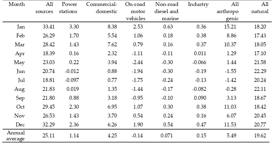
2. Methodology and data
151
2.1 CCAM-CTM Modelling system
152
The CCAM-CTM modelling system is used in this study to simulate photochemical process
153
which produce ozone over the NSW Greater Metropolitan Region (GMR). The schematic diagram of
154
CCAM-CTM, details of domain setting, model configurations as well as model validation as
155
compared to observations can be found in [18-19] of this issue of Atmosphere.
156
2.2 Emission modelling
157
The emission modelling embedded in CCAM-CTM modelling system consists of natural and
158
anthropogenic components. All natural emissions from canopy, tree, grass pasture, soil, sea salt and
159
dust are modelled and generated inline of CTM while the anthropogenic emissions is taken from the
160
EPA NSW GMR Air Emissions Inventory for calendar year 2008 and prepared offline as input to the
161
CTM.
162
The 2008 NSW GMR Air Emissions Inventory data was segregated into 17 major source groups
163
: power generation from coal, power generation from gas, residential wood heaters, on-road vehicle
164
petrol exhaust, diesel exhaust, other (e.g LPG) exhaust, petrol evaporation, non-exhaust (e.g brake)
165
particulate matter, shipping and commercial boats, industrial vehicles and equipment, aircraft
166
(flight and ground operations), locomotives, commercial non-road equipment, other
167
commercial-domestic area and industrial area fugitive sources, biogenic sources, non-biogenic
168
natural sources. Figure 1, as an example, shows the anthropogenic area source NO weekend
169
emission, motor vehicle (petrol exhaust) NO weekday emission for October 2008 and locations of
170
power stations in the GMR. The source-dependent fraction for major source groups used in emission
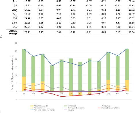
171
modelling is reference in Appendix A of [20] in this issue of Atmosphere.
172
173
175
Figure 1. Anthropogenic area source NO weekend emission (left) and motor vehicle (petrol exhaust)
176
NO weekday emission (right) for October 2008 (unit in kg/day) and locations of power stations (+) in
177
the GMR (bottom).
178
179
The emission of NOx and various species of VOC from area sources and power station point
180
sources in the GMR for a typical summer month (January 2008 weekday) is shown in Table 1. These
181
areas sources are commercial-domestic, locomotives, shipping, non-road commercial vehicles,
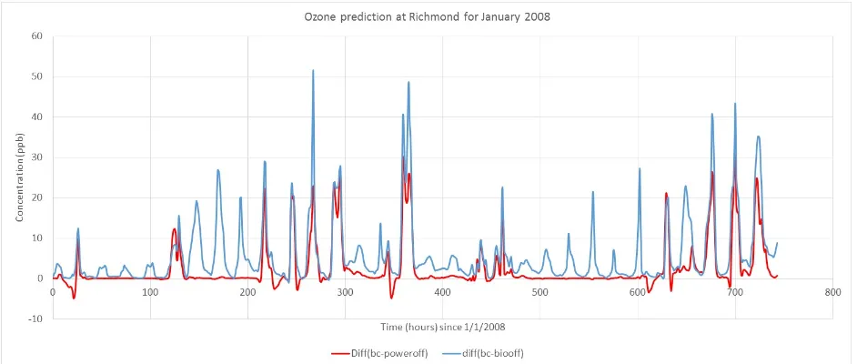
182
industrial vehicles, passenger and light-duty petrol vehicles (VPX), passenger and light-duty diesel
183
vehicles (VDX), all evaporative vehicle emission (VPV) and other vehicle exhaust (VLX).
184
185
Table 1. Emission of NOx and VOC species from various area sources in the GMR for weekday in
186
January 2008
187
188
Species (kg/h)
Commercial-
Domestic Locomotives Shipping Comm-
Veh
Ind-
Veh VPX VDX VLX VPV Power
(coal)
Power (gas) NO 4794 11450 24230 310 52197 58248 43856 502 0 121957 1681
NO2 387 924 1955 25 4213 3653 10501 31 0 6036 89
ALD2 4527 57 784 6 741 841 280 39 5768 30 9
ETH 1631 159 503 9 1208 3167 303 150 0 0 11
FORM 785 47 197 9 1027 561 454 26 435 1 73
ISOP 2 0 0 0 0 12 7 1 19 0 0
OLE 2094 43 421 3 336 1506 122 72 626 21 20
PAR 94905 291 14195 22 2283 10867 1915 518 46536 583 287
TOL 14480 24 3615 4 301 3523 172 167 1693 44 0
XYL 16495 22 4851 4 244 3997 494 190 1048 120 0
ETOH 22714 0 11 0 1 70 0 0 200 0 0
MEOH 4067 0 27 0 5 51 55 2 0 0 0
189
The biogenic emission is modelled and generated inline in CTM. For ozone, the main biogenic
190
contribution (VOC, NOx and NH3) is from vegetation and soil. The biogenic VOC is the sum of these
191
species, isoprene, monoterpene, ethanol, methanol, aldehyde and acetone.
192
The biogenic emission consists of emission from forest canopies, pasture and grass and soil. The
193
canopy model divides the canopy into an arbitrary number of vertical layers (typically 10 layers are
194
used). Biogenic emissions from a forest canopy can be estimated from a prescription of the leaf area
195
index, LAI (m2 m-2), the canopy height hc (m), the leaf biomass Bm (g m-2), and a plant
196
genera-specific leaf level VOC emission rate Q (µg-C g-1 h-1) for the desired chemical species. The
197
LAI used in CTM is based on Lu et al [21] scheme which consists of LAI for tree and grass derived
198
from Advanced Very High Resolution Radiometer (AVHRR) normalized difference vegetation
199
index (NDVI) data between 1981 and 1994.
Biogenic NOx emission model from soil is based on the temperature-dependent equation (1).
201
Q = Q noxexp[0.71(T - 30)] (1)
202
where Qnox is the
NO
x emission rate at 30°C and T is the soil temperature (°C).203
Ammonia (NH3) emission is based on Battye and Barrows scheme [22]. This approach uses
204
annual average emission factors prescribed for four natural landscapes (forest, scrubland,
205
pastureland, urban).
206
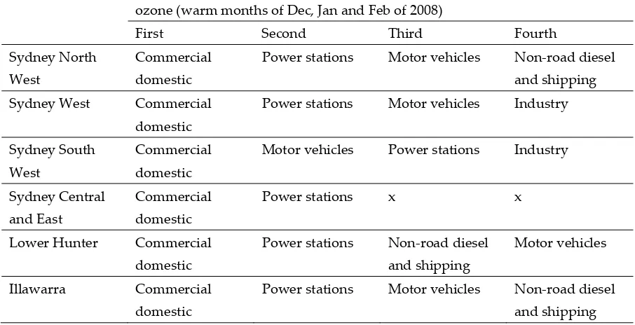
207
Figure 2. VOC monthly 24 hourly average emission (kg/hour) (left) and Leaf Area Index (LAI)
208
(right) for February 2008.
209
210
Biogenic VOC is defined as the sum of isoprene, monoterpene, ethanol, methanol, aldehyde
211
and acetone. As shown in Figure 2, biogenic VOC emission occurs mostly in west of Sydney and
212
Blue Mountain area, the National Park areas in the north, the lower Hunter and the inland of the
213
Illawarra escarpment. Isoprene and monoterpene in general have similar spatial patterns as VOC
214
distribution and reflect the Leaf Area Index (LAI) distribution in the modelling domain [8]
215
2.3 Emission scenarios
216
The 2008 NSW GMR Air Emissions Inventory data is segregated into 16 major source groups
217
then re-grouped in to 8 categories which are similar to those used by Karagulian, Belis et al. [23] to
218
match with the six identified categories using the component profile of the European Guide on Air
219
Pollution Source Apportionment with Receptor Models for particles [24]. The emissions scenarios
220
used in this study are: 1. All sources; 2. All anthropogenic – with emissions from all anthropogenic
221
sources; 3. All natural - with emissions from all natural sources; 4. Power stations: emissions from
222
coal and gas power generations; 5. On-road motor vehicles: emissions from petrol exhaust, diesel
223
exhaust, other exhaust, petrol evaporative and non-exhaust particulate matter; 6. Non-road diesel
224
and marine: with emissions from shipping and commercial boats, industrial vehicles and
225
equipment, aircraft, locomotives, commercial non-road equipment; 7. Industry: with emissions from
226
all point source except power generations from coal and gas; 8. Commercial-domestic: with
227
emissions from commercial and domestic-commercial area source excluded solid fuel burning
228
(wood heaters).
229
2.4 Source attribution to ozone formation in different sub-regions
230
Using 2008 summer (November 2007 to March 2008) observed hourly monitoring data (NO,
231
NO2, Ozone and Temperature) in the IER method, the extent of photochemical smog production in
232
various Sydney sites is determined and then classified using clustering statistical method. At low
233
level of pollutant concentrations, near background levels, with little or no photochemical reaction,
234
the extent can be equal to 1. For this reason, to better classify the degree of photochemical reaction,
235
the ozone level or the SP (smog produced) concentration has to be taken into account in addition to
236
the extent variable.
It is therefore more informative to categorise the smog potential using both the extent value and
238
the ozone concentration such as
239
- category A : extent > 0.8 and ozone conc. > 7 pphm
240
- category B : 0.5 < extent < 0.8 and 5pphm < ozone conc. < 7 pphm
241
- category C : 0.5 < extent < 0.8 and 3 pphm < ozone conc. < 5 pphm
242
- category D : extent > 0.9 and ozone conc. < 3 pphm
243
Category A represents very high ozone episode, category B high ozone episode, category C
244
medium smog potential and category D as background or no smog production.
245
Using similar techniques as those of Yu and Chang [25], the principal component analysis
246
(PCA) via correlation matrix on the 2007/2008 (1/11/2007 to 31/3/2008) summer ozone data is then
247
used to delineate the regions in the Sydney area.
248
3. Results
249
3.1 Regional delineation using Integrated Empirical Rate (IER) model and Principal component analysis
250
(PCA)
251
The delineation of sub-regions in the GMR region based on their similar ozone formation
252
patterns are performed using clustering method and PCA method. These methods produce similar
253
results. We present here the PCA results with component scores which show that there are 3
254
principle components explaining most of the variances. The eigenvalues of the correlation matrix
255
and the corresponding principal component scores for each site are derived. The contour plot of
256
component scores for each component is used to delineate the regions.
257
The main sub-regions are western Sydney (North West, West, South West) and the coastal
258
region consisting of eastern Sydney, Lower Hunter and the Illawarra as shown in Figure 3a. The
259
patterns of sub-regional delineation are similar to those that was performed for summer 1997/1998
260
[26-27] as depicted in Figure 3b. This means that over the past 20 years the spatial pattern of ozone
261
formation does not show much change.
264
(a) Chullura Newcastle Wollongong Richmond Albion Park Beresfield Bringelly Lindfield Randwick StMarys Bargo Oakdale Kembla Grange200 250 300 350 400 450 500
6150 6200 6250 6300 6350 6400 6450 Pacific Ocean Principle component 1 score contour (summer 2007/2008)
Chullura Newcastle Wollongong Richmond Albion Park Beresfield Bringelly Lindfield Randwick StMarys Bargo Oakdale Kembla Grange
200 250 300 350 400 450 500
6150 6200 6250 6300 6350 6400 6450 Pacific Ocean Principle component 2 score contour (summer 2007/2008)
0.5 Chullura Newcastle Wollongong Richmond Albion Park Beresfield Bringelly Lindfield Randwick StMarys Bargo Oakdale Kembla Grange
200 250 300 350 400 450 500 6150 6200 6250 6300 6350 6400 6450 Pacific Ocean Principle component 3 score contour (summer 2007/2008)
0.5 Chullura Newcastle Wollongong Richmond Albion Park Beresfield Bringelly Lindfield Randwick StMarys Bargo Oakdale Kembla Grange
200 250 300 350 400 450 500
6150 6200 6250 6300 6350 6400 6450 Pacific Ocean Photochemical smog regions for summer 2007/2008
(b)
200 250 300 350 400 450 500
6150 6200 6250 6300 6350 6400 6450 2 2 New 3 Wol 3 Ric 2 3 Alb 3 Ber 2 2 1 1 3 3 3 1 1 1 3 Wal 3 War 3 Bar 2 Oak 1 Pacific Ocean Principal component 1 score contour
200 250 300 350 400 450 500
200 250 300 350 400 450 500 6150 6200 6250 6300 6350 6400 6450 2 2 New 3 Wol 3 Ric 2 3 Alb 3 Ber 2 2 1 1 3 3 3 1 1 1 3 Wal 3 War 3 Bar 2 Oak 1 Pacific Ocean Principal component 3 score contour
200 250 300 350 400 450 500
6150 6200 6250 6300 6350 6400 6450 2 2 New 3 Wol 3 Ric 2 3 Alb 3 Ber 2 2 1 1 3 3 3 1 1 1 3 Wal 3 War 3 Bar 2 Oak 1 Pacific Ocean Ozone regions
265
Figure 3. Contour plots of first 3 principal component scores depicting the regional delineation
266
based on similarity of ozone formation pattern in (a) 2007/2008 and in (b) 1997/1998. The last plot in
267
each graph is the combined plots of the 3 component score contours.
268
269
From the PCA analysis showing the spatial pattern of ozone formation, the Lower Hunter and
270
Illawarra can be considered as separate from Sydney and the Sydney western region is separate
271
from eastern and central Sydney. The western Sydney region is characterised by having high
272
frequency of smog events (NOx-limited or extent of smog production higher than 0.8) as shown in
273
Table 2 of number of observed hourly data that are classified in each of the 4 smog potential
274
categories for January 2008. Sites near the coast such as Randwick and Rozelle are in VOC-limited
275
area with low smog events (zero number of observed hourly data in category A and category B).
276
277
Table 2. Number of observed hourly data that are classified into each smog potential categories at
278
different sites in the GMR for January 2008
279
Site Category A Category B Category C Category D
Randwick 0 0 12 1431
Rozelle 0 0 38 215
Lindfield 0 8 88 414
Liverpool 6 5 83 198
Bringelly 12 3 46 1138
Chullora 3 7 92 214
Earlwood 0 7 68 300
Wallsend 0 2 52 2060
Newcastle 0 0 1 597
Beresfield 0 0 26 598
Wollongong 0 1 24 797
Kemble Grange 0 0 53 1437
Richmond 4 1 9 863
Bargo 8 0 9 1061
St Marys 12 1 46 756
Vineyard 1 0 14 763
Prospect 13 2 62 225
McArthur 15 4 60 788
Oakdale 13 0 11 2007
Albion Park South 0 2 47 1441
The Sydney western region is also sub-divided into 3 sub-regions, northwest Sydney, west
281
Sydney and southwest Sydney as the northwest is also influenced by sources in the Lower Hunter
282
and the southwest is related to some extend the Illawarra region as shown by PCA analysis. The
283
results confirm previous studies [17], [25-26] which have shown that the GMR region can be divided
284
into sub-regions (north west, south west, west and central east) based on the ozone smog
285
characteristics formed from the influence of meteorology and emission pattern in the GMR.
286
The GMR region are therefore can be divided into 6 sub-regions for ozone source contribution
287
study: Sydney North West, Sydney South West, Sydney West, Central and East Sydney, the
288
Illawarra in the south and the Lower Hunter region in the north.
289
290
3.2 Source contribution to ozone over the whole GMR region
291
The CCAM-CTM predicted daily maximum 1-hour and 4-hour ozone concentrations in the
292
GMR domain (9 km x 9 km) for the entire calendar year of 2008 under various emission scenarios are
293
extracted at grid point nearest to the location of the 18 NSW OEH air quality monitoring stations.
294
Results from maximum 1-hour and 4-hour ozone analysis are very similar, therefore only results for
295
1-hour predicted maximum ozone are presented.
296
Table 3 and Figure 4 shows the average source contributions to daily maximum 1-hour ozone
297
over the whole GMR. Apparently, natural sources are more significant in contributing to ozone
298
concentration than all anthropogenic sources. During summer months (December, January and
299
February), commercial domestic, power stations and on-road motor vehicles sources contribute
300
most to ozone formation in that order. During winter months (Jun, July and August), most of
301
anthropogenic sources contribute negatively to ozone formation (i.e. the presence of these sources
302
decreases the level of ozone). Of anthropogenic sources beside commercial domestic sources, power
303
stations contribute more to ozone formation within whole GMR than that contributed from on-road
304
motor vehicle, industrial and non-diesel and marine sources in this order.
305
306
Table 3. Monthly average of daily maximum 1-hour predicted ozone concentration (ppb) in the
307
GMR for different months in 2008 under various emission scenarios
308
309
Month All
sources
Power stations
Commercial- domestic
On-road motor vehicles
Non-road diesel and marine
Industry All anthropo
genic
All natural
Jan 33.41 3.30 8.38 2.53 0.63 0.36 15.21 18.20
Feb 26.29 1.70 5.54 1.06 0.18 0.38 8.86 17.43
Mar 28.42 1.43 7.62 0.79 0.16 0.37 10.37 18.05
Apr 18.39 0.16 2.32 -1.11 -0.11 0.011 1.29 17.10
May 23.03 0.22 3.94 -2.44 -0.30 -0.066 1.44 21.58
Jun 20.74 -0.012 0.88 -1.94 -0.30 -0.19 -1.55 22.29
Jul 18.81 -0.097 0.77 -1.75 -0.24 -0.13 -1.42 20.24
Aug 21.83 0.019 1.35 -1.44 -0.17 -0.082 -0.28 22.11
Sep 21.80 0.88 3.18 -0.95 -0.10 0.090 3.13 18.67
Oct 29.45 2.30 6.95 1.07 0.30 0.38 11.03 18.42
Nov 26.53 1.43 3.70 0.54 0.24 0.16 6.07 20.45
Dec 32.29 2.36 6.26 1.90 0.54 0.47 11.53 20.77
Annual
average 25.11 1.14 4.25 -0.14 0.071 0.15 5.49 19.62
311
Figure 4. Contribution of all anthropogenic and natural emissions (bar graph) and different
312
anthropogenic sources (line graph) to the monthly average of daily maximum 1-hour ozone
313
concentration in 2008 in the GMR.
314
315
The monthly average of daily maximum 1-hour ozone concentration for January 2018 for the 4
316
emission scenarios: base case, commercial-domestic sources off, power stations sources off and
317
on-road mobile sources off is shown in Figure 5. The spatial pattern in daily maximum 1-hour ozone
318
from various source contribution is not uniform across the GMR as expected. The spatial pattern of
319
maximum 1-hour ozone shows that the relative importance of source contribution is different for
320
different sub-regions.
321
322
(a) (b)
Figure 5. Monthly average of daily maximum 1-hour ozone concentration for January 2018 in (a)
323
base case, (b) commercial-domestic sources off, (c) power stations sources off and (d) on-road mobile
324
sources off emission scenarios
325
3.3 Source contribution to ozone concentrations over sub-regions within GMR
326
The daily maximum 1-hour and 4-hour predicted ozone concentrations under various
327
emission scenarios are further analysed in this section to investigate the source contributions to
328
ozone formation in each of the sub-regions across GMR for the year of 2008. As shown above from
329
PCA analysis, the different sub-regions have different smog characteristics as represented by the
330
extent of smog production or NOx/VOC relationship with ozone level production. The 6 regions of
331
the GMR are Sydney north-west (Richmond and Vineyard), Sydney west (Bringelly, Prospect and St
332
Marys), Sydney south-west (Bargo, Liverpool and Oakdale), Sydney east (Chullora, Earlwood,
333
Randwick and Rozelle), Illawarra (Albion Park, Kembla Grange and Wollongong) and Lower
334
Hunter or Newcastle (Newcastle) regions. As for the whole GMR region analysis, only results for
335
1-hour predicted ozone are presented here since the 4-hour ones are very similar.
336
3.3.1 Sydney north-west region
337
This region is characterised as mostly NOx-limited during ozone season (summer). Table 4 and
338
Figure 6 show that, of the anthropogenic sources, commercial domestic sources (except wood
339
heaters) contribute most to the 1-hour ozone max, especially in the summer months. Then power
340
stations and motor vehicles are next in importance in contribution to ozone in the north west.
341
Interestingly, during cold winter months, on-road motor vehicles have a negative contribution to
342
maximum 1-hour ozone in the northwest of Sydney (i.e., increase in motor vehicle emission actually
343
decreases the maximum ozone level in that region). This is due to the fact that photochemical ozone
344
production never or rarely reach NOx-limited during daytime, that is it is mostly in light-limited (or
345
VOC-limited) regime everywhere in the basin.
346
Table 4. Monthly average of daily maximum 1-hour ozone concentration (ppb) in the Sydney
347
north-west region for different months in 2008 under various emission scenarios
348
Month All
sources
Power stations
Commercial -domestic
On-road motor vehicles
Non-road diesel and marine
Industry
All anthropo
genic
All natural
Jan 26.26 2.72 4.39 1.29 0.49 0.22 9.11 17.15
Feb 21.81 1.39 3.29 0.28 0.15 0.15 5.26 16.54
Mar 23.27 1.15 4.95 -0.28 0.11 0.14 6.08 17.19
Apr 16.01 0.09 1.59 -1.51 -0.20 -0.11 -0.12 16.13
Jun 17.57 -0.08 0.58 -2.77 -0.37 -0.26 -2.89 20.46
Jul 15.81 -0.16 0.48 -2.46 -0.29 -0.18 -2.61 18.42
Aug 19.02 -0.07 0.97 -1.94 -0.24 -0.16 -1.40 20.42
Sep 18.67 0.44 2.33 -1.36 -0.19 -0.04 1.20 17.47
Oct 24.49 2.00 4.48 0.23 0.21 0.23 7.17 17.32
Nov 22.25 1.15 2.40 -0.10 0.15 0.09 3.69 18.56
Dec 26.54 1.99 3.29 1.02 0.41 0.30 7.00 19.54
Annual
average 20.91 0.90 2.64 -0.90 -0.01 0.01 2.65 18.26
349
350
Figure 6. Contribution of all anthropogenic and natural emissions (bar graph) and different
351
anthropogenic sources (line graph) to the monthly average of daily maximum 1-hour ozone
352
concentration in 2008 in the Sydney north-west region
353
To examine in details the change in ozone level, Figure 7 shows difference in predicted 1-hour
354
ozone (ppb) at Richmond for January 2008 between base case and for scenarios when no biogenic
355
emissions is present and when there is no emission from power station. Biogenic emission
356
significantly increases the ozone level and is the most important source contribute to ozone
357
maximum. Power station emission from neighbouring region in the Lower Hunter also strongly
358
influences the 1-hour maximum ozone level in Sydney north-west as also shown in Figure 7. Note
359
that, at night, ozone level is higher than the base case when coal-gas power station emissions are off
360
as there is less NOx emission to scavenge the ozone
361
To be able to summarise the whole distribution of predicted ozone with minimum, maximum,
362
median values, Figure 8 shows the box plots of ozone prediction for January 2008 under different
363
emission scenarios.
367
368
369
Figure 7. Time series of difference in predicted 1-hour ozone (ppb) at Richmond for January 2008
370
between base case and biogenic emissions off (blue) and between base case and power stations
371
emissions off (red)
372
373
374
Figure 8. Box plot for 1-hour ozone concentration (ppb) in January 2008 under different emission
375
scenarios at Richmond.
376
377
3.3.2 Sydney west, Sydney south-west, Sydney east regions
378
In the Sydney west region, the on-road motor vehicle emission has slightly more contribution to
379
ozone 1-hour max than that from power stations in the summer months. But during cooler months
in autumn and winter, motor vehicle has a negative contribution to daily maximum 1-hour ozone
381
level
382
Appendix A shows the tables and graphs summarising the effect of each source to the ozone
383
formation in each of the regions.
384
In the Sydney south-west region, which is mostly in NOx-limited during ozone season and is
385
downwind from Sydney central east region, the on-road motor vehicle emission has more
386
contribution to daily maximum 1-hour ozone than that from power stations in the summer months.
387
Next is industry and then non-diesel and shipping sources in that order as ranked contribution to
388
ozone concentration.
389
In Sydney east region, the motor vehicle emission, on average for each month, contributes
390
negatively to the 1-hour maximum ozone concentration in all months of the year 2008 in this region
391
(as represented by the 3 sites listed above). As this region is in light-limited regime (or VOC-limited),
392
an increase in NOx emission from motor vehicle sources will reduce the ozone level.
393
As shown in Figure A.6 (Appendix) of the box plots of ozone concentration at Chullora for
394
January 2008, even though the monthly maximum is reduced when mobile source is turned off but
395
the median ozone increased slightly. This is because the night time ozone increases when there is
396
less NOx emission to scavenge the ozone. Ozone level also increases during day time, when ozone
397
level is low and in the VOC-limited photochemical process, if NOx emission is decreased. This can
398
be seen in the time series of difference in predicted ozone levels at Chullora for January 2008 under
399
base case and no motor vehicle emission scenario as shown in Figure 9. Maximum ozone is reduced
400
for days where the ozone is high but, for days when ozone is low and at night, ozone level is higher
401
when motor vehicle emission is turned off. The time series shows that Chullora, most of the time
402
during January 2008, is in in VOC-limited regime. Also shown in Figure 9 is the time series of
403
difference in predicted ozone under base case and when no power station emission present. Higher
404
level of local NOx due to emission from motor vehicle compared to that received downwind from
405
power station has a more dramatic effect on ozone level at Chullora.
406
407
408
409
Figure 9. Time series of difference in predicted 1-h ozone (ppb) at Chullora for January 2008 between
410
base case and motor vehicle emissions off (red) and between base case and power station emission
411
off (blue)
412
413
3.3.3 Illawarra and Lower Hunter regions
414
In the Illawarra region, after commercial domestic sources, power stations and motor vehicles
415
are next in importance in contribution to ozone formation. However, in Lower Hunter (Newcastle)
416
region, of anthropogenic contribution, power stations, non-road diesel and shipping sources are
417
more important than motor vehicle and industrial sources (see Appendix A).
419
Table 7 summarises the order of importance in source contribution to 1-hour ozone maximum in
420
each of the 6 sub-regions of the GMR Sydney region.
421
422
Table 7. Ranked order of contribution from anthropogenic sources to maximum 1-h ozone (warm
423
months). For Central and East Sydney, motor vehicle or industry emission decreases the maximum
424
1-hour ozone (negative contribution) and is denoted by x in the table.
425
426
Region Ranked order of contribution from anthropogenic sources to maximum 1-h
ozone (warm months of Dec, Jan and Feb of 2008)
First Second Third Fourth
Sydney North
West
Commercial
domestic
Power stations Motor vehicles Non-road diesel
and shipping
Sydney West Commercial
domestic
Power stations Motor vehicles Industry
Sydney South
West
Commercial
domestic
Motor vehicles Power stations Industry
Sydney Central and East
Commercial domestic
Power stations x x
Lower Hunter Commercial
domestic
Power stations Non-road diesel
and shipping
Motor vehicles
Illawarra Commercial
domestic
Power stations Motor vehicles Non-road diesel
and shipping
427
4. Discussion
428
Air quality models have been used recently to study the source contribution to air pollution
429
concentration at a receptor by various authors. The main models that are currently used are the
430
source-oriented CMAQ model and the CAMx model with OSAT. The main advantage of these
431
models are that they treated emitted species from different sources separately and hence can identify
432
source contributions to ozone in a single model run rather than multiple runs by the chemical
433
transport models (CTM) using brute force method as used in this study [7].
434
Caiazzo et al [28], in their study of quantifying the impact of major sector on air pollution and
435
early deaths in the whole US in 2005 using WRF/CMAQ model, estimated that ~10,000 (90% CI:
436
-1,000 to 21,000) premature deaths per year due to changes in maximum ozone concentrations. The
437
largest contributor for early deaths due to increase in maximum ozone is road transportation with
438
~5,000 (90% CI: -900 to 11,000) followed by power generation with ~2000 (90% CCCCI: -300 to 4000)
439
early deaths per year.
440
Our study on source contribution to ozone formation in the Greater Metropolitan Region
441
(GMR) of Sydney in 2008 has identified biogenic sources (mainly vegetation via isoprene and
442
monoterpene emission) is the major contributor to ozone formation in all regions of the GMR. This
443
result confirms the previous study of Duc et al. [8] on ozone source contribution in the Sydney
444
Particle Study (SPS) period of January 2011. Similarly, Ying and Krishnan [29] in their study of
445
source contribution of VOC in southeast Texas based on simulation using CMAQ model have found
446
for maximum 8-hour ozone occurrences from 16 August to 7 September 2000., the median of relative
447
contributions from biogenic sources was approximately 60% compared to 40% of anthropogenic
448
ones. As biogenic emission is a major contribution to ozone formation, it is important for model to
449
account it as accurate as possible. Emmerson et al. [30] has found that the Australian Biogenic
450
Canopy and Grass Emission Model (ABCGEM), as implemented in the current CCAM-CTM model
used in this study, accounts for biogenic VOC emission (especially monoterpenes) from Australian
452
eucalyptus vegetation better than The Model of Emissions of Gases and Aerosols from Nature
453
(MEGAN) when compared these modelled emissions with observations.
454
Among the anthropogenic sources, commercial and domestic sources are the main contributors
455
to ozone concentration in all regions. While power station or motor vehicles sources, depending on
456
the regions, are the next main contributors of ozone formation. In the cooler months, these sources
457
(power stations and motor vehicles) instead decrease the level of ozone. From Table 1, commercial
458
domestic sources (except wood heaters) have much higher emission of most VOC species than other
459
sources even though they emitted less NOx than other mobile sources. For this reason, it is not
460
surprising that commercial and domestic sources contribute most to the ozone formation in all the
461
metropolitan regions.
462
As it is not possible or practical to control biogenic emission sources, the implication of this
463
study is that to control the level of ozone in the GMR, the commercial and domestic sources should
464
be the focus for policy makers to manage the ozone level in the GMR. As shown in Figure 5, when
465
commercial domestic sources are turned off, a reduction in ozone is attained in all regions in the
466
GMR.
467
A reduction in power station emission will significantly improve the ozone concentration in the
468
north west of Sydney but less so in other regions of the GMR. Gégo et al. [31] in their study of the
469
effects of change in nitrogen oxides emissions from the electric power sector on ozone levels in
470
eastern U.S using CMAQ model for the 2002 model year, have shown that ozone concentrations
471
would have been much higher in much of the eastern United States if NOx emission controls had not
472
implemented by the power sector and exceptions occurred in the immediate vicinity of major point
473
sources where increased NO titration tends to lower ozone levels.
474
Motor vehicle is less a problem compared to commercial domestic and power station sources
475
except for the south west of Sydney. However, south west of Sydney has more smog episodes than
476
other regions in the GMR, therefore, to reduce high frequency of ozone events, control of motor
477
vehicle emission should be given more priority than control of emission from power station sources.
478
As shown in Figure 5, a significant reduction of ozone in the southwest compared to other regions is
479
achieved when on-road mobile sources were turned off. This region is downwind from the urban
480
area of Sydney where the largest emission source of NOx and VOC precursors is motor vehicle and
481
hence will cause elevated ozone downwind in the south west of Sydney. Various studies have
482
shown that areas downwind from the upwind emission of precursors experience high ozone [32-33].
483
Li, Lau et al. [7] showed that ozone in upwind area of the Pearl River Delta in China is mostly
484
affected by super-regional sources and local sources while downwind area has higher ozone and is
485
affected by regional sources in its upwind area beside the super-regional and local source
486
contribution.
487
It should be noted that our results on the source contribution to ozone is only applied to the
488
base 2008 emission inventory data. If this “base state” of emission is changed to a different
489
composition of VOC and NOx emissions (such as the 2013 or 2018 emission inventories), then the
490
source contribution results could be different as the relation of ozone formation with VOC and NOx
491
precursors emissions at various regions in the GMR is nonlinear and complex.
492
As ozone response to emitting sources of VOC and NOx is nonlinear, the contribution of each
493
source to maximum ozone is depending on the “base state” consisting of all other emitting sources
494
in the region. Uncertainty in the emission inventory of these sources therefore also affects the
495
contribution of ozone attributed to this source. Cohan et al. [1] has shown that underestimates of
496
NOx emission rates lead to underprediction of total source contribution but overprediction of
497
per-ton sensitivity.
498
Fujita et al. [34] in their study of source contributions of ozone precursors in California’s South
499
Coast Air Basin to ozone weekday and weekend variation had shown that reduced NOx emission of
500
weekend emission from motor vehicle caused higher level of ozone than during the weekday due to
501
the higher ratio of NMHC (Non-methane Hydrocarbon) to NOx in this VOC-limited basin.
It is therefore important to determine and understand which region in the GMR is NOx-limited
503
or VOC-limited. The observation-based IER method which uses monitoring station data is proved to
504
be useful in delineation different regions of photochemical smog profiles within the GMR where
505
monitoring stations are located. Based on the results from IER method, the results of source
506
contribution to maximum ozone in the GMR using air quality model for different emission scenarios
507
can be understood and explained adequately from emission point of view and therefore facilitate
508
policy implementation.
509
As for policy implementation in reducing ozone, it should be pointed out that even though
510
Sydney ozone trend in the past decade has decreased but background ozone trend is actually
511
increasing [35] which is part of a world-wide trend of increasing background level in many areas of
512
the world. This will make the reduction of ozone further in the future much more difficult such as
513
shown and discussed by Parrish et al. [36] in their study of background ozone contribution to the
514
California air basins.
515
5. Conclusions
516
This study provides a detailed source contribution to ozone formation in different regions of the
517
Greater Metropolitan Regions of Sydney. The importance of each source in these regions is
518
depending on the ozone formation potential of each of these regions and whether they are in
519
NOx-limited or VOC-limited photochemical regime in ozone season. Extensive monitoring data
520
available from the OEH monitoring network and many previous studies using observation-based
521
method have provided an understanding of the ozone formation potential in various sub-regions of
522
the GMR.
523
Biogenic emission is the major contributor to ozone formation in all regions of the GMR due to
524
their large emission of VOC. Of anthropogenic emission, commercial and domestic sources are the
525
main contributors to ozone concentration in all regions. These commercial domestic sources (except
526
wood heaters) have much higher emission of most VOC species but less NOx than other sources such
527
as mobile sources and hence contribute more to the ozone formation in all the metropolitan regions
528
compared to others. The commercial and domestic sources should be the focus for policy makers to
529
manage the ozone level in the GMR
530
While power station or motor vehicles sources, depending on the regions, are the next main
531
contributors of ozone formation, in the cooler months, these sources (power stations and motor
532
vehicles) instead decrease the level of ozone.
533
In the north west of Sydney, a reduction in power station emission will significantly improve
534
the ozone concentration there.
535
Motor vehicle is less a problem compared to commercial domestic and power station sources
536
except for the south west of Sydney. As the south west of Sydney has more smog episodes than other
537
regions in the GMR, control of motor vehicle emission should be given more priority than control of
538
emission from power station sources to reduce high frequency of ozone events in the Sydney basin.
539
Our next study in relation to source contribution to ozone formation will focus on the health
540
impact of each emission source on various health endpoints from their contribution to poor air
541
quality (e.g. ozone and PM2.5) in the GMR.
542
.
543
Acknowledgments: Open access funding for this work is provided from the Office of Environment & Heritage,
544
New South Wales (OEH, NSW).
545
546
Author Contributions:
547
Conceptualization, Hiep Duc.; methodology, Hiep Duc, Lisa T.-C. Chang.; software, Hiep Duc, Toan Trieu,
548
David Salter; validation, Lisa T.-C. Chang, Toan Trieu and David Salter; formal analysis, Hiep Duc.;
549
investigation, Hiep Duc, Lisa T.-C. Chang; resources, Hiep Duc, David Salter, Yvonne Scorgie; data curation,
550
Hiep Duc, Lisa T.-C. Chang, Toan Trieu, David Salter; writing—original draft preparation, Hiep Duc.;
writing—review and editing, Hiep Duc, Lisa T.-C. Chang; visualization, Hiep Duc, Lisa T.-C. Chang;
552
supervision, Hiep Duc; project administration, Yvonne Scorgie.; funding acquisition, Clare Murphy.
553
Funding: This research received no external funding except support from Clean Air and Urban Landscapes
554
(CAUL) Research Hub for retreat conference.
555
Conflicts of Interest: The authors declare no conflict of interest.
References
558
1. Cohan, D.; Hakami, A.; Hu, Y.; et al. Nonlinear Response of Ozone to Emissions: Source Apportionment
559
and Sensitivity Analysis, Environ. Sci. Technol., 2005, 39 (17): 6739–6748.
560
2. Buzcu, B.; Fraser, M. Source identification and apportionment of volatile organic compounds in
561
Houston, TX, Atmospheric Environment, 2006, 40, 13:2385-2400,
562
https://doi.org/10.1016/j.atmosenv.2005.12.020
563
3. Ling, H.; Guo, H.; et al. Sources of ambient volatile organic compounds and their contributions to
564
photochemical ozone formation at a site in the Pearl River Delta, southern China, Environmental Pollution,
565
2011, 159, 10:2310-231.
566
4. Gaimoz, C.; Sauvage, S.; Gros, V. Volatile organic compounds sources in Paris in spring 2007. Part II:
567
source apportionment using positive matrix factorisation, Environmental Chemistry, 2011, 8(1) 91-103
568
https://doi.org/10.1071/EN10067
569
5. Dunker, A.; Yarwood, G.; Ortmann J.; Wilson G. Comparison of source apportionment and source
570
sensitivity of ozone in a three-dimensional air quality model, Environ. Sci. Technol., 2002, 36, p. 2953-2964.
571
6. Dunker, A.; Yarwood, G.; Ortmann J.; Wilson G. The decoupled direct method for sensitivity analysis in a
572
three-dimensional air quality model--implementation, accuracy, and efficiency, Environ. Sci. Technol., 2002,
573
36, p. 2965-2976
574
7. Li, K.; Lau, A.; et al., Ozone source apportionment (OSAT) to differentiate local regional and
575
super-regional source contributions in the Pearl River Delta region, China, J. of Geophysical Research, 2012,
576
Vol. 117, D15305, https://doi.org/10.1029/2011JD017340
577
8. Duc, H.; Trieu, T.; Metia, S. Source contribution to ozone and PM2.5 formation in the Greater Sydney
578
Region during the Sydney Particle Study 2011, Proceedings of 23th International Clean Air & Environment
579
Conference, 2017, Brisbane, Australia, 15 - 18 October 2017.
580
9. Nguyen, V.; Soulhac, L.; Salizzoni, P.; Source Apportionment and Data Assimilation in Urban Air Quality
581
Modelling for NO2: The Lyon Case Study, Atmosphere, 2018, 9(1), 8; https://doi.org/10.3390/atmos9010008
582
10. Wang, X.; Li, J.; Zhang, Ỵ; et al. Ozone source attribution during a severe photochemical smog episode in
583
Beijing, China, Sci. China Ser. B-Chem., 2009, 52: 1270. https://doi.org/10.1007/s11426-009-0137-5
584
11. Zhang, H.; Li, J.; Ying, Q.; et al. Source apportionment of PM2.5 nitrate and sulfate in China using a
585
source-oriented chemical transport model, Atmospheric Environment, 2012, 62:228-224,
586
https://doi.org/10.1016/j.atmosenv.2012.08.014
587
12. Duc, H.; Spencer, J; et al Source contribution to ozone formation in the Sydney airshed, Proceedings of
588
21th International Clean Air & Environment Conference, Sydney, Australia, 7-11 September 2013.
589
13. Blanchard, C.; Stoeckenius, T. Ozone response to precursor controls: comparison of data analysis
590
methods with the predictions of photochemical air quality simulation models, Atmospheric Environment,
591
2001, 35:1203-1215.
592
14. Johnson, G., A simple model for predicting the ozone concentration of ambient air, Proceedings of the
593
Eight International Clean Air Conference, Melbourne 1984, Australia, pp. 715-731.
594
15. Blanchard, C., Ozone process insights from field experiments – Part III: extent of reaction and ozone
595
formation, Atmospheric Environment, 2000, 34:2035-2043.
596
16. Blanchard, C.; Fairley, D. Spatial mapping of VOC and NOx-limitation of ozone formation in central
597
California, Atmospheric Environment, 2001, 35:3861-3873.
598
17. Duc, H.; Azzi, M.; Quigley, S. Extent of photochemical smog reaction in the Sydney metropolitan areas,
599
MODSIM 2003, International Congress on Modelling and Simulation; 14-17 July 2003; Townsville, Qld.,
600
2003. 76-81
601
18. Chang, L T.-C.; Scorgie, Y.; Monk, K.; Duc H. and Trieu, T.: Major Source Contributions to Ambient PM2.5
602
Exposures within the New South Wales Greater Metropolitan Region, submitted to Atmosphere, 2018.
603
19. Monk, K; Guérette, E. A.; Paton-Walsh, C.; Silver, J.; Emerson, K.; et al. Evaluation of regional air quality
604
models over Sydney, Australia: Part 1 Meteorological model comparison, submitted to Atmosphere, 2018.
605
20. Chang, L T.-C.; Duc H. Scorgie, Y.; Trieu, T.; Monk, K and Jiang, N.: Performance Evaluation of
606
CCAM-CTM Regional Airshed Modelling for the New South Wales Greater Metropolitan Region,
607
submitted to Atmosphere, 2018.
21. Lu, H.; Raupach, M.; et al..; Decomposition of vegetation cover into woody and herbaceous components
609
using AVHRR NDVI time series, Remote Sens. Environ., 2003, 86, 1–18,
610
https://doi.org/10.1016/S0034-4257(03)00054-3,
611
22. Battye, B.; Barrows, R. Review of Ammonia Emission Modeling Techniques for Natural Landscape and
612
Fertilized Soils. Prepared for Thomas Pierce, US EPA. Prepared by EC/R Incorporated. Chapel Hill, NC.
613
May 2004.,
614
https://www.researchgate.net/publication/267786537_Review_of_Ammonia_Emission_Modeling_Techni
615
ques_for_Natural_Landscapes_and_Fertilized_Soils (accessed on 7/9/2018)
616
23. Karagulian, F.; Belis, C.; Francisco, C., et al. Contributions to cities' ambient particulate matter (PM): A
617
systematic review of local source contributions at global level, Atmospheric Environment, 2015, 120, 475-483.
618
24. Belis, C.; Bo, L.; Amato, F.; et al. European Guide on Air Pollution Source Apportionment with Receptor
619
Models, European Commission, Joint Research Centre, Institute for Environment and Sustainability,
620
JRC-Reference Reports, Luxembourg, 2014.
621
25. Yu, T.; Chang, L. Delineation of air-quality basins utilizing multivariate statistical methods in Taiwan,
622
Atmospheric Environment, 2001, 35: 3155-3166.
623
26. Anh, V.; Azzi, M.; Duc, H. and Johnson, G. Classification of air quality monitoring stations in the Sydney
624
basin, Proceedings of the Asia-Pacific Conference on Sustainable Energy and Environmental Technology,
625
Singapore. 1996, pp. 266-271
626
27. Duc, H.; Azzi, M.; Quigley, S. Extent analysis of historical photochemical smog events in the Sydney
627
metropolitan areas, Conference: Proceedings of the National Clean Air Conference, Newcastle, NSW
628
Australia, 23-27 November 2003, DOI· 10.13140/RG.2.1.3316.4325
629
28. Caiazzo, F.; Ashok, A.; Waitz, I;, et al., Air pollution and early deaths in the United States. Part I:
630
Quantifying the impact of major sectors in 2005, Atmospheric Environment, 2013, 79:198-208
631
29. Ying, Q.; Krishnan, A. Source contributions of volatile organic compounds to ozone formation in
632
southeast Texas, J. of Geophysical Research: Atmospheres, 2010, https://doi.org/10.1029/2010JD013931
633
30. Emmerson, K.; Cope, M.; Galbally, I.; et al. Isoprene and monoterpene emissions in south-east Australia:
634
comparison of a multi-layer canopy model with MEGAN and with atmospheric observations, Atmos.
635
Chem. Phys., 2018, 18, 7539-7556, https://doi.org/10.5194/acp-18-7539-2018
636
31. Gégo, E., Gilliland, A.; Godowitch, J.; et al. Modeling analyses of the effects of changes in nitrogen oxides
637
emissions from the electric power sector on ozone levels in the eastern United States, J. Air & Waste
638
Management Association, 2008, 58(4):580-8
639
32. Millet D.; Baasandorj, M.; Hu, L.; et al. Nighttime chemistry and morning isoprene can drive urban ozone
640
downwind of a major deciduous forest, Environ Sci. Technol. 2016, 50(8):4335-42. doi:
641
10.1021/acs.est.5b06367
642
33. Duc, H.; Shannon, I.; Azzi, M., Spatial distribution characteristics of some air pollutants in Sydney,
643
Mathematics and Computers in Simulation, 2000, 54.1: 1-21.
644
34. Fujita, E.; Campbell, D.; Zielinska, B.; et al. Diurnal and weekday variations in the source contributions of
645
ozone precursors in California’s South Coast Air Basin, J. Air & Waste Management Association, 2003, 53:7,
646
844-863, DOI:10.1080/10473289.2003.10466226
647
35. Duc, H.; Azzi, M.; Wahid, H.; Quang, H., Background ozone level in the Sydney basin: Assessment and
648
trend analysis, Int. J. of Climatology, 2013, 33(10), DOI:10.1002/joc.3595
649
36. Parrish, D.; Young, L.; et al., Ozone Design Values in Southern California's Air Basins: Temporal Evolution
650
and U.S. Background Contribution, J. of Geophysical Research: Atmosphere, 2017,
651
https://doi.org/10.1002/2016JD026329