Three Empirical Essays in Economics
Using Firm Level Panel Data
Inaugural-Dissertation
zur Erlangung des Grades
Doctor oeconomiae publicae (Dr. oec. publ.)
an der Ludwig-Maximilians-Universit¨
at M¨
unchen
2011
vorgelegt von
Georg Paula
Referent: Prof. Dr. Kai Carstensen
Korreferent: Prof. Dr. Gebhard Flaig
Acknowledgements
First I would like to thank my supervisor Kai Carstensen. This thesis would not have been possible without his vigourous support, guidance, and encour-agement. I greatly benefited from our inspiring and productive collaboration, which is inter alia reflected in his co-authorship of Chapter 3. His support, reaching far beyond the scope of my dissertation, was truly exceptional.
I am also thankful to Gebhard Flaig and Oliver Falck, who agreed to act as my second and third examiner. Grateful acknowledgements are made to the Ifo Institute for Economic Research and the Faculty of Economics at the Ludwig Maximilian University of Munich for providing me with an excellent research environment and all necessary resources. I would also like to thank my second co-author Steffen Elstner. The joint work with him was a great source of inspiration and motivation.
I especially thank my colleagues at the Department of Business Cycle Analy-ses and Surveys at the Ifo for the pleasant working atmosphere and the ongo-ing support I experienced from them. I am grateful to my fellow doctoral stu-dents at Ifo and at the MGSE, as well as former stustu-dents of the LMU, in
par-ticular to Wolfgang Habla, Michaela Kesina, Anja H¨onig, Michael Kleemann
and Heike Schenkelberg, for numerous and fruitful discussions. I am also thankful to the participants of different internal seminars at Ifo for provid-ing helpful comments and suggestions. Participants at the North American Summer Meeting of the Econometric Society 2011 in Saint Louis, the Spring Meeting of Young Economists 2011 in Groningen and the CESifo/ifo/LMU Conference on Macroeconomics and Survey Data 2010 in Munich made valu-able comments to improve this work as well. I received comments and sug-gestions from many other friends and colleagues. My thanks extend to all of them – even more so as they are too numerous to be all mentioned in name at this point.
Contents
Preface . . . VII
References . . . X
1 Financing Conditions, the Concept of Innovation Capacity
and the Innovative Activity of Firms 1
1.1 Introduction . . . 2
1.2 Conceptual Framework . . . 3
1.3 Data . . . 6
1.4 The Model . . . 9
1.4.1 Specification . . . 9
1.4.2 The Aspect of Endogeneity . . . 11
1.5 Results . . . 12
1.6 Summary and Conclusion . . . 18
Acknowledgements . . . 18
References . . . 19
Appendix . . . 21
2 Product and Process Innovations and Growth – New Evi-dence from Firm Level Panel Data 25 2.1 Introduction . . . 26
2.2 The Survey Data . . . 27
2.2.1 Data from the Ifo Innovation Survey . . . 27
2.2.2 Data from the Ifo Business Tendency Survey . . . 29
2.3 Empirical Specification . . . 30
2.4 The Estimation Results . . . 34
2.4.1 Baseline Regressions . . . 34
2.4.2 Robustness Checks . . . 35
2.5 Conclusion . . . 40
Appendix . . . 43
3 How Strongly Did the 2007/08 Oil Price Hike Contribute to the Subsequent Recession? 45 3.1 Introduction . . . 46
3.2 Standard Approaches to Identify the Effects of Oil Price Shocks on the German Economy . . . 48
3.2.1 The Baseline Model . . . 49
3.2.2 The Kilian Type VAR Model with Cholesky Decom-position . . . 51
3.2.3 The Kilian Type VAR Model with Sign Restrictions . . 55
3.3 The Effects of Oil Price Shocks on the Firm Level . . . 60
3.3.1 The Survey Data . . . 60
3.3.2 Modeling the Firm Level Effects of Oil Price Shocks . . 62
3.3.3 Results . . . 66
3.4 Using a Supply Regime Indicator to Identify Oil Supply Shocks 68 3.4.1 Construction of the Supply Regime Indicator . . . 69
3.4.2 Identification of Oil Price Shocks during Supply Regimes 70 3.4.3 Robustness Checks . . . 73
3.5 How Strongly Did the 2007/08 Oil Price Hike Contribute to the Recession in Germany? . . . 77
3.6 Conclusion . . . 79
Acknowledgements . . . 80
References . . . 80
List of Figures
1.1 Conceptual Framework – Long Run Equilibrium . . . 4
1.2 Conceptual Framework – Short Run Equilibrium . . . 6
3.1 Impulse Responses to an Oil Price Shock in the Baseline Model
(68-, 90- and 95 Percent Confidence Intervals) . . . 50
3.2 Cumulative Responses to an Oil Supply Shock in the Recursive
Kilian Model (68-, 90- and 95 Percent Confidence Intervals) . 53
3.3 Cumulative Responses to a Global Demand Shock in the
Re-cursive Kilian Model (68-, 90- and 95 Percent Confidence
In-tervals) . . . 54
3.4 Cumulative Responses to an Oil-Specific Demand Shock in the
Recursive Kilian Model (68-, 90- and 95 Percent Confidence
Intervals) . . . 55
3.5 Cumulative Responses to an Oil Supply Shock Using Sign
Re-strictions (68 Percent Confidence Intervals) . . . 57
3.6 Cumulative Responses to a Global Demand Shock Using Sign
Restrictions (68 Percent Confidence Intervals) . . . 58
3.7 Cumulative Responses to an Oil-Specific Demand Shock Using
Sign Restrictions (68 Percent Confidence Intervals) . . . 59
3.8 Aggregated Micro Production Data and Industrial Production 61
3.9 Aggregated Micro Sales Price Data and Producer Price Level . 62
3.10 Economy-Wide Supply Regime Indicator . . . 71
3.11 Impulse Response Functions to an Oil Price Shock during a
Supply Regime (68-, 90- and 95 Percent Confidence Intervals) 73
3.12 Impulse Response Functions to an Oil Price Shock (68-,
90-and 95 Percent Confidence Intervals) – Robustness Check 1 . . 74
3.13 Impulse Response Functions to an Oil Price Shock (68-,
List of Tables
1.1 Credit Constraints and Innovative Activity – Random Effects
Probit Model . . . 13
1.2 Credit Constraints and Innovative Activity – Instrumental
Variable Probit Model . . . 15
1.3 The Differentiation between Product- and Process Innovations
– Random Effects Panel Probit Model . . . 16
1.4 The Differentiation between Product- and Process Innovations
– Instrumental Variable Probit Model . . . 17
1.5 The Differentiation between Product- and Process Innovations
– Binary Bivariate Probit Model . . . 17
1.6 Hausman Test – Baseline Specification with Dependent
Vari-able “Innov” . . . 21
1.7 Hausman Test – Baseline Specification with Dependent
Vari-able “Productinnov” . . . 21
1.8 Hausman Test – Baseline Specification with Dependent
Vari-able “Processinnov” . . . 22
1.9 Robustness Check – Lag of Dependent Variable Included as
Additional Regressor . . . 23
1.10 Robustness Check – Use of the Initial Dataset without
Cor-rections . . . 24
2.1 Descriptive Statistics – Innovation Variables . . . 28
2.2 Competitive Situation on the National Level – Baseline
Re-gressions . . . 34
2.3 Competitive Situation on the National Level – Robustness
Checks (1) . . . 36
2.4 Competitive Situation on the International Level – Robustness
2.5 Competitive Situation on the National Level – Robustness
Checks (3) . . . 39
2.6 Competitive Situation on the International Level – Robustness
Checks (4) . . . 40
2.7 Competitive Situation on the National Level – Lag of
Depen-dent Variable Included as Additional Regressor . . . 43
2.8 Competitive Situation on the International Level – Lag of
De-pendent Variable Included as Additional Regressor . . . 44
3.1 Sign Restrictions (Restriction Period of 6 Months) . . . 56
3.2 Results of the Firm-Level Production and Price Setting
Equa-tions . . . 67
3.3 Possible Outcomes for the Firm-Specific Supply Regime
Preface
The use of panel data in economic research has become more and more popular over the last 15 years. Especially the greater availability of panel data – particularly in developing countries – and the increase of the computational power of the desktops available have probably played an important role in
their rising utilization.1
Nonetheless, the large number of methodical advantages of panel data com-pared to pure cross-section or pure time-series data might have contributed to their increasing importance as well. For example, using panel data provides the greater possibility to tackle problems such as the existence of individual heterogeneity and moreover allows to identify effects which otherwise are not detectable (see Baltagi, 2008, Chapter 1.2). Linked to the former aspect, panel data also provides the possibility to specify more complex behavioral models. There are a number of further advantages not mentioned in this section. However, there is no doubt that panel data helps to improve the quality of economic analysis. Panel data commonly provides a greater de-gree of information, joint with a greater dede-gree of variability, which results in more degrees of freedom, less collinearity among the variables and higher efficiency, and by this can help to answer a number of research questions
which otherwise might not have been able to be addressed.2
This dissertation consists of three empirical essays using micro panel data which stem from two important surveys in Germany – the Ifo Business Ten-dency Survey and the Ifo Innovation Survey for the German manufacturing industry.
The Ifo Business Tendency Survey is conducted monthly since 1949 and serves as base for the well-known Ifo Business Climate Index. Before 1991, only firms from West Germany participated in the survey. Subsequently, the panel was enlarged to Eastern Germany. The firms are asked questions about the development of certain key measures – such as the current busi-ness situation, their expectations or their level of production –, which are included monthly in the survey. Furthermore, the firms are asked certain special questions, which are included at a lower frequency or even
temporar-1See Hsiao (2003), Chapter 1.1, Nerlove (2002), Chapter 1.
ily. Currently, the total number of companies of the manufacturing industry registered for the survey is about 3200. The participation rate is about 92 %, resulting in a coverage ratio of about 35 % of the German manufacturing in-dustry in terms of turnover (see Goldrian, 2004). Overall, besides about 20 identification variables on certain firm characteristics, the dataset provides over 60 other variables on firm specific developments.
The Ifo Innovation Survey is conducted annually since 1979 for West Ger-man firms and subsequently was enlarged to East GerGer-man firms in 1991. The survey consists of two question complexes: A complex of general questions relevant for all firms, regardless of their level of innovative activity, and a complex of more specific questions, relevant particularly for firms which cur-rently are involved in an innovative activity. The several different questions on the innovative activity of the firms are classified inter alia by type of in-novation, input of know-how, expenses, technological focus and complexity. Moreover, there exist further standard questions such as questions on inno-vation goals, innoinno-vation impulses and innoinno-vation obstacles. The coverage ratio in terms of employees of the manufacturing industry is about 14 % (see Goldrian, 2004). Besides 9 identification variables and about 30 variables on general measures of the firm such as turnover, revenue, number of employees and academic background of the employees, the survey consists of about 700 variables on the innovative activity of the firms – from questions asked since the start of the survey as well as questions which were included in the survey
only temporarily.3
As the units of observation of the surveys have unique identification variables and are based on the same population, they can be matched to one large dataset. This is another huge advantage as it provides the possibility to
address a much bigger range of research questions than usual.4 The following
chapters present examples of how the general advantages of panel data as well as the specific advantages of the two micro panel datasets can be used in economic analysis.
3For a more detailed overview about the questionnaires of both surveys, see Becker and
Wohlrabe (2008).
4Remark: Both datasets as well as a matched version are provided by the Economics
The first chapter analyses the effects of the degree of credit constraints the firms are facing on their innovative activity. One of the biggest issues present in the quite extensive literature on this subject is the lack of direct measures
for the degree of credit constraints as well as the innovative activity.5
Dif-ferent to the data used by earlier research, the matched data allow to use both a direct measure for the degree of credit constraints as well as a direct measure for the innovative activity. Furthermore, the design of the survey questions and the panel structure of the dataset allow to avoid problems com-monly difficult to solve such as the existence of forward looking adjustments in a world of expectations or mutual causation, and moreover to analyse po-tential asymmetries in the effects of above average and below average credit conditions. As opposed to many other investigations the analysis shows clear evidence for a negative effect of credit constraints on the innovative activ-ity of firms. In addition, it shows that below average financing conditions restrict innovative activity, while above average financing conditions do not foster it. To explain this novel result the usual theory of innovation activity is extended by rigidities with respect to a firm’s individual innovation ca-pacity, which leads to a differentiation between a long run and a short run equilibrium in innovative output.
The second chapter takes a similar vein. Specifically, this chapter analyses the effects of innovative activity on the competitiveness of firms. From theory, innovations are one of the main drivers of the competitiveness, the growth of an economy, respectively. Accordingly, a huge literature exists analysing the effects of innovative activity on growth in terms of export shares, sales or em-ployment. By using the datasets described above the essay contributes to this literature in several ways: First, the datasets allow to use direct information on the competitive situation of the company, on the national as well as the international level. Second, they also allow to use direct information on the innovative activity of firms, by this avoiding issues of commonly used indirect measures like the level of investments in R&D or patents. Third, and most importantly, in the analysis one is able to differentiate between product and process innovations, where until now only little research is done. The results show the big importance of innovative activity for the competitive situation of firms. Moreover, the results show that product innovations contribute to
5For example, for the degree of the credit constraints the firms are facing there mostly
an increase of the competitive situation of the firm, while process innovations obviously do not, thereby providing evidence for the superior importance of non-price factors compared to price factors with respect to competitiveness and growth.
The third chapter connects to a quite large body of macroeconomic literature, which analyses the effects of oil price shocks on the macroeconomy. The first section shows that it is difficult to identify negative effects of oil price increases on the level of the German industrial production by using standard structural VAR models. By deriving these results with German data the analysis is in line with an important branch of literature investigating the oil price macroeconomy relationship for the United States. In the second section of the chapter, by using the Ifo micro dataset, an analysis on the micro level is performed, where certain problems such as endogeneity or reverse causality are circumvented. Here one indeed can observe significant negative effects of oil price increases on the level of production in Germany. Based on these results, in a third section information from the micro dataset is processed and subsequently integrated into the macroeconomic models of section one. When doing this one can observe a negative effect of oil price hikes on the level of production also on the macroeconomic level. The last section of the chapter then consists of a counterfactual analysis, which examines, how much the oil price hike in 2007/08 contributed to the subsequent recession in Germany.
References
Baltagi, B. H., (2008), “Econometric Analysis of Panel Data”, fourth edition, John Wiley & Sons, New York.
Becker, S. O. and Wohlrabe, K., (2008), “Micro Data at the Ifo Institute for Economic Research: The Ifo Business Survey – Usage and Access”, Journal of Applied Social Science Studies 128(2), pp. 307-319.
Goldrian, G., (2004), “Handbuch der umfragebasierten Konjunkturforschung”,
ifo Beitr¨age zur Wirtschaftsforschung, ifo Institut f¨ur Wirtschaftsforschung,
Hsiao, C., (2003), “Analysis of Panel Data”, second edition, Cambridge Uni-versity Press, Cambridge.
Chapter 1
Financing Conditions, the
Concept of Innovation Capacity
and the Innovative Activity of
Firms
1.1
Introduction
One of the most popular areas of research on credit constraints is their effect
on the innovative activity of firms. This field is of great importance as
innovative activity is considered as one of the main factors for economic growth and firm performance.
Due to the lack of appropriate data, earlier literature has mostly used indirect measures as indicators for credit constraints and innovative activity (Bhagat
and Welch, 1995, Harhoff, 1998, Hall et al., 2001, Bond et al., 2006).1
How-ever, the results concerning the existence as well as the degree of the effects of credit constraints were far from clear cut. Moreover, the use of the
indi-rect measures was questioned in recent years.2 Due to better availability of
data literature has been published which applies more direct measures (Binz and Czarnitzki, 2008, Atzeni and Piga, 2007, Hottenrott and Peters, 2009, Savignac, 2006). Nonetheless, often a direct measure of only one of the vari-ables of interest – either of the level of credit conditions or of the level of innovative activity – is available. Moreover, by investigating the effects of credit conditions on the innovative activity of firms, it often is impossible to consider problems caused by the existence of forward looking adjustments in a world of expectations, unobserved heterogeneity, or mutual causation.
This essay contributes to the literature by using a novel dataset to solve these issues and moreover to analyse aspects which until now have not been taken into account. First, the dataset provides – unlike other datasets – both direct information on the degree of the credit constraints as well as direct information on the beginning of an innovation activity. This helps to avoid the drawbacks we had until now by using indirect measures. Secondly, the design of the survey questions and the panel structure of the dataset give us the possibility of avoiding issues like unobserved heterogeneity or mutual causation between the dependent variable and its regressors. Third, due to
1Most prominent indirect measures are several inverse cash flow ratios of a company
as proxies for the degree of the credit constraints the firm is facing and the investment in R&D as proxy for the innovative activity of the firm.
2For example, R&D activities are only one input factor to the innovation process and
the availability of variables such as the expectations of a firm concerning the future business situation we can also deal with problems usually difficult to solve such as forward looking adjustments in a world of expectations. Finally, the unique possibility to distinguish between “normal”, “good” and “bad” credit conditions allows to analyse if there exist asymmetries in the effects of above average and below average credit conditions.
The results give – unlike those of many other papers – strong evidence that credit constraints restrict innovative activity. Moreover, the results provide evidence for asymmetries in the effects of above average and below average credit conditions. We show that below average credit conditions restrict inno-vative activity, whereas above average credit conditions do not foster it. This novel result could support hypotheses, which state that a firm’s innovation capacity plays an important role in its innovation behaviour. To strengthen this thesis we expand the usual theory of innovation activity by rigidities with respect to a firm’s individual innovation capacity, which leads to a dif-ferentiation between a long run and a short run equilibrium in innovative output.
The remainder of the essay is organized as follows. Section 2 provides the conceptual framework for the analysis. Section 3 presents some information about the survey dataset used in the essay. Section 4 describes our empirical specification and methodology. Section 5 presents the estimation results. Section 6 concludes.
1.2
Conceptual Framework
To relate our empirical investigations to theory we use a standard model,
which analyses the effects of financing conditions on innovative activity.3
Subsequently, the model is extended by taking into account rigidities with respect to a firm’s individual innovation capacity.
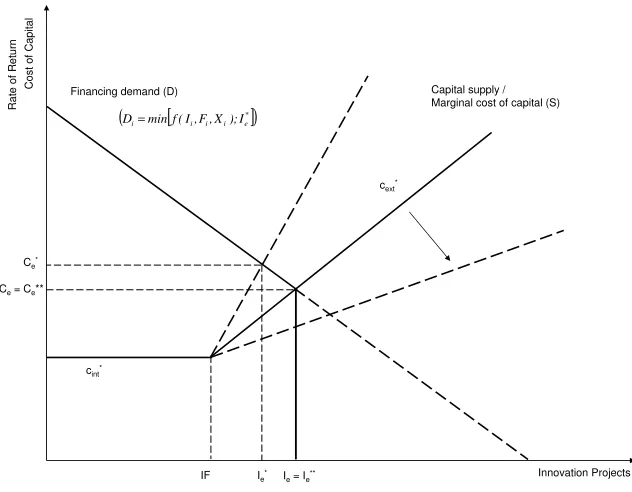
Figure 1.1 provides the standard model, which hereafter is referred to as “long
run equilibrium model”. Di is the capital demand curve of the firm,
repre-senting the marginal revenues of capital depending on the level of innovative
3The model inter alia is used by Howe and Mc Fetridge (1976), Carpenter and Petersen
output. The marginal revenues of capital depend on the level of innovation
expenditures Ii, firm-specific characteristics Fi and industry characteristics
Xi. The capital demand curve therefore is defined as Di =f(Ii, Fi, Xi). Si
is the capital supply curve for the company, representing the marginal costs of capital depending on the level of innovative output. As there exist two sources of capital supply – internal as well as external sources – we assume a pecking order. This means that in the first place the firms will use their
inter-nal funds IFi. Afterwards they will start to obtain external financing, with
a positive relationship between the amount of capital and marginal costs. The intersection of the supply and the demand curves constitutes the
equi-librium innovative outputIe. In this setting, worsening financing conditions,
represented by a steeper supply curve, will lead to higher marginal costs in equilibrium and lower innovative output. Vice versa, improving financing conditions, represented by a flatter supply curve, will lead to lower marginal costs in equilibrium and higher innovative output.
Figure 1.1: Conceptual Framework – Long Run Equilibrium
cext*
R
a
te
o
f
R
e
tu
rn
Innovation Projects
C
o
s
t
o
f
C
a
p
it
a
l
Financing demand (D) Capital supply / Marginal cost of capital (S)
Ie
ce
Ie**
cint*
IF Ce**
Ce*
Ie*
To underpin our novel findings at the empirical level – the existence of asym-metries in the effects of above average and below average financing conditions – we now distinguish between the long run equilibrium provided above and a short run equilibrium derived in the following. By this means we introduce the concept of innovation capacity and short term rigidities with respect to the adjustment of the level of input factors to R&D. The individual innova-tion capacity is defined as the number of potential innovainnova-tion projects the firm is able to produce over a certain period. It may be determined by the amount of different input factors to R&D – such as the number of researchers allocated to R&D, their level of know-how or the quality of the technical equipment related to R&D. How much of these input factors a company ac-cumulates depends on the firm’s individual capital costs and is determined in the long run equilibrium (see Figure 1.1). In the long run the firm will choose its level of input factors to R&D – and accordingly its innovation
ca-pacity – such that it can produce exactly Ie of potential innovation projects.
If it produces on average less than Ie potential projects, this is inefficient as
additional innovation projects still will yield positive net marginal revenues
but cannot be undertaken. If it produces on average more than Ie potential
projects, it is inefficient as not all of the available innovation projects can be undertaken due to negative net marginal revenues.
However, by introducing adjustment rigidities with respect to the input fac-tors to R&D, the implications of the model differ from before. Specifically – and in contrast to the long run equilibrium model – the firms now are facing
a demand function of Di =min[f(Ii, Fi, Xi]);Ie∗]. This means that the
de-mand curve now is kinked at point Ie (see Figure 1.2). By this we take into
account that – due to the presence of the adjustment rigidities introduced in the model – in the short run the innovative output cannot be increased above its maximum level (which is determined by the firm’s innovative
capac-ity, its long run equilibriumIe). As one can see, in this framework worsening
financing conditions, represented by a steeper supply curve, again lead to less potential innovation projects being undertaken. However, unlike in the long run equilibrium model, improving financing conditions, represented by a flatter supply curve, now have no positive effect on the level of innovative output, as the maximum level of potential innovative projects is limited to Ie.
dete-rioration of financing conditions decreases innovative activity, while an im-provement will not foster it (in the short run).
Figure 1.2: Conceptual Framework – Short Run Equilibrium
R
a
te
o
f
R
e
tu
rn
Innovation Projects
C
o
s
t
o
f
C
a
p
it
a
l
Financing demand (D)
cint*
IF Ce*
Ie* Ie= Ie**
Ce= Ce**
[ ]
( *)
e i i i i minf(I,F,X );I
D=
cext*
Capital supply / Marginal cost of capital (S)
1.3
Data
To perform our analysis we use data from two sources: the Ifo Innovation
Sur-vey and the Ifo Business Tendency SurSur-vey for German manufacturing firms.4
As the surveys include questions which are asked on different frequencies, we will transform all variables that are used to the lowest frequency (annual) if necessary.
The Ifo Innovation Survey is carried out annually. The survey inter alia
4Both datasets are provided by the Economics & Business Data Center (EBDC), a
asks the firms,5 if they have “started or continued” an innovation project in the preceding year. As the survey additionally provides information as to whether the company has “finished” or “stopped” an innovation project, we can correct for years in which the company only continued an
innova-tion project.6 Innovations are categorized as either product or process
in-novations. The resulting variables are the variable “productinnov”, which is
coded 1, if a product innovation has started in the corresponding year, and
0 otherwise, and the variable “processinnov”, which is coded 1, if a process
innovation has started in the corresponding year, and 0 otherwise.
The Ifo Business Tendency Survey is carried out monthly and contains ques-tions asked at different frequencies. One of the quesques-tions regards the financ-ing conditions the firms are facfinanc-ing and is included in the survey biannually. The answers are coded as -1 (“favourable financing conditions”), 0 (“nor-mal financing conditions”), and +1 (“reserved financing conditions”). These data are aggregated on an annual basis by taking the averages of the values
of the variable for each year. The variable “credit” resulting from this can
be interpreted as the average financing conditions over the year. It can take values of 1, 0.5, 0, -0.5, or -1, where the limit value of 1 implies that the company reported below average financing conditions at both inquiry dates of the year, and the limit value of -1 implies that the company reported above
average financing conditions at both inquiry dates of the year.7
5Note that each ID-number of the dataset is representing a single production entity for
a single product of the firm rather than the whole firm. This aspect is a further advantage of the dataset as it allows a more detailed analysis for multi-product firms. However, for simplicity, in the following we will refer to the particular unit of observation as “firm”.
6To correct the original variable for values indicating only a continuation of an
innova-tion project we proceed as follows. The value of the variable at time t will be converted from 1 to 0 (i.e. the value of 1 of the variable is indicating a continuation rather than the start of an innovation project), if there was a start or continuation of an innovation project in the preceding year (and no finish or stop of an innovation project), and concurrently no finish or stop of an innovation project in the current period (to prevent that a new innovation project was started after finishing or stopping another process within the same year). The possibility that there exist multiple product or process innovations at the same time is mostly prevented by the fact that each ID-number of the dataset represents a single production entity for a single product of the firm rather than the whole firm. However, the estimations using the dataset without the correction provide qualitatively the same results (see Appendix C).
7Furthermore, a value of 0.5 indicates that the corresponding firm reported below
Furthermore, the Ifo business tendency service consists of questions on the
overall business situation of the firm (“situat”) and on the overall
expec-tations of the firm (“expect”)8. The answers to the question regarding the
business situation of the firm are coded as -1 (“bad business situation”), 0 (“normal business situation”), and +1 (“good business situation”). The answers to the question regarding the firms’ expectations are coded as -1 (“expectations worsened”), 0 (“expectations remained constant”), and +1 (“expectations increased”). As the questions on the business situation and the expectations of the companies are conducted monthly, the corresponding variables also have to be aggregated on an annual basis. We do this by again taking the averages of the values of the variables for each year. The variables resulting from this can be interpreted as the average business situation over the year and the change in the firm’s expectations over the year, respectively.
Finally, the business tendency survey provides information on certain firm characteristics. First of all we can relate to the size of a company in terms of
its market power (“mkp”), which is defined as the number of employees per
firm divided by the number of employees in the firm’s branch. In addition, each firm is allocated to one of the following 14 manufacturing subsectors: Food, Beverages and Tobacco; Textiles and Textile Products; Tanning and Dressing of Leather; Cork and Wood Products except Furniture; Pulp, Pa-per, Publishing and Printing; Refined Petroleum Products; Chemicals and Chemical Products; Rubber and Plastic Products; Other Non-metallic Min-eral Products; Basic and Fabricated Metal Products; Machinery and Equip-ment; Electrical and Optical EquipEquip-ment; Transport EquipEquip-ment; Furniture, Manufacture. Furthermore, each firm is allocated to one of the following regions in Germany: East Germany, West Germany, South Germany and North Germany.
at the other inquiry date of the year. Correspondingly, a value of -0.5 indicates that the corresponding firm reported above average financing conditions at one inquiry date of the year and normal financing condition at the other inquiry date of the year. When the vari-able takes the value 0, the companies mostly have reported normal financing conditions at both inqiry dates. The situation that a company has reported above average financing conditions at one inquiry date of the year and below average financing conditions at the other inquiry date of the year, which also results in a value of the variable of 0, accounts only for a small minority of cases (34 out of 2898 cases, representing 1.17% of the whole sample).
8The variable refers to the expectations the firms are facing with respect to the following
We use data for the period from 2003 to 2007. The dataset is organized as an unbalanced panel. The total number of observations is about 3,000. A more detailed overview about the questionnaire and the survey variables can be found in Becker and Wohlrabe (2008).
1.4
The Model
1.4.1
Specification
To identify possible effects of credit restrictions on the innovative activity of firms we specify the model as
yit =αit+β1creditit+β2expectit+β3situatit+β4mkpit+
+β5exitit+β6Bit+β7Lit+β8Tit+uit.
In our first specification, yit is a dummy variable with value 1, if firm i
started an innovation project (product or process innovation) at time t, and
0 otherwise. In our second and third specifications we distinguish between product and process innovations. Specifically, we estimate a second model
in which yit is a dummy variable with value 1, if firm i started a product
innovation project at time t, and 0 otherwise. Similarly, we estimate a third
model in which yit is a dummy variable with value 1, if firm i started a
process innovation project at time t, and 0 otherwise.
The variable “credit” represents the financing conditions the firm is facing.
The higher the value of the variable, the worse the financing conditions over the year. It is worthwhile to note that the innovation question in the survey refers to the start of an innovation activity rather than the achievement of an innovation. From this follows that the variable is included contemporane-ously, as it is highly likely that the timing of the financing of an innovation project is assigned closely to the actual beginning of an innovation activity. To identify any asymmetries in the effects of below average and above aver-age financing conditions, we provide alternative specifications where we split
the variable “credit” into two dummy variables. In particular, we create one
dummy variable which is coded 1, if the financing conditions over the year
a second dummy variable which is coded 1, if the financing conditions over
the year were better than normal, and 0 otherwise (“crediteas”).
Furthermore, the firms’ decisions to start an innovation project very likely are influenced by their expectations. As our dataset includes information about the firms’ expectations, we have the almost unique possibility to control for
this aspect. Consequently, the variable “expect” is introduced, representing
the change in expectations of the firm over the year. The higher the value of the variable, the more the expectations of the company improved over the
year. As the variable “credit”, the variable “expect” is included
contempo-raneously as a firm will take into account the current rather than the past expectations when deciding to start an innovation project. To capture the ef-fects of firm-specific developments we control for the actual business situation of the firm. The business situation of the firm is represented by the variable
“situat”, which is the higher the better the business situation was over the
year. Similarly to the variable“expect”, the variable“situat”is included
con-temporaneously as a firm will take into account current rather than past firm developments when deciding to start an innovation project. Beside this, we
introduce the variable“mkp”, which represents the size of the firm in terms of
its relative number of employees compared to the competitors of its branch. This variable might be of potential relevance as previous research provides evidence for a clearly positive relationship between the market power and the level of innovative activity of a firm.
In addition, we control for certain other firm characteristics. To account for a heterogeneous level of innovation activity between firms of different branches
we include vector Bit, a set of 13 dummy variables which indicate the
affil-iation of the firm to a specific branch.9 For similar reasons – heterogeneity
in the innovation activity of companies of different regions – we include a
further set of dummy variables, represented by vector Lit, which consists of 3
dummy variables indicating the region the company is allocated to.10
More-over, to take into account possible changes of the innovative behaviour over time due to major technological or structural developments, we introduce
vector Tit, which consists of 4 time dummies representing the years 2004 to
2007.11
9The baseline branch is the branch “Machinery and Equipment”.
10The baseline region is North Germany.
Finally, we have to address a possible sample selection bias due to attrition,12 as some companies initially included in the survey were discharged from the survey over time. The main reasons for discharging usually are that the com-pany is no longer interested in taking part in the survey, that the comcom-pany was taken over by another firm or that the company went bankrupt. If the exit of the companies is not random and there exist some common underlying reasons that the companies left the survey – e.g. bad overall performance – there could be some source of sample selection bias in our estimations. In
order to ease this problem we include the dummy variable “exit”, which
in-dicates if a firm has left the survey over the period of the analysis, thereby capturing firm-specific common characteristics of those firms which were dis-charged from the survey (see Smolny, 1996).
1.4.2
The Aspect of Endogeneity
As in most analyses, one major point to address is that of endogeneity in its various forms. This short section deals with this aspect. Specifically, it lists the different potentially relevant types of endogeneity, discusses how they are related to our analysis and how the analysis deals with these different types, if necessary.
The first source of endogeneity is unobserved heterogeneity. In this context one has to note that the design of the questions of interest in the survey is
such that by their nature firm fixed effects are eliminated.13 This leaves α
it,
representing the firm-specific effects, and our independent variables uncorre-lated and leads us in a first regression to the use of a random effects model, thereby avoiding the incidental parameter problem commonly present when applying a fixed effects estimator in this setting (Neyman and Scott, 1948,
Hausman et al., 1984).14
12See Heckman (1979), Smolny (1998).
13The survey asks for the financing conditions and the business situation compared to
their normal firm-specific levels (normal, better than normal, worse than normal), which by definition eliminates the firm fixed effects with respect to these variables (similarly to a within-transformation). Furthermore, the survey asks for the change in business expec-tations on an ordinal scale (improvement/deterioration/no change of business situation), which also rules out any firm fixed effects concerning this variable.
14The use of the random effects estimator is also supported by the results of a Hausman
The second source of endogeneity possibly relevant is simultaneity between the response variable and our explanatory variables. For example, it might not only be possible that a firm’s decision to innovate is influenced by the firm-specific financing conditions, but also that the firm-specific financing conditions are influenced by the firm’s decision to innovate. We can control for this by again using the panel structure of our dataset. In particular, we apply a two stage least squares instrumental variable probit estimator, which allows to instrument our potentially endogenous explaining variables by their first lags.
Finally, when estimating our models for the start of process and product innovations separately, we have to consider the possible simultaneity of these two decisions. Specifically, there exists the possibility that the decision of starting a product innovation is made conditional on the decision of starting a process innovation and vice versa. To take into account this potential dependency we additionally apply a bivariate probit estimator when dealing with these variables.
1.5
Results
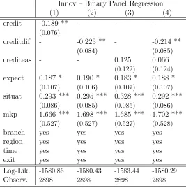
Table 1.1 provides the results of our random effects probit panel estimator. It shows how the financing conditions the firms are facing relate to the prob-ability of the start of an innovation project (product or process innovation project) in the corresponding year.
First, when including our original measure of the credit situation in Specifica-tion 1 we can observe a clearly significant and negative relaSpecifica-tionship between worsening financing conditions and the probability that a firm will start an innovation project. The worse the financing conditions (the higher the value
of our variable “credit”), the smaller the probability that the firm will start
an innovation project in the corresponding year (see Column 1).
Secondly, when splitting our financing conditions measure into below average
(“creditdif ”) and above average (“crediteas”) financing conditions and
ing our original variable on the financing conditions with these new variables, we can observe some asymmetries. The results, presented in Columns 2-4 of Table 1.1, show that financing conditions which were worse than normal
(“creditdif ”=1) indeed decrease the probability that a firm will start an
in-novation project, but that in contrast – and against the standard theory –
financing conditions which were better than normal (“crediteas”=1)
appar-ently do not have a significantly positive effect.
Table 1.1: Credit Constraints and Innovative Activity – Random Effects Probit Model
Innov – Binary Panel Regression
(1) (2) (3) (4)
credit -0.189 ** - -
-(0.076)
creditdif - -0.223 ** - -0.214 **
(0.084) (0.085)
crediteas - - 0.125 0.066
(0.122) (0.124)
expect 0.187 * 0.190 * 0.183 * 0.188 *
(0.107) (0.106) (0.107) (0.107)
situat 0.293 *** 0.295 *** 0.328 *** 0.292 ***
(0.086) (0.085) (0.085) (0.086)
mkp 1.666 *** 1.698 *** 1.685 *** 1.702 ***
(0.527) (0.527) (0.527) (0.528)
branch yes yes yes yes
region yes yes yes yes
time yes yes yes yes
exit yes yes yes yes
Log-Lik. -1580.86 -1580.43 -1583.44 -1580.29
Observ. 2898 2898 2898 2898
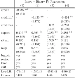
As discussed in Section 4, there might exist some potential endogeneity bias due to simultaneity between the dependent variable and its regressors. To prove that our results are not driven by this aspect we perform an instru-mental variable estimation, in which we tackle this issue. Specifically, we apply a two stage least squares probit instrumental variable estimator as an additional robustness check. Consequently, our potential endogenous vari-ables – the varivari-ables on the financing conditions, the variable on the state of the business and the variable on the change in the expectations of the firm – are instrumented by their first lags. For all these instruments the first stage
regressions indicate that they are significant and strong instruments.15
The results of the second stage regressions are presented in Table 1.2. In Column 1 we again can observe a clearly negative and significant effect of worsening financing conditions on the innovative activity of firms, which is in line with our previous findings. Furthermore, also the results of the es-timations when including the two separate variables for above average and below average financing conditions, presented in Columns 2-4, support and even strengthen the findings of our preceding estimations. As before we find that below average financing conditions restrict innovative activity, whereas above average financing conditions do not foster it. In this context it is worthwhile to note that the coefficients of the IV-estimator for our variables “credit” and “creditdiff” are higher than in our baseline estimations, sug-gesting an underestimation of the effects of worsening financing conditions on the innovative activity of firms when not taking into account the aspect of mutual causation. By this, our results support findings of previous literature highlighting the reverse causality between credit restrictions and innovative activity (Hajivassiliou and Savignac, 2007, Savignac, 2008).
Table 1.2: Credit Constraints and Innovative Activity – Instrumental Variable Probit Model
Innov – Binary IV Regression
(1) (2) (3) (4)
credit -0.297 ** - -
-(0.134)
creditdif - -0.430 ** - -0.494 **
(0.174) (0.213)
crediteas - - 0.002 -0.233
(0.384) (0.438)
expect 0.416 ** 0.393 ** 0.385 ** 0.389 **
(0.345) (0.166) (0.165) (0.166)
situat 0.485 0.157 0.309 ** 0.171
(0.271) (0.134) (0.130) (0.136)
mkp 1.094 0.875 0.778 0.865
(0.848) (0.588) (0.580) (0.590)
branch yes yes yes yes
region yes yes yes yes
time yes yes yes yes
exit yes yes yes yes
Log-Lik. -764.19 -1580.43 -1583.44 -1580.29
Observ. 1489 1489 1489 1489
***: p <0.01; **: p <0.05; *: p <0.1. Standard errors in parentheses.
A further feature of our dataset is the possibility to distinguish between prod-uct and process innovations. This allows to apply some additional robustness checks by performing our analysis for the two kinds of innovative activity separately. Specifically, we can examine if the previous results hold when distinguishing between process and product innovations. Table 1.3 provides the results of our random effects panel estimator for both kinds of innovative activity. Table 1.4 provides the results of our two stage instrumental variable
estimator.16 As already mentioned in Section 4, when distinguishing between
the decision to start a product innovation and the decision to start a process innovation, we have to consider in addition the possible simultaneity of the
16Again, also here the first stage regressions indicate our instruments are significant and
two decisions. Consequently, in Table 1.5 we provide the results when ap-plying a bivariate probit estimator to account for the potential dependency of the two decisions.
Columns 1-4 of each table provide the results regarding the probability to start a product innovation project, Columns 5-8 of each table provide the results regarding the probability to start a process innovation project. How-ever, one can see that for both kinds of innovative activity the outcomes again support our previous findings. All estimations show a clearly significant and negative relationship between worsening financing conditions and the prob-ability that the firm will start a product or process innovation project, re-spectively. Moreover, the results again show that below average financing conditions have a negative effect on the decisions to start product as well as process innovation projects and that above average financing conditions do not foster them, thereby supporting previous findings and conclusions.
Table 1.3: The Differentiation between Product- and Process Innovations – Random Effects Panel Probit Model
Productinnov – Binary Panel Regression Processinnov – Binary Panel Regression
(1) (2) (3) (4) (5) (6) (7) (8)
credit -0.229 *** - - - -0.190 ** - -
-(0.076) (0.075)
creditdif - -0.244 *** - -0.233 *** - -0.187 ** - -0.165 *
(0.084) (0.085) (0.083) (0.085)
crediteas - - 0.145 0.080 - - 0.213 * 0.166
(0.122) (0.123) (0.121) (0.122)
expect 0.193 ** 0.200 ** 0.235 *** 0.196 ** 0.298 *** 0.306 *** 0.328 *** 0.299 ***
(0.085) (0.084) (0.084) (0.085) (0.084) (0.084) (0.083) (0.084)
situat 0.272 ** 0.275 ** 0.265 ** 0.273 ** 0.033 0.036 0.028 0.031
(0.107) (0.107) (0.108) (0.107) (0.105) (0.105) (0.105) (0.105)
mkp 0.907 * 0.939 * 0.939 * 0.944 * 1.136 ** 1.159 ** 1.172 ** 1.171 **
(0.484) (0.483) (0.486) (0.483) (0.459) (0.459) (0.461) (0.460)
branch yes yes yes yes yes yes yes yes
region yes yes yes yes yes yes yes yes
time yes yes yes yes yes yes yes yes
exit yes yes yes yes yes yes yes yes
Log-Lik. -1501.75 -1502.08 -1501.87 -1505.58 -1376.95 -1377.63 -1378.58 -1376.71
Observ. 2898 2898 2898 2898 2898 2898 2898 2898
Table 1.4: The Differentiation between Product- and Process Innovations – Instrumental Variable Probit Model
Productinnov – Binary IV Regression Processinnov – Binary IV Regression (1) (2) (3) (4) (5) (6) (7) (8) credit -0.301 ** - - - -0.425 *** - -
-(0.146) (0.157)
creditdif - -0.457 ** - -0.448 ** - -0.591 *** - -0.669 ***
(0.177) (0.217) (0.190) (0.234)
crediteas - - 0.245 0.033 - - 0.032 -0.283
(0.386) (0.439) (0.422) (0.485)
expect 0.155 0.124 0.248 * 0.122 0.162 0.141 0.341 ** 0.155
(0.136) (0.136) (0.132) (0.139) (0.145) (0.146) (0.141) (0.148)
situat 0.297 ** 0.291 * 0.288 * 0.291 * 0.338 0.329 * 0.317 * 0.325 *
(0.168) (0.169) (0.168) (0.169) (0.180) (0.181) (0.179) (0.182)
mkp -0.156 -0.102 -0.151 -0.100 1.062 * 1.140 * 0.999 ** 1.136 *
(0.654) (0.658) (0.647) (0.659) (0.591) (0.596) (0.585) (0.600)
branch yes yes yes yes yes yes yes yes region yes yes yes yes yes yes yes yes time yes yes yes yes yes yes yes yes exit yes yes yes yes yes yes yes yes Observ. 1489 1489 1489 1489 1489 1489 1489 1489 ***:p <0.01; **:p <0.05; *:p <0.1. Standard errors in parentheses.
Table 1.5: The Differentiation between Product- and Process Innovations – Binary Bivariate Probit Model
Productinnov – Binary Bivariate Regression Procesinnov – Binary Bivariate Regression
(1a) (2a) (3a) (4a) (1b) (2b) (3b) (4b)
credit -0.202 *** - - - -0.190 *** - -
-(0.051) (0.053)
creditdif - -0.234 *** - -0.231 *** - -0.222 *** - -0.215 ***
(0.057) (0.058) (0.059) (0.060)
crediteas - - 0.092 0.021 - - 0.114 0.049
(0.085) (0.087) (0.086) (0.088)
expect 0.149 *** 0.153 *** 0.196 *** 0.151 *** 0.236 *** 0.240 *** 0.278 *** 0.236 ***
(0.054) (0.054) (0.053) (0.054) (0.057) (0.056) (0.056) (0.057)
situat 0.228 *** 0.229 *** 0.224 *** 0.229 *** 0.081 0.081 0.078 0.081
(0.069) (0.069) (0.068) (0.069) (0.072) (0.072) (0.072) (0.072)
mkp 0.740 ** 0.763 ** 0.763 ** 0.765 ** 0.826 *** 0.846 *** 0.849 *** 0.850 ***
(0.326) (0.329) (0.323) (0.329) (0.315) (0.312) (0.317) (0.312)
branch yes yes yes yes yes yes yes yes
region yes yes yes yes yes yes yes yes
time yes yes yes yes yes yes yes yes
exit yes yes yes yes yes yes yes yes
Log-Lik. -2760.19 -2759.13 -2768.59 -2758.98 -2760.19 -2759.13 -2768.59 -2758.98
Observ. 2898 2898 2898 2898 2898 2898 2898 2898
1.6
Summary and Conclusion
In this essay we have analysed the effects of financing conditions on the in-novative activity of firms. In contrast to other literature we could use direct measures for the innovative activity of the firms as well as for the financing conditions the firms are facing, by this means avoiding problems of indirect measures commonly applied as proxies for these two variables. Moreover, the dataset provided the possibility to control for the business expectations of a firm – due to the existence of forward-looking adjustments in a world of expectations an important determinant of the innovative activity of the firm. In addition, the characteristics of the dataset and the design of the sur-vey questions allowed us to avoid endogeneity issues caused by unobserved heterogeneity or mutual causation, which commonly are present in the liter-ature. Finally, the possibility to differentiate between ”worse than average” and “better than average” financing conditions allowed us to analyse poten-tial asymmetries in the effects of below average and above average financing conditions.
The results provided – as opposed to many other papers – strong evidence that worsening financing conditions restrict the innovative activity of firms. More interestingly, the results showed asymmetries in the effects of below average and above average financing conditions. We found that below aver-age financing conditions restrict innovative activity, whereas above averaver-age financing conditions do not foster it. The novel second result on the exis-tence of asymmetries has interesting implications. It gives strong evidence for considerations raised in more recent literature that the individual inno-vation capacity of a firm plays an important role for its innovative activity. To additionally support our findings we have extended the usual theory of innovation activity by rigidities with respect to a firm’s individual innovation capacity, which leads to a differentiation between a long run and a short run equilibrium in innovative output.
Acknowledgements
References
Alti, A., (2003), “How Sensitive is Investment to Cash Flow when Financing is Frictionless?”, The Journal of Finance 58(2), pp. 707-722.
Atzeni, G. and Piga, C., (2007), “R&D Investment, Credit Rationing and Sample Selection”, Bulletin of Economic Research 59(2), pp. 149-178.
Becker, S. O. and Wohlrabe, K., (2008), “Micro Data at the Ifo Institute for Economic Research – The “Ifo Business Survey”, Usage and Access”, Journal of Applied Social Science Studies 128(2), pp. 307-319.
Bhagat, S. and Welch, I., (1995), “Corporate Research & Development In-vestments International Comparisons”, Journal of Accounting and Eco-nomics 19, pp. 443-470.
Binz, H. L. and Czarnitzki, D., (2008), “Financial Constraints: Routine versus Cutting Edge R&D Investment”, Journal of Economics and Man-agement Strategy, forthcoming.
Bond, S., Harhoff, D. and Van Reenen, J., (2006), “Investment, R&D and Financial Constraints in Britain and Germany”, Annales d’conomie et de Statistique, forthcoming.
Carpenter, R. E. and Petersen, B. C., (2002), “Is the Growth of Small Firms Constrained by Internal Finance?”, The Review of Economics and Statis-tics 84(2), pp. 298-309.
Hajivassiliou, V. and Savignac, F., (2007), “Financing Constraints and a Firm’s Decision and Ability to Innovate: Establishing Direct and Reverse Effects.”, FMG Discussion Paper 594.
Hall, B. H., Mairesse, J. and Mulkay, B., (2001), “Firm Level Investment and R&D in France and in the United States”, Deutsche Bundesbank (ed), Investing Today for the World of Tomorrow, Springer Verlag.
Harhoff, D., (1998), “Are there Financing Constraints for R&D and Invest-ment in German Manufacturing Firms?”, Annales d’Economie et de Statis-tique 49/50, pp. 421-456.
for Count Data with an Application to the Patents - R&D Relationship”, Econometrica 52(4), pp. 909-938.
Heckman, J.J., (1979), “Sample Selection Bias as a Specification Error”, Econometrica, 47(1), pp. 153-61.
Hottenrott, H. and Peters, B., (2009), “Innovative Capability and Financing Constraints for Innovation More Money, More Innovation?”, ZEW Discus-sion Paper No. 09-081.
Howe, J. D. and Mc Fetridge, D. G., (1976), “The Determinants of R&D Expenditures”, Canadian Journal of Economics 9, pp. 57-71.
Kaplan, S. and Zingales, L., (1997). “Do Investment-Cash Flow Sensitivities Provide Useful Measures of Financing Constraints?”, Quarterly Journal of Economics 112, pp. 169-215.
Neyman, J. and Scott, E. L., (1948), “Consistent Estimation from Partially Consistent Observations”, Econometrica 16, pp. 1-32.
Savignac, F., (2006), “The Impact of Financial Constraints on Innovation: Evidence from French Manufacturing Firms”, Cahiers de la Maison des Sciences Economiques, Universit Panthon-Sorbonne (Paris 1).
Savignac F., (2008), “Impact of Financial Constraints on Innovation: What Can Be Learned from a Direct Measure?”, Economics of Innovation and New Technology, 17(6), pp. 553-569.
Smolny, W., (1996), “Innovation, Prices, and Employment – a Theoreti-cal Model and an EmpiriTheoreti-cal Application for West German Manufacturing Firms”, Center for International Labor Economics, University of Konstanz, Discussion Paper, 37.
Appendix
A Results of the Hausman Test
Table 1.6: Hausman Test – Baseline Specification with Dependent Variable “Innov”
(b) (B) (b-B) (sqrt(diag(Vb−VB)))
(fixed effects) (random effects) (difference) (s.e.)
credit -0.019 -0.043 0.024 0.018
expect -0.006 0.040 -0.046 0.029
situat 0.058 0.066 -0.008 0.023
d 2004 -0.033 -0.030 -0.002 0.014
d 2005 -0.033 -0.021 -0.012 0.015
d 2006 -0.025 -0.036 0.011 0.018
d 2007 -0.030 -0.047 0.017 0.021
b = consistent under H0 and Ha; obtained from linear fixed effects panel estimator. B = inconsistent under Ha, efficient under H0; obtained from linear random effects panel estimator.
Test: H0: difference in coefficients not systematic
χ2(8) = (b−B)0[(Vb−VB)(−1)](b−B) = 6.44
P rob > χ2= 0.5978
Table 1.7: Hausman Test – Baseline Specification with Dependent Variable “Productinnov”
(b) (B) (b-B) (sqrt(diag(Vb−VB)))
(fixed effects) (random effects) (difference) (s.e.)
credit -0.023 -0.049 0.025 0.019
expect 0.010 0.054 -0.043 0.027
situat 0.027 0.041 -0.014 0.025
d 2004 -0.009 -0.010 0.001 0.013
d 2005 -0.002 -0.005 0.003 0.014
d 2006 -0.008 -0.025 0.017 0.018
d 2007 -0.014 -0.036 0.022 0.020
b = consistent under H0 and Ha; obtained from linear fixed effects panel estimator. B = inconsistent under Ha, efficient under H0; obtained from linear random effects panel estimator.
Test: H0: difference in coefficients not systematic
χ2(8) = (b−B)0[(Vb−VB)(−1)](b−B) = 7.05
Table 1.8: Hausman Test – Baseline Specification with Dependent Variable “Processinnov”
(b) (B) (b-B) (sqrt(diag(Vb−VB)))
(fixed effects) (random effects) (difference) (s.e.)
credit 0.009 -0.039 0.048 0.018
expect -0.026 0.004 -0.030 0.030
situat 0.040 0.058 -0.019 0.023
d 2004 -0.042 -0.045 0.003 0.012
d 2005 -0.043 -0.032 -0.011 0.014
d 2006 -0.030 -0.046 0.016 0.018
d 2007 -0.038 -0.068 0.030 0.017
b = consistent under H0 and Ha; obtained from linear fixed effects panel estimator. B = inconsistent under Ha, efficient under H0; obtained from linear random effects panel estimator.
Test: H0: difference in coefficients not systematic
χ2(8) = (b−B)0[(V
b−VB)(−1)](b−B) = 12.40
B Robustness Check – First Lag of Dependent
Variable as Additional Regressor
Table 1.9: Robustness Check – Lag of Dependent Variable Included as Additional Regressor
Innov Productinnov Processinnov (1) (2) (3) (4) (5) (6) credit -0.185 ** -0.202 ** - -0.212 **
-(0.086) (0.090) (0.106)
creditdif - -0.234 ** - -0.240 ** - -0.200 *
(0.095) (0.099) (0.117)
crediteas - 0.025 - 0.013 - 0.168
(0.140) (0.144) (0.164)
expect 0.154 0.153 0.189 0.188 0.120 0.115
(0.116) (0.116) (0.122) (0.122) (0.145) (0.145)
situat 0.349 *** 0.345 *** 0.251 ** 0.251 ** 0.484 *** 0.481 ***
(0.095) (0.095) (0.097) (0.097) (0.119) (0.119)
mkp 1.539 *** 1.569 *** 0.925 * 0.963 * 0.820 0.851
(0.589) (0.589) (0.576) (0.574) (0.692) (0.692)
branch yes yes yes yes yes yes region yes yes yes yes yes yes time yes yes yes yes yes yes exit yes yes yes yes yes yes Log-Lik. -1013.20 -1012.28 -971.63 -971.09 -860.25 -859.92
Observ. 1999 1999 1999 1999 1999 1999 Random effects probit model. + First lag of the dependent variable.
C Robustness Check – Dataset without
Cor-rections
Table 1.10: Robustness Check – Use of the Initial Dataset without Corrections
Innov Productinnov Processinnov (1) (2) (3) (4) (5) (6) credit -0.199 ** - -0.236 *** - -0.188 **
-(0.084) (0.085) (0.083)
creditdif - -0.199 ** - -0.221 ** - -0.160 *
(0.095) (0.095) (0.094)
crediteas - 0.119 - 0.165 - 0.189
(0.138) (0.137) (0.136)
expect 0.295 ** 0.294 ** 0.360 *** 0.360 *** 0.045 0.042
(0.120) (0.120) (0.122) (0.122) (0.118) (0.118)
situat 0.254 *** 0.253 *** 0.155 0.155 0.386 0.388
(0.096) (0.096) (0.096) (0.096) (0.095) *** (0.095) ***
mkp -0.338 -0.322 -0.213 -0.197 0.038 0.053
(0.614) (0.613) (0.598) (0.597) (0.585) (0.584)
branch yes yes yes yes yes yes region yes yes yes yes yes yes time yes yes yes yes yes yes exit yes yes yes yes yes yes Log-Lik. -1544.69 -1544.46 -1481.58 -1481.36 -1396.41 -1395.99
Observ. 2898 2898 2898 2898 2898 2898
Random effects probit model. ***: p < 0.01; **: p <0.05; *: p < 0.1.
Chapter 2
Product and Process
Innovations and Growth – New
Evidence from Firm Level
Panel Data
2.1
Introduction
At the micro level, competitiveness is generally defined as the ability of a company to grow. In earlier literature, mainly price factors – e.g. cost reduc-tions – were considered as determining the competitiveness of a firm. This view was questioned by the publication of Kaldor (1978) along with the so called Kaldor paradox. The Kaldor paradox describes the empirical finding that countries which experience a significant increase in their labour costs often concurrently experience an increase in their export shares. In light of this, by using several measures for the growth of the companies, a huge body of literature appeared, which considered non-price factors – especially in terms of innovations – as important determinants of the competitiveness of firms. In this framework, most prominent and vital branches of research discuss the influence of innovative activity on export shares (see e.g. Ster-lacchini, 1999, Roper and Love, 2002, Bleaney and Wakelin, 2002) or on the level of employment (see e.g. Piva and Vivarelli, 2005, Bogliacino and Pianta, 2010, or Chennels and Van Reenen, 2002, for an overview).
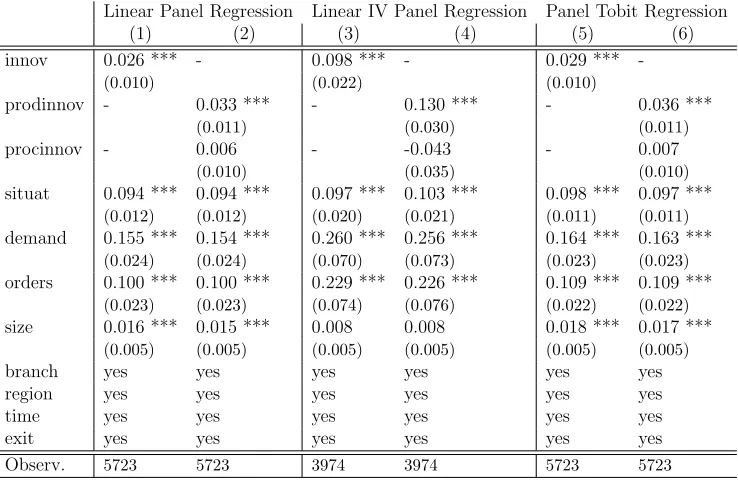
The results highlight the major importance of innovations for growth. By using a direct measure of the competitive situation of a firm as well as for the innovative activity of a firm we find a clearly significant and positive effect of innovative activity – at the national as well as at the international level. More importantly, when distinguishing between product and process innova-tions we find that only the introduction of product innovainnova-tions significantly contributes to an improvement in the competitive situation of the firm, while we cannot observe this for the introduction of process innovations. This re-sult provides evidence that non-price factors indeed play a superior role for competitiveness and growth compared with price factors.
Consequently, the remainder of the essay is organized as follows. Section
2 provides some information about the dataset. Section 3 describes our
empirical specification. Section 4 presents the estimation results. Section 5 concludes.
2.2
The Survey Data
To perform our analysis we use data from two sources: the Ifo Innovation Survey and the Ifo Business Tendency Survey for German manufacturing
firms.1 In these datasets, the unit of observation for multi product firms
represents a single production entity for a single product of the firm rather than the whole firm, thereby enabling a more detailed analysis than usual. However, for the sake of simplicity, in the following we will refer to a unit of observation as a “firm”. As the surveys include questions which are asked on different frequencies, we will transform all variables used to the lowest frequency (annual) if necessary.
2.2.1
Data from the Ifo Innovation Survey
The data on the innovative activity of the firm stem from the Ifo Innovation Survey, which is conducted annually. Specifically, the survey asks at the
be-1Both datasets are provided by the Economics & Business Data Center (EBDC), a
ginning of each year, whether the firm has introduced an innovation in the preceding year. Innovations are categorized in product and process
innova-tions. The resulting variables are the variable “prodinnov”, which is coded
1, if a product innovation was introduced in the preceding year, and 0
other-wise, and the variable “procinnov”, which is coded 1, if a process innovation
was introduced in the preceding year, and 0 otherwise.2
Table 2.1 provides some descriptive statistics, which will be of importance in the following for some robustness checks. The first two rows present the
frequencies of the outcomes of the variables“prodinnov”and“procinnov”
de-scribed above. The last 4 rows present the joint frequencies of the variables
“prodinnov” and “procinnov”. In particular, row 3 provides the frequency
for the situation in which product and process innovations were introduced
contemporarily (“prod- and procinnov”). Row 4 and row 5 provide the
fre-quencies for the situation in which only a product innovation (“prodinnov
only”), and the situation in which only a process innovation (“procinnov
only”) was introduced. Row 6 shows the frequency for the situation in which
no innovation at all was introduced (“noinnov”).
Table 2.1: Descriptive Statistics – Innovation Variables
yes (1) no (0) total Unconditional prodinnov 3131 4266 7397 Frequencies (42.33 %) (57.67 %) (100.00 %)
procinnov 2248 5149 7397
(30.39 %) (69.61 %) (100.00 %)
Conditional prod- and procinnov 1788 5609 7397 (Joint) (24.17 %) (75.83 %) (100.00 %)
Frequencies prodinnov only 1343 6054 7397
(18.16 %) (81.84 %) (100.00 %)
procinnov only 460 6937 7397
(6.22 %) (93.78 %) (100.00 %)
noinnov 3806 3591 7397
(51.45 %) (48.55 %) (100.00 %)
7397
-(100.00 %)
2The possibility that there exist multiple product or process innovations at the same
2.2.2
Data from the Ifo Business Tendency Survey
The data on the competitive situation of the firm stem from the monthly Ifo business tendency service and are included in the survey quarterly. The survey asks about the change in the competitive situation of the firm at the national level as well as at the European level (excluding the domestic market). For the remainder of the essay we will refer to the latter as the ”international level”. The answers are coded as +1 (“competitive situation improved over the last 3 months”), 0 (“competitive situation remained con-stant over the last 3 months”), and -1 (“competitive situation worsened over the last 3 months”). These data are aggregated on a yearly basis by taking the averages of the values of the variables over the year. The variables result-ing from this can be interpreted as measures of the change in the competitive
situation of the firm at the national level over the year (“compet-nat”) and of
the change in the competitive situation of the firm at the international level
over the year (“compet-int”). They can take values between +1 and -1, where
the limit value of +1 indicates that the firm reported an improvement of the competitive situation at the national/international level in every quarter of the year. Correspondingly, the limit value of -1 indicates that the firm re-ported a worsening in the competitive situation at the national/international level in every quarter of the year.
Furthermore, the Ifo business tendency service consists of a question on the overall business situation of the firm. The answers to this question are coded as -1 (“unfavourable business situation”), 0 (“normal business situation”), and +1 (“good business situation”). Similarly to the question on the com-petitive situation of the firm, the question on the business situation of the firm is asked several times during the year (every month). Accordingly, this variable also has to be aggregated on a yearly basis. We do this again by taking the average of the values of the variable of the single months. The
resulting variable “situat” can be interpreted as the average business
over the year (“demand”) and the change in the number of orders of the firm
over the year (“orders”), respectively.
Finally, the business tendency survey provides information on certain firm characteristics. First of all, we can relate to the size of a company in terms of its number of employees. Specifically, this is done by generating the
vari-able “size”, which is the natural logarithm of the number of employees of
the firm. In addition, each firm is allocated to one of the following 14 man-ufacturing subsectors: Food, Beverages and Tobacco; Textiles and Textile Products; Tanning and Dressing of Leather; Cork and Wood Products ex-cept Furniture; Pulp, Paper, Publishing and Printing; Refined Petroleum Products; Chemicals and Chemical Products; Rubber and Plastic Products; Other Non-metallic Mineral Products; Basic and Fabricated Metal Products; Machinery and Equipment; Electrical and Optical Equipment; Transport Equipment; Furniture, Manufacture. Furthermore, each firm is allocated to one of the following regions in Germany: East Germany, West Germany, South Germany and North Germany.
We use data for the period from 1994 to 2007. The dataset is organized as an unbalanced panel, and the total number of observations is about 7400. A detailed overview of the questionnaire and the survey variables can be found in Becker and Wohlrabe (2008).
2.3
Empirical Specification
To analyse the possible effects of innovative activity on the competitive sit-uation of the firms we specify the baseline model as
yit =αit+β1innovit+β2situatit+β3demandit+β4ordersit+
+β5sizeit+β6exitit+β7Bit+β8Lit+β9Tit+uit,
where yit is the variable representing the competitive situation of firm i at
time t.
In a first specification, our explanatory variable of interest is the variable
“innov”. This variable is a dummy variable, which equals 1, if firm i has