Application Layer Protocol for Network Integration of a Smart Grid Residential Load-Shifting Algorithm

Available Online at www.ijcsmc.com

International Journal of Computer Science and Mobile Computing

A Monthly Journal of Computer Science and Information Technology

ISSN 2320–088X

IJCSMC, Vol. 4, Issue. 10, October 2015, pg.219 – 232

RESEARCH ARTICLE

Application Layer Protocol for Network

Integration of a Smart Grid Residential

Load-Shifting Algorithm

Martin Ivanov

, Rozalina Dimova

Department of Telecommunications, Technical University of Varna, Bulgaria

1 _{[email protected];} 2 _{[email protected]}

Abstract— The iterative and distributed nature of the most recent mechanisms for residential load shifting heavily relies on the smart grid IP-based communication networks that enable them. Nonetheless, little work has been carried out on the practicalities of evaluating the communication parameters that heavily influence the performance of such mechanisms. This study builds on our previous work, a distributed residential load-shifting algorithm for efficient renewable energy consumption, and presents a model of an application layer protocol that integrates the algorithm’s functionality. Simulation results for the communication parameters having negative impact on the performance of the algorithm in terms of available iterations are presented.

Keywords— smart grids, IP-based networks, application protocol, demand response, residential load-shifting

I. INTRODUCTION

Future efforts for increasing the energy consumption flexibility will be facilitated by the emerging smart grid communication infrastructures, providing end consumers, operators and energy suppliers the means for advanced information exchange and demand control. Despite the fact that the debates on the most suitable communication technologies are open, it is clear that the IP-based networks are the game-changing factor for enabling the smart grids [1]-[3]. Such adoption of large spectrum of available network technologies leads to new opportunities for development of novel Demand Response (DR) mechanisms aiming at peak power reduction and stimulation for higher renewable energy consumption. With the growing efforts toward development of communication-enabled residential appliances, household energy management has become an important topic and the emerging automatic appliance scheduling is envisioned to greatly aid in reducing peak loads by shifting the energy consumption in time.

However, the distributed and iterative nature of such algorithms strongly relies on the communication networks that enable it. To the best of our knowledge, the evaluation of network-specific parameters, having negative influence on such algorithms is falling behind. In this context, the study presented here builds on our previous work, an appliance scheduling algorithm for efficient renewable energy consumption [11], in order to study the impact of various network-specific parameters on the performance of the algorithm. The algorithm’s functionality is integrated into a model of application layer network protocol aiming at enabling the algorithm’s performance evaluation in large-scale realistic scenarios.

II. COMMUNICATION ARCHITECTURE OVERVIEW AND CONSIDERATIONS

As described in [11], a discrete time model is used, and an arbitrary but finite receding time horizon is assumed - divided into T time slots with each time slot t∈ {1, 2, …, T} having the same duration td. In each t the

price of electricity can differ due to changes in global consumption and renewable energy generation. The prices are based on generation forecasts and are broadcasted to the consumers in the form of a price vector f = [f1,

f2, … , fT]. Additional energy storage units may be deployed to minimize the losses from forecasting errors due

to prediction uncertainties. Nonetheless, it is assumed that the forecasts are accurate and the mismatch losses are negligible due to the recent advancements in wind and solar generation forecasting methods [12]-[15]. After acquiring pricing data, consumers respond with sending their energy consumption schedules Ek = [Ek1, Ek2,…,

EkT], allowing a centralized logic to analyze the scheduled collective consumption profile and react by

attempting to limit the global consumption in certain t, if the consumption exceeds a predefined renewable generation level and/or peak loads are expected. The choice for T relies mainly on the acceptable accuracy of renewable energy generation forecast time windows, while choosing an appropriate td is based on a large

number of network (packet delays and variations; packet loss and retransmissions) and computational (required time periods for generating energy schedules, pricing and consumption limitation information) parameters.

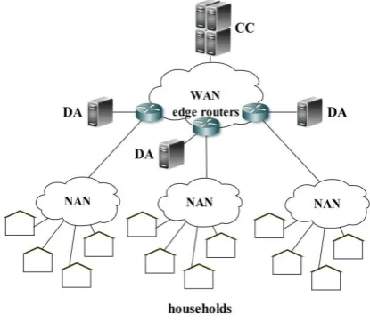
We consider a communication system that consists of multiple households, a central controller (located in a control center) and multiple data aggregators. Households (HHs) are flexible energy consumers, willing to alter their consumption patterns to some extent, in order to reduce their electricity bills. To participate, a HH must be equipped with at least one appliance whose load can be shifted in time (e.g. water heater, clothes dryer, electric vehicle, etc.). The shiftable appliances are networked together via home area network (HAN) and must possess the functionality to respond to control commands concerning their operational behaviour. The households must be also equipped with a home energy management system (EMS). It enables automatic response to changes in the energy prices by storing the household residents’ preferences for appliance operation deadlines and appliance priorities, solving the optimization problem defined in [11], and executing the resulting consumption schedules by controlling the operation of the shiftable appliances. The EMS uses the smart meter’s communication interface as a gateway for exchanging messages, however, smart metering applications are outside the scope of this paper.

The central controller (CC) is deployed in the utility’s server infrastructure and its main goal is to match the renewable energy supply forecasts with the households demand by changing dynamically the energy price and attempting to limit the total energy consumption of the households for a certain t without interfering with the consumers’ preferences.

Fig. 1 System architecture overview

Such a hierarchical architecture is enhancing the topology scalability by allowing cascade connections of multiple DAs. To enable the protocol’s functionality, the communication network must consist minimally of two end communication entities – one CC and at least one household. The existence of a DA is not mandatory as the protocol allow direct interactions between HHs and the CC. However, scenarios without the use of DAs are highly unrealistic and inefficient due to the significant increase in WAN bandwidth requirements and computational requirements in the CC’s infrastructure.

The communication environment in which the protocol is executed is a non-reliable packet-switched medium, hence a reliable communication service must be used, ensuring the lossless data delivery. The Transmission Control Protocol (TCP) is chosen as underlying protocol at the transport layer. Despite the fact that TCP is heavier and more complex protocol in comparison to the faster User Datagram Protocol (UDP), it offers reliable and ordered data delivery, essential for the proper functioning of the algorithm.

The proposed protocol model works in client-server mode. The CC acts as server for both DAs and HHs. The DAs act as servers for their assigned HHs (figure 2). Although the use of a DA increases the total hop count by two, the variability of round trip time is reduced significantly by using a single DA-CC TCP long-lived connection.

III.MESSAGE EXCHANGE

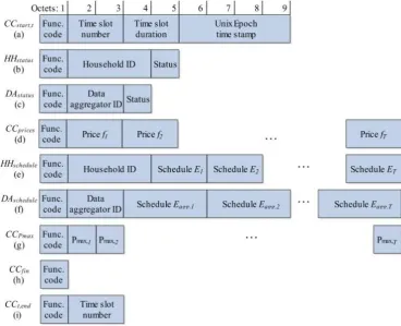
The protocol data exchange consists of 9 types of messages, based on the algorithm’s functionality described in [11]. Support for household/aggregator mechanisms for registration or data security is not provided, as it is assumed that additional network technologies like the RADIUS protocol and virtual private networks will be adopted in the communication system. Each message is identified by a 1-byte long function code (figure 3). The control center starts by broadcasting CCt,start message (figure 3(a)), announcing the beginning of the new time

slot. The message fields are time slot number, time slot duration and time stamp, used as time reference. After the reception of CCt,start, the households are required to report their operational status with HHstatus message to

their assigned data aggregator (figure 3(b)). The message contains the 3-byte household ID (allowing a total of 16 777 215 unique participating households) and a status field, indicating if the house is ready to proceed with the current time slot, or an internal error has occurred, preventing the household from participating. DAstatus

message is generated when a certain DA received all the expected HHstatus messages from the connected

households (figure 3(c)). DAstatus is used to notify the CC that the aggregator is ready and await the price vector

message. It contains aggregator ID field (maximum of 65 535 unique aggregators) and a status field, indicating if the aggregator is ready to proceed with the current time slot, or an internal error has occurred, preventing it from participating. After the reception of all expected DAstatus messages, the CC broadcasts CCprices to all the

aggregators with positive DAstatus, which in turn broadcast it to their assigned HHs. The message contains the

energy pricing information over the time horizon T. Each household EMS solves the optimization problem and generates consumption schedule for its controllable appliances, based on the received pricing information and the user-input preferences. The collective schedule for the time horizon T is then sent to the CC using the

HHschedule message (each time slot energy consumption field has 2-byte length allowing a total energy

consumption representation of 216 Wh or 65.535 kWh). The aggregated energy schedule message (DAschedule)

contains the aggregated energy consumption vectors of various households for the time horizon T (3 bytes per time slot, allowing 16.7 MWh). It also contains the ID of the data aggregator (2 bytes). After collecting all the expected schedules, the CC converts and compares the consumption schedules with the renewable power generation forecasts, obtaining the difference Vdiff. If the difference is acceptible, the schedules are marked as

final by sending CCfin message. Otherwise, a CCPmax message is broadcasted, starting a new iteration and

containing the power consumption limitations over the time horizon T. After its arrival at a DA, the CCPmax is

then broadcasted again to the assigned HHs, which in turn solve their optimization problems using the new consumption limits. Note that, if an EMS is unable to find a feasible solution, the previous successful schedules will be used until the new Pmax consumption limits are received in the next iteration.

The message CCfin (figure 3(h)) is sent by the CC in three cases: 1) if the difference between consumption

and generation is lower than the predefined level; 2) an optional and predefined maximum iterations number is reached; and 3) CCt,end message has been generated. In those conditions, the CC marks the schedules as final and

notifies the households with CCfin message. The CC announces the upcoming end of the current time slot using

CCt,end (figure 3(i)). The message is generated at time td – td/20, i.e. 5% of the time slot duration period is left

after CCt,end has occurred. It is used to ensure a sufficient time buffer and prevent events from previous time slot

to interfere with a new one. If there is undergoing algorithm iteration, the CC cancels it, marking the generated schedules from the previous algorithm iteration as finalized and sends CCfin announcement message.

As the CC and DAs collect status and energy scheduling information during each time slot, several message timeout timers have been implemented in their application logic to avoid infinite waiting. The timers’ values must be selected carefully as the reason for a delayed message may be longer than usual run of the household’s optimization solver or network congestion, causing large number of TCP retransmissions. After a timer expires, the expected but not responding HHs or DAs are excluded by their assigned DA or CC respectively, forcing the mechanism to operate with incomplete information (in this case, the last consumption schedule to have been submitted successfully by a HH or a DA will be used).

Assuming an IPv6 network segment with a maximum transmission unit (MTU) of 1500 B at the IP layer, the largest TCP maximum segment size (MSS) will be 1440 B [16], i.e. CCprices/CCPmax/HHschedule/DAschedule can

theoretically carry information for up to T = 719/1439/718/479 time slots respectively, without being segmented and causing additional lower layer protocol overhead. Table I summarizes the message lengths at the application layer for four common time slot durations td = 5, 15, 30 and 60 minutes (with one day receding horizon), as well

as the application layer protocol data unit (PDU) efficiency, Deff = (PDUL5/PDUL2).100%, after the

encapsulation by TCP, IPv6 and IEEE 802.3 Ethernet. Ethernet is chosen to represent the link layer as it offers integration with fiber optics, wireless technologies (e.g. IEEE 802.16 WiMAX) and powerline communications (PLC).

TABLEI

MESSAGE LENGTHS AND PAYLOAD EFFICIENCY FOR 24-HOUR RECEDING HORIZON

Message type

td = 5 min,

T = 288

td = 15 min,

T = 96

td = 30 min,

T = 48

td = 60 min,

T = 24 PDUL5

(B) Deff, % PDUL5

(B) Deff, % PDUL5

(B) Deff, % PDUL5

(B) Deff, % CCt,start 9 10.34 9 10.34 9 10.34 9 10.34

HHstatus 5 6.03 5 6.03 5 6.03 5 6.03

DAstatus 4 4.88 4 4.88 4 4.88 4 4.88

CCprices 577 88.09 193 71.22 97 55.43 49 38.58

HHschedule 580 88.15 196 71.53 100 56.18 52 40

DAschedule 867 91.75 291 73.44 147 65.33 75 49.02

CCPmax 289 78.75 97 55.43 49 38.58 25 24.27

CCfin 1 1.27 1 1.27 1 1.27 1 1.27

CCt,end 3 3.7 3 3.7 3 3.7 3 3.7

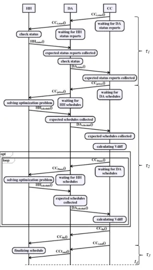
Fig. 4 Simplified message flow for a single time slot

IV.PERFORMANCE PARAMETERS

As the algorithm is distributed and strongly relies on the communication infrastructure, it is important to study its performance under realistic scenarios. Communication losses among participants can be caused by wide variety of complex network conditions. Therefore, it is important for a unified parameter, reflecting the performance, to be defined.

Let the intervals τ1, τ2, τ3 divide a time slot t into three phases. The first phase τ1 corresponds to the duration

from the time slot start CCstart,t and the reception of all DAschedule messages (figure 4). The second phase τ2

denotes the time available for iterations (starting at the generation of CCprices message) and τ2 = td - τ1 - τ3. The

third phase τ3 represents the time buffer after the time slot end announcement CCend,t. Let τit denote the time

needed for completing a single iteration, i.e. τit represents the time interval between the consecutive sending of

τ

τ

τ

CCprices or CCPmax messages. Then the relation between the available iterations it for each time slot and τit is given by: 2 t it i







As the performance of the algorithm depends on it, the following parameters are a subject of the current study

- packet loss, bit and packet error rates, and end-to-end delays. The delays caused by the application logic of HHs, DAs and the CC are also discussed.

A. Packet loss

As in the current study TCP is used as the underlying transport protocol, high packet loss due to network congestion can cause large number or retransmissions, lowering it and possibly leading into timer expirations and loss of scheduling information. Thus, it is essential to evaluate the algorithm’s performance in cases with heavy background traffic conditions, representing a congested network with multiple smart grid communication services. A simple way of measuring TCP packet loss is to divide the number of retransmitted packets by the total number of generated packets:

 r

loss tot

n P

n

B. Bit and packet error rates

The bit error rate (BER) is the number of bit errors divided by the total number of received bits during a time interval. Similarly, the packet error rate (PER) is the error packets divided by the total number of received packets. The relationship between PER and BER in a single network segment can be simply expressed with:

1 (1 )

   PL

PER BER

where PLis the packet length in bits. The WAN is assumed to use high-performance fiber-optic channels, which

are characterized by very low bit error rates in the order of 1e-9 [17]. For a 12000-bit packet (1500 bytes), having BER in that order will result in PER ≈ 1.2e-5 or 0.0012% retransmission rate due to packet errors. The use of bit error correction mechanisms reduces PER further, thus such value is considered negligible for having an impact on the protocol’s performance. However, the wide range of network solutions for the NAN infrastructure include power line carrier technologies, which are more affected by a transmission channel noise, interference, distortion, bit synchronization problems, etc. The experimental results from [18] show PER reaching a value of 5e-2 in links between PLC modems and MV/LV transformers. The NAN PLC performance evaluation models developed in [19] consider a uniform distribution of PER in the interval (0, 5.6e-2). Such rates can lead into high TCP retransmissions and are of interest in the current study.

C. Network delay

The total end-to-end network delay dete is defined as:

1 1 1 1

   

















ete q proc tr prop

h h m m

d

d

d

d

d

where H is the number of hops between source and destination, M is the number of communication links and M

= H + 1; dq is the queuing delay at hop h and dhproc is the packet processing delay at hop h. The transmission

delay is dmtr= PL / Rm, where PL is the packet length (in bits) and Rm is the transmission rate of the link m (in

Mbps). Propagation delay of a link is calculated as dmprop = δm / s, where δm is the link length and s is the

propagation speed of the medium. As the WAN is assumed to use fiber-optic medium (s≈ 200000 km/s), the

link propagation delay in this study will be considered dprop, WAN = 5 µs/km. The NANs cover limited

geographical regions of up to 10 km in range, hence their propagation delays are neglectable.

During the aggregation process, the HHschedule messages are discarded after the energy consumption schedules

have been extracted and then encapsulated into packets with different PL size (as roughly DAschedule ≈

1.5HHschedule in size, Table I). Therefore, for those messages a three-component total network delay is to be

the time period between DAschedule being sent and its reception at the CC. The third term corresponds to the delay

caused by the aggregation process of the energy schedules.

D. Data aggregation delay dagg

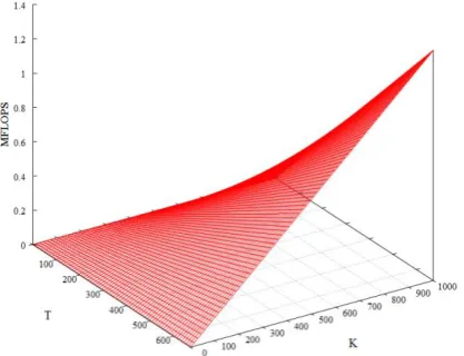
With each arrival of a HHschedule message, the DA populates E = K×T matrix, with each row representing an

energy consumption vector E'k= [Ek1, Ek2,…, EkT], k ∈ K. After all messages are collected, the matrix is then

transformed into an output vector E'agg,n = [ΣEk1, ΣEk2,…, ΣEkT], k = 1..K, containing the collective energy

schedule of the HHs in the designated NAN. E'agg,n is derived by premultiplying the matrix by the transpose of

1K, thus the computational cost is equal to K(2T – 1) FLOPS [22]. Figure 5 depicts the MFLOPS requirements

using a maximum of T = 672 time slots (one week receding horizon, td =15 minutes) and a maximum of K =

1000.

Fig. 5 Computational requirements for the energy schedules aggregation

It is clear that the computational requirements of the proposed aggregation approach are substantially lower than the capabilities of modern complex instruction set computing (CISC) architectures. Therefore, a reduced instruction set computing (RISC) device is chosen to represent the DA’s hardware in the simulation models,

offering lower costs and higher energy efficiency and performance in terms of FLOPS/W. BeagleBoard,

Raspberry Pi and Chumby One are among the suitable Advanced RISC Machine-based (ARM-based) boards. In

[20], the authors present benchmark results of Cortex-A8 BeagleBoard with performance of 23.376 MFLOPS.

Bearing it in mind, the aggregation process delay with bounds T = 672 and K = 1000 results in dagg∈ [8.6×10-5,

57.45] ms.

E. Household’s computational time

Because the HHs are not synchronized, optimization runs in the different households are not executed at the same time. In the current implementation [11], a single household run requires ≈0.38 seconds to generate the consumption schedules for a time horizon of 24 hours, divided into 96 time slots, on a PC with Intel Core i7-2700 CPU. However, solving the optimization problem on embedded hardware will require significantly longer computational times. Assuming RISC design is implemented, with each household EMS having ARM Cortex-A9 CPU, [21] shows an execution time ratio of 8.4 between i7-2700 and Cortex-Cortex-A9 on a SPEC INT desktop workload benchmark. Therefore, a household EMS will require an average of 3.19 seconds in order to solve the optimization problem using the RISC CPU. In order to take into account the fact that computational times vary due to the different household appliance types and their numbers, the delay caused by the solver is set to a uniform distribution in the interval (2.5s, 4s) for each optimization run with regard to the introduction of those computational time uncertainties. The same relation is used when evaluating the impact of multiple time slot durations (and respectively receding time horizons) during the simulation runs, described in Section V.

F. Central controller’s computational time

The utility’s server infrastructure is assumed to have always sufficient computational resources, thus the caused delays by the processes of generating CCprices and CCPmax messages are negligible. As the CC relies on

V. CASE STUDY

In this section, the simulation test cases, designed to evaluate the impact of the aforementioned network performance parameters, are described. The HH, DA and CC applications are written in C++ and the network models are built within the OMNeT++ 4.6 environment [23], using the INET 2.6.0 framework [24]. The simulation runs are performed on a virtualization server with Intel Core i5-4570 and 16 GB DDR3-1600 RAM.

The WAN network topology consists of 10 core routers connected in a ring topology, allowing two independent routes from HHs to CC. Varying number of connected NANs, respectively DAs, are considered through the different scenarios. Figure 6 shows the studied network topology for N = 10. The maximum hop

count is Hmax = 20 and the minimum is Hmin = 5 (taking into an account the additional two hops added by the

DA). The WAN propagation delay dprop is set to 50µs per link (10 km length) with BER values of 1e-9.

Fig. 6 Test network for N = 10

All simulation runs are performed with equivalent TCP-related mechanisms and settings. Nagle’s algorithm is disabled, due to the absence of short TCP packet floods (all short messages, shown in Table I, are generated at a low rate with relatively long pauses). The default TCP MSS is used (536B), the flavor is TCP New Reno (the SACK mechanism is absent) and the Limited Transmit algorithm is enabled.

The following simulation scenarios have been developed.

A. Best case scenario

A benchmark scenario is implemented, without considering the negative impact of PER and background traffic. The packet queues are modelled as infinite buffers to prevent any packet loss. We assume that the DAs are situated at the same location as the edge routers, thus their links are modelled as Gigabit Ethernet, in order to avoid any potential bottlenecks. Nevertheless, we do consider the computational and network delays in a background traffic-free environment. The scenario’s aim is to evaluate the relationship between the average number of available iterations per time slot i_t , the number of aggregators N and the time slot duration td. As it is

assumed that the WAN and NANs are also used for a variety of other smart grid applications and services, limited data rates, RWAN and RNAN, are taken into account. The number of households per data aggregator (K)

may vary significantly due to areas with different population densities and/or the consumers’ willingness to participate in the mechanism. Therefore, the impact of K is also considered.

B. Packet error rate scenario

As discussed in Section IV, NAN communication technologies are more likely to introduce high PERs, leading into TCP retransmissions and deterioratingi_t. Given the message collection process of a DA, the performance is expected to decrease significantly with the increase of K, due to the higher probability of errored-packets occurring. The performance in the scenario is evaluated by varying the PER values of NAN links in the range of [1e-9, 1e-2].

C. Background traffic scenario

priority over the DR protocol at the corresponding router interfaces. Wide Area Measurement System (WAMS) application is chosen to represent the background traffic mainly for two reasons: 1) Phasor Measurement Units (PMUs) generate IEEE C37.118 messages at high constant bitrates, and 2) they are characterized by very high intolerance to packet delays [25]. It is assumed that in the future, PMUs will be deployed not only in the transmission system, but also in the distribution system, to better manage power quality, particularly with large scale deployment of distributed generation [25], [26].

A single IEEE C37.118 PMU traffic source is placed in each NAN, connected to the corresponding edge router. As in the case of a PMU placement in the distribution grid, utilizing high number of measurement channels is unlikely. Therefore, each PMU is set to generate measurement samples from a single channel. According to the IEEE C37.118 standard [27], the resulting generated data will be 24 bytes per sampling period (76 bytes with lower layers protocol overhead). Assuming the frequency of the AC current is 50 Hz, a sampling period of 20ms (rate 50 measurements/s) is chosen, resulting in 30.4 kbit/s constant bitrate stream. As td is 15

minutes, the number of generated C37.118 packets is 45000 per PMU per time slot, resulting in total traffic volume of 3.283 GB for 24 hours.

As the future smart grids will rely heavily on PMU data to maintain the grid’s stability and integrity, a strict traffic prioritization has been implemented in the simulation model. A multifield classifier is used at the routers’ ingress interfaces to distinguish traffic flows based on source address and destination port, implemented by an external XML script. The priority queues use drop-tail packet dropping strategy. The high priority PMU streams have Diffserv Expedited Forwarding per-hop behavior, [28], with 99% reserved bandwidth, guaranteed by a priority scheduler. Such priority scheduling and forwarding aims at minimizing the C37.118 packet loss and end-to-end delay, as well as evaluating the robustness of the proposed protocol message exchange. The interface queues have fixed capacity of 10 frames. Setting small queue lengths is aimed towards avoiding the “bufferbloat” phenomenon, initially described in RFC 970 [29].

The NAN links in the scenario have fixed data rates of RNAN = 1 Mbit/s, while RWAN values vary between 25

and 350 kbit/s. The other simulation parameters are td= 15, T = 96, N = 10, K = 100.

VI.SIMULATION RESULTS

Each value of i_t is obtained as the average result of 10 simulation runs with differing seeds of the Mersenne Twister pseudorandom number generator.

A. Best case scenario

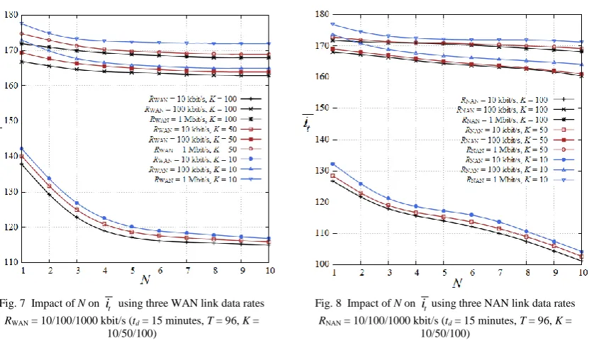
Figure 7 depicts the impact of the number of data aggregators N and the number of households per aggregator

K, on the average i_t , using three different data rates for the WAN links, RWAN = 10 / 100 / 1000 kbit/s. The time

slot duration td is 15 minutes and the time horizon T is 96 time slots large. The data rate of all NAN links is

constant, RNAN = 1 Mbit/s. The lowest average number of available iterations is 115, in the case of 10 kbit/s

links, N = 10 and K = 100 (1000 simulated households), and the highest is 179, in case RWAN = 1 Mbit/s, N = 1

and K = 10 (100 simulated households). Further increase in RWAN does not contribute to achieving higher

performance, e.g. in the case of N = 1, K = 10 and RWAN = 10 Gbit/s, the maximum number of available

iterations is the same as in RWAN = 1 Mbit/s, it = 179. Furthermore, there is an overall minor decrease in it

while using data rates over 100 kbit/s. However, in the case of RWAN = 10 kbit/s, the results indicate significant

reduction compared to RWAN = 1 Mbit/s. The percentage performance reduction for K = 10, 50, and 100 varies in

the ranges of 19.55% to 31.98%, 18.86% to 31.36% and 18.60% to 31.54% respectively, mainly due to the larger queueing delays. The small variations in these performance drops suggest predictability, assisting the network design.

Figure 8 shows the impact on i _t using three different data rates for the NAN links RNAN = 10 / 100 / 1000

kbit/s. The results indicate similar behaviour as in the previous figure, with i_t mainly affected by the lowest data rate of 10 kbit/s. The lowest and highest achieved performances are 101 and 178 iterations respectively.

As noted before, the presented results for the current scenario are obtained under the assumption that each DA is situated at the same location with its corresponding edge router, thus the link between them is modelled as Gigabit Ethernet. If a DA is positioned at a remote location and is using the same NAN communication technologies as the households in order to connect to an edge router, a considerable reduction in performance is observed. For example, changing the link’s data rate to 100 kbit/s for N = 10, K = 100 and RWAN = RNAN = 1

Fig. 7 Impact of N on i_t using three WAN link data rates RWAN = 10/100/1000 kbit/s (td = 15 minutes, T = 96, K =

10/50/100)

Fig. 8 Impact of N on i_tusing three NAN link data rates RNAN = 10/100/1000 kbit/s (td = 15 minutes, T = 96, K =

10/50/100)

The results using four different td are depicted in figure 9. The time slot duration values are chosen according

to the most common ones, found in the smart grid literature. The receding horizon is 24 hours long, the number of households per DA is K = 100, and the lengths of the protocol messages are modified as stated in Table I. The results clearly show significant differences in terms of performed iterations during the simulation runs. Using the longest time slot interval (td = 60 minutes), the achieved maximum it is 934 iterations in comparison to only

41, in the case of td = 5 minutes. Further, the network traffic generated by the protocol for 24 hours (figure 9),

obtained during the simulation run with td = 5 minutes exceeds the 60-minute one by nearly 129%. Nonetheless,

shorter time slots allow larger time resolution for scheduling interruptible household appliances, thus substantially increasing the algorithm’s flexibility during periods of peak loads and low local renewable energy generation. In terms of the impact of N oni_t, the difference in iterations between N = 1 and N = 10 for td = 5 / 15

/ 30 / 60 minutes is i_t = 1 / 4 / 5 / 7, respectively, suggesting that the number of data aggregators does not

contribute significantly to changes ini_t when sufficient link data rates are provided.

Fig. 9 Impact of four different values of td on i_t(RNAN = 1 Mbit/s, RWAN = 1 Mbit/s, N = 1 and 10, K = 100), as well as the total generated

network traffic for N = 10 B. Packet error rate scenario

Fig. 10 Impact of PER in NAN links on i_t (N = 10, td = 15 minutes, RNAN = 1 Mbit/s, RWAN = 1 Mbit/s)

If network technologies, unable to provide low PERs, are used, this can be interpreted as a “weak spot” in the proposed architecture, due to the specifics of the aggregation process – each DA attempts to collect all consumption schedules before a timer expires (otherwise being forced to send incomplete information to the CC). Nevertheless, when K is kept low, the protocol is still able to achieve satisfactory number of iterations.

C. Background traffic scenario

The obtained results for i_t during the simulations of the third scenario are summarized in figure 11. As the WAN network has ring topology, the bottlenecks in the implementation are the positioned close to the CC core routers. Due to congestion at those routers, the protocol is unable to achieve any iterations only in the case of

RWAN = 25 kbit/s. Increasing RWAN to 50 kbit/s allows the protocol to achieve 4 iterations. However, such a low

number is unlikely to be sufficient for a successful peak load reduction, as the CC will be forced to increase drastically the rate at which Pmax vector values change in each iteration. This in turn will result in each EMS

finding an optimal schedule for each appliance closer to the start of the defined by the household residents energy consumption time window (as the EMS respects the residents’ own preferences, in order to minimize the discomfort caused by the load-shifting). The maximum i_t = 172 is observed at RWAN = 350 kbit/s. Further

increase of the data rate does not contribute to higher i_t , as then the main source of delays are the data aggregation processes and the household energy consumption optimization times.

Fig. 11 Impact of PMU background traffic on i_t

The PMU traffic results for packet loss, average queueing time d_qand maximum queueing time dq,max of the

core routers, as well as the average end-to-end delay d_ete, are summarized in table II. The high values of the four parameters when RWAN is under 125 kbit/s are due to the lack of sufficient network capacity, despite the

traffic prioritization. In such severe network congestion conditions, the low capacity of interface queues (10 frames) is crucial for maintaining lower d_q of the high priority traffic, which in turn contribute to lower dete.

For example, changing the queue frame capacity to 100 in the case of RWAN = 100 kbit/s, shows dete= 245 ms or

TABLEIII

BACKGROUND PMU TRAFFIC RESULTS

RWAN (kbit/s)

Parameter

25 50 75 100 125 150 175 200 225 250 275 300 325 350

Ploss, % 68.82 47.64 26.78 7.73 0.36 0.16 0.07 0.02 0.005 0.003 0.002 0.0011 0.009 0.00044 q

d , ms _{107 44 21 6.2 1.4 0.63 0.48 0.25 0.16 0.21 0.21 0.2 0.19 0.17}

,max q

d , ms _{189 126 94 80 58 51 41 27 20.4 20.3 19.6 18 14 12.1}

ete

d , ms 261 186 95 41 18 15.5 13.7 11.6 10.6 9.8 9.3 8.7 8.1 7.9

VII. CONCLUSION

The current study addresses the problem of distributed and communication-enabled demand-side load shifting of residential households. A model of an application layer protocol has been presented, aimed at enabling residential load shifting by taking an advantage of the distributed communication nature of the integrated algorithm within it. Extensive simulation scenarios have been developed, in order to evaluate the main performance metric (average number of iterations per time slot) against the network parameters. The results indicate high scalability and robustness of the approach, showing satisfactory performance even during the worst-case scenarios. Furthermore, no strict technological requirements need to be defined for the communication infrastructure, allowing the choice for infrastructure to be flexible, with possible differences between the NAN implementations.

REFERENCES

[1] K. C. Budka, J. G. Deshpande, M. Thottan, Communication Networks for Smart Grids, Springer-Verlag London, 2014.

[2] M. G. Seewald, “Scalable Network Architecture based on IP-Multicast for Power System Networks”, in 2014 Innovative Smart Grid Technologies Conf. (ISGT’2014), Washington, USA, pp.1-5, Feb. 2014. [3] F. Baker and D. Meyer, “Internet Protocols for the Smart Grid”, RFC 6272, June 2011.

[4] A. Giusti, M. Salani, G. A. Di Caro, A. E. Rizzoli and L. M. Gambardella, “Restricted Neighborhood Communication Improves Decentralized Demand-Side Load Management”, IEEE Trans. Smart Grid, vol.5, no.1, pp.92-101, Jan. 2014.

[5] M. Pipattanasomporn, M. Kuzlu, S. Rahman and Y. Teklu, “Load Profiles of Selected Major Household Appliances and Their Demand Response Opportunities”, IEEE Trans. Smart Grid, vol.5, no.2, pp.742-750, Mar. 2014.

[6] C. Rottondi and G. Verticale, “Privacy-Friendly Appliance Load Scheduling in Smart Grids”, in 2013 IEEE Int. Conf. on Smart Grid Communications (SmartGridComm’2013), Vancouver, Canada, pp.420-425, Oct. 2013.

[7] P. Chavali, P. Yang and A. Nehorai, “A Distributed Algorithm of Appliance Scheduling for Home Energy Management System”, IEEE Trans. Smart Grid, vol.5, no.1, pp.280-290, Jan. 2014.

[8] A.-H. Mohsenian-Rad, V. Wong, J. Jatskevich and R. Schober, “Optimal and Autonomous Incentive-based Energy Consumption Scheduling Algorithm for Smart Grid”, in 2010 Innovative Smart Grid Technologies Conf. (ISGT’2010), Gaithersburg, USA, pp.1-6, Jan. 2010.

[9] A. Mahmood, M. N. Ullah, S. Razzaq, A. Basit, U. Mustafa, M. Naeem and N. Javaid, “A New Scheme for Demand Side Management in Future Smart Grid Networks”, in Procedia Computer Science, vol.32, pp.477-484, 2014.

[10] K. Mets, F. De Turck and C. Develder, “Distributed smart charging of electric vehicles for balancing wind energy”, in 2012 IEEE Int. Conf. on Smart Grid Communications (SmartGridComm’2012), Tainan, Taiwan, pp.133-138, Nov. 2012.

[11] M. Ivanov, “Household Appliances Scheduling for Efficient Renewable Energy Consumption”,Journal of Emerging Trends in Computing and Information Sciences, vol.6, no.7, pp.355-362, Jul. 2015.

[12] D. Çınar, G. Kayakutlu, “Forecasting Production of Renewable Energy Using Cognitive Mapping and Artificial Neural Networks”, in 19th Int. Conf. on Production Research (ICPR-19), Valparaiso, Chile, Jul. 2007.

[13] J. Zhang, B.-M. Hodge, A. Florita, S. Lu, H. F. Hamann and V. Banunarayanan, “Metrics for Evaluating the Accuracy of Solar Power Forecasting”, 3rd Int. Workshop on Integration of Solar Power into Power Systems, London, England, Oct. 2013.

[15] W.-Y. Chang, “A Literature Review of Wind Forecasting Methods”, Journal of Power and Energy Engineering, vol.2, pp.161-168, Apr. 2014.

[16] D. Borman, “TCP Options and Maximum Segment Size (MSS)”, RFC 6691, Jul. 2012. [17] B. E. A. Saleh, M. C. Teich, Fundamentals of Photonics, 2nd Ed., Wiley-Press, Feb. 2013.

[18] C. Males, V. Popa, A. Lavric, I. Finis and S. cel Mare, “PLC Performance Evaluation Through a Power Transformer Using PRIME”, in Buletinul AGIR, no.3, pp.257-262, Jun-Aug. 2012.

[19] D. F. Ramirez, S. Cespedes, C. Becerra and C. Lazo, “Performance Evaluation of Future AMI Applications in Smart Grid Neighborhood Area Networks”, in 2015 IEEE Colombian Conf. on Communications and Computing (COLCOM), Popayan, Colombia, pp.1-6, May 2015.

[20] K. R. Hoffman, P. Hedge, “ARM Cortex-A8 vs. Intel Atom: architectural and benchmark comparisons”, Technical Report, University of Texas, 2009,

Available online: http://caxapa.ru/thumbs/229665/armcortexa8vsintelatomarchitecturalandbe.pdf

[21] E. Blem, J. Menon and K. Sankaralingam, “Power Struggles: Revisiting the RISC vs. CISC Debate on Contemporary ARM and x86 Architectures”, in 19th IEEE Int. Symposium on High Performance Computer Architecture (HPCA0-19), Shenzhen, China, Feb. 2013.

[22] R. Hunger, “Floating Point Operations in Matrix-Vector Calculus”, Technical Report version 1.3, Technische Universität München, 2007.

[23] OMNeT++ 4.6 Simulation Environment, http://www.omnetpp.org/

[24] INET 2.6.0 Framework for OMNeT++/OMNEST, http://www.inet.omnetpp.org/

[25] K. V. Katsaros, B. Yang, W. K. Chai and G. Pavlou, “Low Latency Communication Infrastructure for Synchrophasor Applications in Distribution Networks”, in Proc. IEEE Int. Conf. on Smart Grid Communications 2014 (SmartGridComm’14), pp.392–397, Nov. 2014.

[26] M. Paolone, A. Borghetti and C. A. Nucci, “A Synchrophasor Estimation Algorithm for the Monitoring of Active Distribution Networks in Steady State and Transient Conditions”, in Proc. of the 17th Power Systems Computation Conference (PSCC’2011), Stockholm, Sweden, pp.1-8, Aug. 2011.

[27] IEEE Standard for Synchrophasors for Power Systems, IEEE Std. C37.118 –2005.

[28] B. Davie, A. Charny, J.C.R. Bennett, K. Benson, J.Y. Le Boudec, W. Courtney, S. Davari, V. Firoiu and D. Stiliadis, “An Expedited Forwarding PHB (Per-Hop Behavior)”, RFC 3246, Mar. 2002.