EXPERIMENTAL EVALUATION AND SET-UP OF A NEW APPARATUS
DESIGNED FOR TRANSITIONAL FLOW EXPERIMENTS
Sakhr ABU-DARAGxand Dalibor ROZEHNALxx
Abstract:Experimental exercise has been conducted to validate the capability of a new test apparatus. The test stand has been designed and constructed at the laboratory of aerodynamics, University of Defence to carry out the experimental investigation of transitional flow prediction and development over flat plate. The test facility consists of a rectangular duct set on the suction side of air source apparatus. The working section is 2 m long with a cross section of 0.44 m in width and 0.25 m in height. The exercise is performed into two stages. In the first stage, the basic parameters such as freestream velocity, turbulence intensity and pressure gradient in streamwise direction were measured and manipulated to set-up acceptable values. Second stage of the exercise, the bottom wall of the test section was used as a flat plate model to conduct turbulent boundary-layer experiment. The characteristics of the boundary layer obtained by using the apparatus are represented by a qualitative and quantitative agreement with those predicted by boundary-layer theory for turbulent boundary layer while more improvements seems to be required to satisfy the rules of boundary layer stability experiments. The results are show a fair agreement for mean velocity profile, U, boundary layer thickness, , momentum thickness,ș, and skin friction coefficient, Cf
1. I
NTRODUCTION.
Keywords: Transitional flow; Turbulence intensity; Transitional boundary layer; Momentum thickness; Skin friction coefficient
For more than a century, the problem of transition to turbulence has been an area of interest to researchers. This interest is due to, firstly, the necessity of solving practical problems, related, for instance, to the task of controlling boundary layer, in order to decrease the drag of aircrafts and vessels. Secondly, the study of transition to turbulence is an integral part of a more fundamental problem, ((i.e. the description of the very phenomenon of turbulence)).
In the end of the nineteenth century, Reynolds [1] and Rayleigh [2] hypothesized that the reason of transition from laminar flows to turbulent ones is the instability of the former. In other words, an increase of the intensity of waves within an instable boundary layer leads to the destruction of laminar flows. In 1924, Heisenberg [3] laid the
x Sakhr Abu-Darag, University of Defence, Kounicova 65, 662 10 Brno, Czech Republic, e-mail:
xx Dalibor Rozehnal, University of Defence, Kounicova 65, 662 10 Brno, Czech Republic. e-mail:
foundation for developing a linear theory of hydrodynamic instability. First computations of the boundary layer stability were performed much later - between the end of the 1920s and the beginning of the 1930s by Tollmien [4] and Schlichting [5-7]. Later, Taylor [8] proposed another hypothesis, according to which transition to turbulence is caused by fluctuations within the outer flow that lead to the local separations of the boundary layer. Until the 40-th, doubts about the validity of the stability theory prevailed, for the experimental evidence of that period was in favour of the Taylor hypothesis. In particular, the experiments by Dryden [9-10], who applied a novel for that time technique: measurements by the use of thermo-anemometer, were supportive of the Taylor hypothesis. In 1948, for the first time, Schubauer and Skramstad [11] found out how fluctuations within the boundary layer play the key role in the destruction of the laminar flow regime. It is known that transition in boundary layer that flows in turbomachines and aerospace devices is affected by various parameters, such as freestream turbulence, pressure gradient and separation, Reynolds number, Mach number, turbulent length scale, wall roughness, streamline curvature and heat transfer. Due to this variety of parameters, there is no existing mathematical model that can predict the onset and length of the transition region. In addition to the influence of these parameters upon transition origination, the poor understanding of the fundamental mechanisms which lead initially small disturbances to transition may also causes this lack.
Considering a rigorous theory of the laminar-turbulent transition, then such an adequate formal theory, in the first place, has to allow the description of the evolution of instability: its appearance, development, the observable destruction of the laminar flow, and the final transition to a fully developed turbulent flow. Solving such a problem involves great mathematical difficulties. In fact, in spite of all efforts, until today there no fundamental theory of transition, just experiments and correlations that try to predict the final onset of fully turbulent flow.
The objective of the present work is to evaluate experimentally the capability of a new apparatus designed for conducting experiments of transitional boundary layer flows over a flat plate with zero pressure gradient.
2. EXPERIMENTAL FACILITY AND MEASUREMENT TECHNIQUES
2.1. Test facility for the investigationthe tunnel. The first mesh is 0.375 0.375 mm with a wire diameter of 0.10 mm and free area 62 % was installed 35 cm downstream before the trailing edge of the plate while the second mesh is 0.50 0.50 mm with a wire diameter of 0.14 mm and free area 61 % was installed at the end of the duct. The wall-normal pressure distribution at different locations represents in Figure 3 and 4. Smooth rounded entrance with ellipse shape (a=230 mm and b=140 mm) was attached to the duct at the inlet in order to reduce the effect of the abrupt entrance condition on the test stand characteristics. The most influenced characteristics by the entrance geometry are entrance length, local friction factor, pressure gradient variation in the entry region, and the laminar to turbulent transition for the flow in the duct [12].
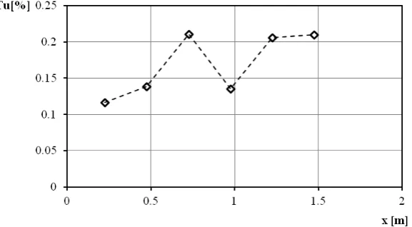
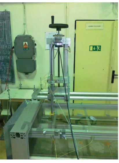
The turbulence level in the test section is reduced by installing damping screen upstream between the entrance and the duct. The specification of the mesh is 0.09 0.09 mm with a wire diameter of 0.05 mm and free area 40 %. Figure 5 illustrates the turbulence intensity distribution along the flat plate. Although the apparatus is recommended to have a longitudinal fluctuation level less than 0.1% in the streamwise direction and less than 0.2% in the spanwise and wall-normal direction, it is clear that the turbulence level average in the duct is approximately 1.5%. A computer-controlled two-axis traversing system indicated by Figure 6 permits to measure in streamwise and wall-normal coordinates system, while the signals are recorded using Lab-VIEW with a 16-bit NI PCI-6040E data acquisition card.
Figure 1: Experimental facility
2.2. Data acquisition
hot wire was digitized at a sampling frequency of 20 kHz using 16 bit analogue to digital converter for number of samples equal to 2.1016.
2.3. Flat plate set-up
The bottom wall of the duct is used as a model for the plate at zero incidence to study the boundary layer characteristics and the influence of the heat transfer upon transition process. The material of the plate is hardened commercial duralumin sheet consist of Al, Cu4 and Mg. Thickness of the plate is 6 mm and the entire allowable working length is 152 mm due to the instruction of the downstream screen and effect of the entrance.
Figure 2: Streamwise mean velocity distribution outside of the boundary layer
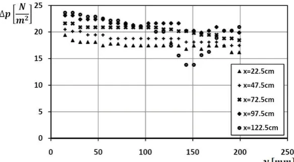
Figure 3: The wall-normal pressure distribution at different locations
2.4. Heating system
by a thermocouple mounted in the traversing mechanism. Thin film heat flux sensors fixed (taped) on the plate surface at constant interval of 250 mm is used to read the temperature on the plate along the entire working length. Moreover, permanent electronic thermocouples are installed along streamwise direction with the same previous sensors interval to deduct the free stream temperature at different locations
Figure 4: Pressure distribution along the plate
Figure 6: Traversing mechanism
3. THEORTICAL
BACKGROUND
Considering flow over a flat plate with a zero pressure gradient, the exact solution for laminar boundary layer which proposed by Blasius gives the thickness of the boundary layer [13] and [14]
x
x
x
Re
0
.
5
G
(1)with,
Q
x
U
x f
Re
(2)Where
x
is the distance along the flat plate measured from the leading edge;G
is the thickness of the boundary layer; U is the freestream velocity of the air;Q
is the kinematic viscosity of the air; and RexFor turbulent boundary layer, the thickness cannot be exactly determined. However, it can be estimated by using the momentum-integral equation given by Kármán [15]
is Reynolds number.
dx
dU
U
U
dx
d
w 2
T
G
*U
W
(3)
with considering power-law profile suggested by the following relations
y
nU
u
1
¸
¹
·
¨
©
§
G
(4)
D
{
1
2
1
2
2n
n
n
U
V
(5)where
W
w is the wall shear stress,U
the mass density of the air,x
is the distance in streamwise coordinate, U is the freestream velocity in a power-law velocity distribution,V
is the average velocity,D
is the ratio of the average velocity to the freestream velocity,T
is the momentum thickness,G
* is the displacement thickness,G
is the boundary-layer thickness, andy
is the wall-normal distance from the plate. The momentum thickness and the displacement thickness are given, respectively, by
dy
U
u
U
u
³
¸
¹
·
¨
©
§
GT
01
(6)and
dy
U
u
³
¸
¹
·
¨
©
§
GG
* 01
(7)the thickness of the boundary layer is realized by integration of Eqs. (4) and (5) in the momentum-integral equation as
5 / 1
Re
xax
x
#
G
(8)where
a
a
n
(9) Moreover this relation which relatesa
to the power lawn
can be established as
°
°
¿
°
°
¾
½
°
°
¯
°
°
®
»¼
º
«¬
ª
»
¼
º
«
¬
ª
5 / 4 2 5 / 7 23
2
1
2
1
2
07842
.
0
n
n
n
n
n
n
a
(10)According to this relation for any given
n
, the numerical value ofa
can directly be determined.4. RESULTS AND
DISCUSSION
4.1. Characterization of boundary layersThere are many techniques in literature that characterize the boundary layer, to determine whether it is laminar, transitional or turbulent. Among those techniques, the variation of boundary layer integral parameters such as momentum thickness, friction coefficient and shape factor within the boundary layer or the prediction of the nature of the velocity profile inside the boundary layer. The later process is proceed by assuming a variety of velocity profiles for turbulent boundary layer as laid out by [16] or even for laminar boundary layer [13].
location is not clearly identified. Two options are valid for the case under study to determine the exact reference point. The first option is the inlet to the test section and the second one the inlet to the entrance cone of the tunnel.
The effects of differentiating between the virtual and geometry references are quite perceptible when it is considered. For instance, in case of using a blunted flat plate or a sharp flat plate at negative angle of attack at the middle of the test section, the expected errors obtained is about 20-30% in streamwise direction and 10-15% errors in Rex [17].
Libii J. N. [16] also figured out respectable variations in
x
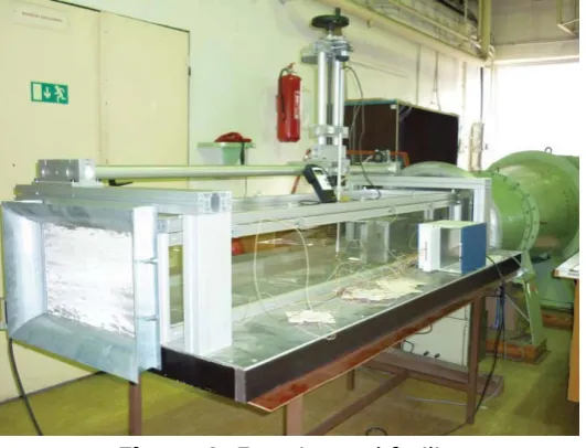
-coordinate for the three origin references he considered. Since the difference between both origins in the present investigation is not so large and has no a remarkable effect on the boundary layer parameters, it seems acceptable to consider the inlet of the test section as a reference point.The corresponding distances in the duct are shown in Table 1. Using the chosen origin, the boundary layers were found to be turbulent and the workable power-law formula had values of
n
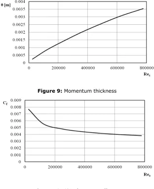
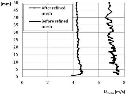
equal to 6. This suggestion fit in the experimental data obtained by HW with the theoretical calculation of the turbulent boundary layer. The main reason to represent the growth of the boundary layer with the help of the theory is the lack of information on the flow near the wall. The corresponding curve that shows this predicted growth of boundary-layer along the plate is represented in Figure 7. The parameters of the turbulent boundary layer over a flat plate at zero incidence such as displacement thickness, momentum thickness, friction coefficient and shape factor were calculated directly from Table 2 which provided by [16]. Figure 8 represents the velocity profile at four locations along the plate, specifically hole 3 to hole 6, while Figures 9 and 10 represent the momentum thickness,T
, and the skin friction coefficient,C
f , respectively.Figure 8: Velocity profile at different positions along the flat plate
Figure 9: Momentum thickness
4.2. Difficulties facing the experimental investigation
Although it is conventional to use a fabricated flat plate in the middle of a tunnel for conducting boundary layer experiments, it seems that it is possible to use the bottom wall of the tunnel for the same task under some restrictions and observations. The question rises here: do we always find the boundary layer which we are searching for? Since the boundary layer detected by the experimental investigation in this work is turbulent, it means that the test facility is failed to achieve the first rule mentioned by Saric [17] which describes the basic requirements for the boundary-layer stability experiments. The theoretical investigations of the boundary layers assume that the laminar flow is normally influenced by some disturbances which could come from different sources. Therefore, experiments are usually conducted in tunnel mainly under conditions of controlled disturbance excitation. This restriction implies that in the present study it is very important to maintain a satisfactory correlation of the experimental data with the stability theory to ensure that the basic state is probably correct.
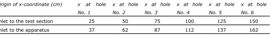
The main observed disturbance comes from the suction air source behind the apparatus. The affect of this disturbance on the average velocity profile variation in hole No. 1 located at 25 cm downstream of the leading edge is depicted in Figure 11. Reduction of influence of this source of disturbance on the mean flow has been done by inserting an additional fine mesh attached to the one which installed at the end of the tunnel. It is rather difficult to determine the exact boundary layer at this location since there is slight backflow up to approximately 3 mm over the plate. This result clarifies that additional sources of disturbances are exist.
It is well-known that turbulence may be initiated at the entrance of the duct or the pipe, therefore an exert effort was done to improve the entrance-flow geometry in such a way to reduce this effect. Since we used the bottom wall of the tunnel as a flat plate model, the laminar boundary layer expected to begin at the entrance with the same initial behaviour of the Blasius flat-plate solution but thinner than the Blasius estimate [18]. This fact is due to the retardation occurs near the wall which speeds up the potential core centre flow according to the requirements of the continuity state. Kandlikar S. G. and Campbell L. A. [12] verified that for severely disturbed entrance conditions a transitional flow may exist in the entire duct for specified range of Reynolds numbers, but in all cases it seems to be quite difficult in the present case to estimate that the non presence of the laminar boundary layer at the beginning of the plate is due to the effect of the rounded entrance used in the tunnel unless all other sources of disturbances are discover and solve or a new layout of the tunnel is establish and analyze.
ratios greater than 6. Acceptable location is somewhere between 0.38 and 0.45 unit span [17]. This true in all cases should never be in contradictory with the second rule of side-wall blockedge which implies that the disturbance amplitude near the side side-walls of the tunnel is different from linear theory. In the present experiment facility the measuring centre line is located at 0.4 of the width from the left side wall along the streamwise direction which clearly indicates that all holes after the third one located at 73 cm downstream from the leading edge are disturbed.
One of the main obstacles facing the measuring process is the wall proximity measurement. It is well-known that detailed information on the flow in the vicinity of the wall is of particular interest for viscous types of flow and heat transfer predictions [20]. The wall proximity corrections in some experiments are applied on the hot wire reading [21]. To be able to use the wall law to get information on the flow in the viscous sublayer this requires moving by hot wire very near to the wall and thereby the linear viscous relation could be implemented. In some experimental investigations they use microscope device to determine the last measuring point in the velocity profile while the lack of such device in the present work hampers efforts to accurately measure the distance between end of the profile and the wall. The near point to the wall was measured above 0.5 mm. The task of stability and transition experimentation is not an easy task. When designing new experiment equipment, many parameters characteristics must be taken into consideration. Some of these characteristics such as mesh sizes and locations, numbers of samples and background of pressure distribution in spanwise direction. Conducting such kind of these experiments reveals that the measurements characteristics require a special sensitivity to environmental conditions. When small change in an experimental set-up and measuring is done, this may introduce unanticipated disturbances which can complicate the flow details or skew the interpretation of the results.
Origin of x-coordinate (cm) x at hole
No. 1
x at hole
No. 2
x at hole
No. 3
x at hole
No. 4
x at hole
No. 5
x at hole
No. 6
Inlet to the test section 25 50 75 100 125 150
Inlet to the apparatus 37 62 87 112 137 162
Table 1: Optional of streamwise coordinate reference point
n
U u K1
G T G G* T G* H 5 1 Rex x
a G 5
1 Rex f C b 6 / 1
K 0.107143 0.142857 1.333333 0.337345906 0.057830727
Table 2: Turbulent boundary layer over flat plate at zero pressure gradient [16]
5. C
ONCLUSIONThe new designed apparatus is evaluated for transition experimentation by carrying out an experimental investigation for boundary layer flows over flat plate at approximately zero pressure gradient. In the range of freestream velocity from 3 to 8 m/s, only turbulent boundary layer is developed along the flat plate of the duct which means that the basic state in the test section is affected more or less by some disturbances. Main source of receptivity in the duct return to the air suction device located behind the duct, while the others sources of disturbances require more analysis. Since the investigation on this facility is still running, the present preliminary results give basic information on the flow behaviour through the duct and can be considered as database for coming improvement.
6. ACKNOWLEDGEMENTS
This work, which has been carried out at the Department of Mechanical Engineering at the University of Defence is supported by the Czech Science Foundation (project No. P101/10/0257) and by the research scheme of the Faculty of Military Technologies SV-K216.
7. R
EFERENCES[1] Surname1 A.B., Surname2 C.D.: Title, Published – where, Published – Who, Year, Pages (Style References)
[2] Reynolds O.: On the dynamical theory of turbulent incompressible viscous fluids and the determination of the criterion, Phil. Trans. R. Soc. London, 1884, A 186, pp. 123-161
[3] Rayleigh J. W. S.: On the stability or instability of certain fluid motions, Proc. London, Math. Soc. 9, 1880, pp. 57-70
[4] Heisenberg W.: Über Stabilität und Turbulenz von Flüssigkeits-strömmen, Ann. D. Physics. 1924, 74, pp. 577-627
[5] Tollmien W.: Über die Entstehung der Turbulenz Mitteilung, Math. Phys. Klasse-Göttingen, Nachr. Ges. Wiss., 1929, pp. 21-44
[7] Schlichting H.: Zur Entstehung der Turbulenz bei der Plattenströmung, Math. Phys. Klasse-Göttingen, Nachr. Ges. Wiss., 1933, pp. 181-208
[8] Schlichting H.: Amplitudenverteilung und Energiebilanz der kleinen Störungen bei der Plattenströmung, Math. Phys. Klasse, Fachgruppe I.-Göttingen, Nachr. Ges. Wiss, 1935, pp. 47-78
[9] Taylor G. I.: Statistical theory of turbulence, Effects of turbulence on boundary layer, Theoretical discussions of relationship between scale of turbulence and critical resistance of sphere, Proc. Roy. Soc. London, A 156(888), 1936, pp. 307-317
[10] Dryden H. L.: Boundary layer flow near at plates, Proc. Fourth International Congress for Appl. Mech. Cambridge 1934, p. 175
[11] Dryden H. L.: Airflow in the boundary layer near a plate, 1936, NACA TR 562 [12] Schubauer G. B., Skramstad H. K.: Laminar boundary layer oscillations and
transition on a flat plate, 1948, NACA TN 909
[13] Kandlikar S. G., Campbell L. A.: Effect of entrance condition on frictional losses and transition to turbulence, Proceedings of IMECE 2002, ASME International Mechanical Engineering Congress and Exposition, November 17-22, 2002, New Orleans, Louisana
[14] Fox R. W., McDonald A. T., Pritchard P.J.: Introduction to Fluid Mechanics, (7th
[15] Munson B. R., Young D. F., Okiishi T. H.: Fundamentals of Fluid Mechanics, (5th Edn), Hoboken: John Wiley and Sons, 2006, 562-590
Edn), New York: John Wiley and Sons, 2009, 389-411
[16] Kármán T. von: Über laminare und turbulente Reibung, Z. Angew. Math. Mech., 1921, Vol. 1, pp. 233-252 (English translation in NACA Technical Memo. 1092) [17] Libii J. N.: Laboratory exercises to study viscous boundary layers in the test
section of an open-circuit wind tunnel, World Transactions on Engineering and Technology Education, 2010, Vol.8, No.1
[18] Saric W. S.: Low-Speed Experiments: Requirements for Stability Measurements, AFOSR Contract No. F49620-85-C-0089 and NASA Grand NAG 805
[19] White F. M.: Viscous Fluid Flow, McGraw-Hill Companies, inc., 2006, ISBN 007-124493-X
[20] Becker S.: Personal communication, Fluid System Dynamics and Aeroacoustics, Institute of Process Technology and Systems Engineering, Cauerstr. 4, D-91058 Erlangen-Nuremberg, Germany, 2011
[21] Mitchell G., Chernoray V., Lofdahl L., Haasl S., Stemme G.: Measurements of the Turbulence Intensities in a Flat Plate Boundary Layer, Turbulence, Heat and Mass Transfer 4, @2003 Begell House, Inc., 2011
![Figure 7: Turbulent boundary layer development along the flat plate [� ]](https://thumb-us.123doks.com/thumbv2/123dok_us/8082598.1348703/8.595.144.449.465.608/figure-turbulent-boundary-layer-development-flat-plate.webp)