and Tweaking Discrete Pruning
Yoshinori Aono1, Phong Q. Nguyen2,3, and Yixin Shen4,3 1
National Institute of Information and Communications Technology, Japan 2 Inria Paris, France
3
CNRS, JFLI, University of Tokyo, Japan 4
IRIF, Univ Paris Diderot, CNRS, France
Abstract. Enumeration is a fundamental lattice algorithm. We show how to speed up enumeration on a quantum computer, which affects the security estimates of several lattice-based submissions to NIST: if T is the number of operations of enumeration, our quantum enumeration runs in roughly√T operations. This applies to the two most efficient forms of enumeration known in the extreme pruning setting: cylinder pruning but also discrete pruning introduced at Eurocrypt ’17. Our results are based on recent quantum tree algorithms by Montanaro and Ambainis-Kokainis. The discrete pruning case requires a crucial tweak: we modify the preprocessing so that the running time can be rigorously proved to be essentially optimal, which was the main open problem in discrete pruning. We also introduce another tweak to solve the more general problem of finding close lattice vectors.
1
Introduction
The main two hard lattice problems are finding short lattice vectors (SVP) and close lattice vectors (CVP), either exactly or approximately. Both have been widely used in cryptographic design for the past twenty years: Ajtai’s SIS [2] and Regev’s LWE [39] are randomized variants of respectively SVP and CVP.
With the NIST standardization of post-quantum cryptography and the devel-opment of fully-homomorphic encryption, there is a need for convincing security estimates for lattice-based cryptosystems. Yet, in the past ten years, there has been regular progress in the design of lattice algorithms, both in theory (e.g. [21,32,1]) and practice (e.g. [36,22,33,18,20,26,10]), which makes security esti-mates tricky. Lattice-based NIST submissions use varying cost models, which gives rise to a wide range of security estimates [5]. The biggest source of diver-gence is the cost assessment of a subroutine to find nearly shortest lattice vectors in certain dimensions (typically the blocksize of reduction algorithms), which is chosen among two families: sieving [3,36,33,26,14] and enumeration.
expense of missing solutions. One may only be interested in finding one point in
L∩S (provided it exists), or the ‘best’ point inL∩S,i.e.a point minimizing the distance to a target. Enumeration and cylinder pruning compute L∩S by a depth-first search of a tree with super-exponentially many nodes. Discrete pruning is different, but the computation ofS uses special enumerations.
The choice between sieving and enumeration for security estimates is not straightforward. On the one hand, sieving methods run in time 2O(n) much lower than enumeration’s 2O(nlogn), but require exponential space. On the other hand, until very recently [6], the largest lattice numerical challenges had all been solved by pruned enumeration, either directly or as a subroutine: cylinder prun-ing [22] for NTRU challenges [44] (solved by Ducas-Nguyen) and Darmstadt’s lattice challenges [29] (solved by Aono-Nguyen), and discrete pruning [20,10] for Darmstadt’s SVP challenges [40] (solved by Kashiwabara-Teruya). Among all lattice-based submissions [37,5] to NIST, the majority chose sieving over enumeration based on the analysis of NewHope [8, Sect. 6], which states that sieving is more efficient than enumeration in dimension≥250 for both classical and quantum computers. But this analysis is debatable: [8] estimates the cost of sieving by a lower bound (ignoring sub-exponential terms) and that of enumera-tion by an upper bound (either [18, Table 4] or [17, Table 5.2]), thereby ignoring the lower bound of [18] (see [11] for improved bounds).
The picture looks even more blurry when considering the impact of quantum computers, which is especially relevant to NIST standardization. The quantum speed-up is rather limited for sieving: the best quantum sieve algorithm runs in heuristic time 20.265n+o(n), only slighty less than the best classical (heuris-tic) time 20.292n+o(n) [26,14]. And the quantum speed-up for enumeration is unclear, as confirmed by recent discussions on the NIST mailing-list [4]. In 2015, Laarhovenet al. [27, Sect. 9.1] noticed that quantum search algorithms do not apply to enumeration: indeed, Grover’s algorithm assumes that the possible so-lutions in the search space can be indexed and that one can find thei-th possible solution efficiently, whereas lattice enumeration explores a search tree of an un-known structure which can only be explored locally. Three recent papers [8,19,7] mention in a short paragraph that Montanaro’s quantum backtracking algo-rithm [34] can speed up enumeration, by decreasing the number T of opera-tions to √T. However, no formal statement nor details are given in [8,19,7]. Furthermore, none of the lattice-based submissions to NIST cite Montanaro’s algorithm [34]: the only submission that mentions enumeration in a quantum setting is NTRU-HSS-KEM [24], where it is speculated that enumeration might have a√T quantum variant.
bases andtis the number of operations of a single enumeration) tom√tquantum operations, but we bring it down to√mt.
First, we clarify the application of Montanaro’s algorithm [34] to enumeration with cylinder pruning: the analysis of [34] assumes that the degree of the tree is bounded by a constant, which is tailored for constraint satisfaction problems, but is not the setting of lattice enumeration. To tackle enumeration, we add basic tools such as binary tree conversion and dichotomy: we obtain that if a lattice enumeration (with or without cylinder pruning) searches over a tree with
T nodes, the best solution can be found by a quantum algorithm using roughly √
T poly-time operations, where there is a polynomial overhead, which can be decreased if one is only interested in finding one solution. This formalizes earlier brief remarks of [8,19,7], and applies to both SVP and CVP.
Our main result is that the quantum quadratic speed-up also applies to the recent discrete pruning enumeration introduced by Aono and Nguyen [10] as a generalization of Schnorr’s sampling algorithm [41]. To do so, we tweak discrete pruning and use an additional quantum algorithm, namely that of Ambainis and Kokainis [9] from STOC ’17 to estimate the size of trees. Roughly speaking, given a parameterT, discrete pruning selectsT branches (optimizing a certain metric) in a larger tree, and derives T candidate short lattice vectors from them. Our quantum variant directly finds the best candidate in roughly√T operations.
As mentioned previously, we show that the quadratic speed-up of both enu-merations also applies to the extreme pruning setting (required to exploit the full power of pruning): if one runs cylinder pruning over m trees, a quantum enumeration can run in √T poly-time operations where T is the sum of them
numbers of nodes, rather than√mT naively; and there is a similar phenomenon for discrete pruning.
As a side result, we present two tweaks to discrete pruning [10], to make it more powerful and more efficient. The first tweak enables to solve CVP in such a way that most of the technical tools introduced in [10] can be reused. This works for the approximation form of CVP, but also its exact version for-malized by the Bounded Distance Decoding problem (BDD), which appears in many cryptographic applications such as LWE. In BDD, the input is a lattice basis and a lattice point shifted by some small noise whose distribution is cru-cial. We show how to handle the most important noise distributions, such as LWE’s Gaussian distribution and finite distributions used in GGH [23] and lat-tice attacks on DSA [35]. Enumeration, which was historically only described for SVP, can trivially be adapted to CVP, and so does [22]’s cylinder pruning [30]. However, discrete pruning [10] appears to be less simple.
time. But we also show that by a careful modification, the algorithm becomes provably efficient and even optimal for thatf, and heuristically for more general choices off: the running time becomes essentiallyT operations.
Our theoretical analysis has been validated by experiments, which show that in practical BDD situations, discrete pruning is as efficient as cylinder pruning. Since discrete pruning has interesting features (such as an easier parallelization and an easier generation of parameters), it might become the method of choice for large-scale blockwise lattice reduction.
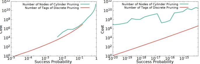
Impact. Fig. 1 illustrates the impact of our quantum enumeration on security estimates: the red and yellow curves show √#bases∗N where N is an upper bound cost, i.e., number of nodes of enumeration with extreme pruning with probability 1/#bases. The upper bounds for HKZ/Rankin bases are computed by the method of [11]. Here, we omitted the polynomial overhead factor because small factors in quantum sieve have also never been investigated. Note that the estimate 2(0.187βlogβ−1.019β+16.1)/2 (called Q-Enum in [5]) of a hypothetical quantum enumeration in NTRU-HSS-KEM [24], which is the square-root of a numerical interpolation of the upper bound of [18,17], is higher than our HKZ estimate: however, both are less than 2128until blocksize roughly 400.
Quantum enumeration with extreme pruning would be faster than quantum sieve up to higher dimensions than previously thought, around 300 if we assume that 1010 quasi-HKZ-bases can be obtained for a cost similar as enumeration, or beyond 400 if 1010 Rankin-bases (see [18]) can be used instead. Such ranges
Fig. 1. Q-sieve vs Q-enum: (Left) Using HKZ bases (Right) Using Rankin bases
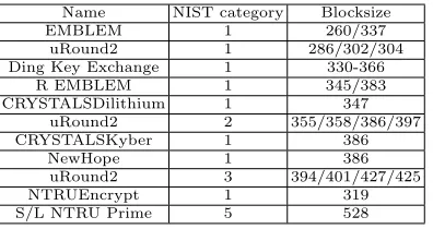
would affect the security estimates of between 11 and 17 NIST submissions (see Fig. 2), depending on which basis model is considered: these submissions state that the best attack runs BKZ with a blocksize seemingly lower than our threshold between quantum enumeration and quantum sieving, except in the case of S/L NTRU Prime, for which the blocksize 528 corresponds to less than 2200in Fig. 1, whereas the target NIST category is 5.
Furthermore, we note that our quantum speedup might actually be more than quadratic. Indeed, the numberT of enumeration nodes is actually a ran-dom variable: the average quantum running time is E(√T), which is≤p
E(T)
Name NIST category Blocksize
EMBLEM 1 260/337
uRound2 1 286/302/304
Ding Key Exchange 1 330-366
R EMBLEM 1 345/383
CRYSTALSDilithium 1 347
uRound2 2 355/358/386/397
CRYSTALSKyber 1 386
NewHope 1 386
uRound2 3 394/401/427/425
NTRUEncrypt 1 319
S/L NTRU Prime 5 528
Fig. 2. Lattice-based NIST submissions affected by quantum enumeration
to identify the distribution of T: it cannot be log-normal for LLL bases (un-like what seems to be suggested in [45]), because it would violate the provable running time 2O(n2)
of enumeration with LLL bases.
On the other hand, we stress that this is just a first assessment of quantum enumeration. If one is interested in more precise estimates, such as the number of quantum gates, one would need to assess the quantum cost of the algorithm of Montanaro [34] and that of Ambainis and Kokainis [9].
Related work. Babai’s nearest plane algorithm [13] can be viewed as the first form of BDD discrete pruning, using only a single cell. Lindner-Peikert’s algo-rithm [28] generalizes it using exponentially many cells, and is the BDD analogue of Schnorr’s random sampling [41] (see [30]). But for both [41,28], the selection of cells is far from being optimal. In 2003, Ludwig [31] applied Grover search to speed up [41] quantumly.
Roadmap. Sect. 2 provides background. Sect. 3 gives a general description of enumeration to find close lattice vectors. In Sect. 4, we speed up cylinder pruning enumeration on a quantum computer, using [34]. In Sect. 5, we adapt lattice enumeration with discrete pruning to CVP. In Sect. 6, we show how to efficiently select the best parameters for discrete pruning, by modifying the orthogonal enumeration of [10]. In Sect. 7, we speed up discrete pruning enumeration on a quantum computer, using [34,9]. Supplementary material is given in Appendix, including proofs and experimental results.
2
Preliminaries
We follow the notations of [10].
General. Nis the set of integers≥0. For any finite setU, its number of elements
is #U. For any measurable subset S ⊆Rn, its volume is vol(S). We use row
representations of matrices. The Euclidean norm of a vector v∈Rn iskvk. We
denote by Balln(c, R) then-dim Euclidean ball of radiusRand centerc, whose volume is vol(Balln(R)) =Rn π
n/2
Lattices. A lattice L is a discrete subgroup of Rm, or equivalently the set
L(b1, . . . ,bn) ={ Pn
i=1xibi : xi∈Z} of all integer combinations of nlinearly
independent vectorsb1, . . . ,bn ∈Rm. Suchbi’s form abasis ofL. All the bases have the same number n of elements, called the dimension or rank of L, and the same n-dimensional volume of the parallelepiped {Pni=1aibi : ai∈[0,1)} they generate. We call this volume the co-volume ofL, denoted by covol(L). The latticeLis said to befull-rankifn=m. Theshortest vector problem(SVP) asks to find a non-zero lattice vector of minimal Euclidean norm. Theclosest vector problem(CVP) asks to find a lattice vector closest to a target vector.
Orthogonalization. For a basisB = (b1, . . . ,bn) of a latticeLandi∈ {1, . . . , n}, we denote by πi the orthogonal projection on span(b1, . . . ,bi−1)⊥. The Gram-Schmidt orthogonalization of the basisBis defined as the sequence of orthogonal vectors B? = (b?
1, . . . ,b?n), where b?i := πi(bi). We can write each bi as b?i + Pi−1
j=1µi,jb?j for some unique µi,1, . . . , µi,i−1 ∈ R. Thus, we may represent the
µi,j’s by a lower-triangular matrixµwith unit diagonal.πi(L) is a lattice of rank
n+ 1−igenerated byπi(bi), . . . , πi(bn), with covol(πi(L)) = Qn
j=i b?j.
Gaussian Heuristic. The classical Gaussian Heuristic provides an estimate on the number of lattice points inside a “nice enough” set:
Heuristic 1 Given a full-rank latticeL⊆Rn and a measurable setS⊆Rn, the
number of points inS∩Lis approximately vol(S)/covol(L).
Both rigorous results and counter-examples are known (see [10]). One should therefore experimentally verify its use, especially for pruned enumeration which relies on strong versions of the heuristic, where the setS is not fixed, depending on a basis ofL.
Statistics. We denote byE() the expectation andV() the variance of a random
variable. For discrete pruning, it is convenient to extendE() to any measurable
setC ofRn by using the squared norm, that isE{C}:=Ex∈C(kxk2).
Gaussian distribution. The CDF of the Gaussian distribution of expectation 0 and variance σ2 is 1
2(1 + erf( x
σ√2)) where the error function is erf(z) := 2
√ π
Rz 0 e
−t2
dt. The multivariate Gaussian distribution over Rm of parameter σ selects each coordinate with Gaussian distribution.
Quantum Tree Algorithms. Like in [9], a treeT is locally accessed given: 1. the rootrofT
2. a black box which, given a node v, returns the number of childrend(v) for this node. Ifd(v) = 0, vis called a leaf.
We denote by V(T) its set of nodes, L(T) its set of leaves, d(T) = maxv∈V(T)d(v) its degree andn(T) an upper-bound of its depth. When there is no ambiguity, we usedandndirectly without the argumentT. We also denote by #T the number of nodes of the treeT.
Backtracking is a classical algorithm for solving problems such as constraint satisfaction problems, by performing a tree search in depth-first order. Each node represents a partial candidate and its children say how to extend a candidate. There is a black-box function P : V(T) → {true, f alse, indeterminate} such that P(v) ∈ {true, f alse} iff v is a leaf: a node v ∈ V(T) is called marked if P(v) = true. Backtracking determines whetherT contains a marked node, or outputs one or all marked nodes. Classically, this can be done in #V(T) queries. Montanaro [34] studied the quantum case:
Theorem 2 ([34]). There is a quantum algorithm
ExistSolution(T, T,P, n, ε)which givenε >0, a treeT such thatd(T) =O(1), a black box function P, and upper bounds T andn on the size and the depth of T, determines ifT contains a marked node by makingO(√T nlog(1/ε))queries to T and to the black box function P, with a probability of correct answer ≥1−ε. It usesO(1)auxiliary operations per query and uses poly(n)qubits.
Theorem 3 ([34]). There is a quantum algorithm FindSolution(T,P, n, ε) which, givenε >0, a treeT such thatd(T) =O(1), a black box functionP, and an upper bound non the depth of T, outputsxsuch that P(x)is true, or “not found” if no suchxexists by makingO(p#V(T)n3/2log(n) log(1/ε))queries to T and to the black box functionP, with correctness probability at least 1−ε. It uses O(1) auxiliary operations per query and usespoly(n)qubits.
Notice that Th. 3 does not require an upper-bound on #V(T) as input. Ambainis and Kokainis [9] gave a quantum algorithm to estimate the size of trees, with input a treeT and a candidate upper boundT0 on #V(T). The algorithm must output an estimate for #V(T),i.e.either a number of ˆT ∈[T0] or a claim “T contains more thanT0vertices”. The estimate is δ-correct if:
1. the estimate is ˆT ∈[T0] which satisfies|T−Tˆ| ≤ δT whereT is the actual number of vertices;
2. the estimate is “T contains more thanT0 vertices” and the actual number of verticesT satisfies (1 +δ)T > T0.
An algorithm solves the tree size estimation problem up to precision 1±δwith correctness probability at least 1−ε if for any T and any T0, the probability that it outputs aδ-correct estimate is at least 1−ε.
Theorem 4 ([9]). There is a quantum algorithm
TreeSizeEstimation(T, T0, δ, ε) which, given ε > 0, a tree T, and upper bounds d and n on the degree and the depth of T, solves tree size estimation up to precision 1 ±δ, with correctness probability at least 1 −ε. It makes
O
√ nT0
δ1.5 dlog
2
3
Enumeration with Pruning
We give an overview of lattice enumeration and pruning, for the case of finding close lattice vectors, rather than finding short lattice vectors: this revisits the analysis model of both [22] and [10].
3.1 Finding Close Vectors by Enumeration
Let L be a full-rank lattice in Rn. Given a target u ∈ Qn, a basis B =
(b1, . . . ,bn) ofLand a radiusR >0, enumeration [38,25] outputsL∩S where
S= Balln(u, R): by comparing all the distances tou, one extracts a lattice vec-tor closest tou. It performs a recursive search using projections, to reduce the dimension of the lattice: ifkvk ≤R, thenkπk(v)k ≤Rfor all 1≤k≤n. One can easily enumerateπn(L)∩S. And if one enumeratesπk+1(L)∩Sfor somek≥1, one can deriveπk(L)∩S by enumerating the intersection of a one-dimensional lattice with a suitable ball, for each point inπk+1(L)∩S. Concretely, it can be viewed as a depth-first search of the enumeration treeT which is a target of the quantum speed-up: the nodes at depthn+ 1−kare the points ofπk(L)∩S. The classical/quantum running-times of enumeration depends on Rand the quality ofB, but is typically super-exponential inn, even ifL∩S is small.
3.2 Finding Close Vectors by Enumeration with Pruning
We adapt the general form of enumeration with pruning introduced by [10]: pruned enumeration uses a pruning set P ⊆Rn, and outputsL∩(u+P). The
advantage is that for suitable choices of P, enumerating L∩(u+P) is much cheaper than L∩S, and if we further intersect L∩(u+P) with S, we may have found non-trivial points ofL∩S. Note that we use u+P rather thanP, because it is natural to makeP independent ofu, and it is what happens when one uses the pruning of [22] to search for close vectors. Following [22], we view the pruning setP as a random variable: it depends on the choice of basisB.
We distinguish two cases, which were considered separately in [10,22]:
Approximation setting: This was studied in [10], but not in [22]. Here, we are interested in finding any point inL∩S∩(u+P) by enumeratingL∩(u+P) then intersect it with the ballS, so we define the success probability as:
Pr
succ= PrP,u(L∩S∩(u+P)6=∅), (1)
which is the probability that it outputs at least one point in L∩S. By (slightly) adapting the reasoning of [10] based on the Gaussian heuristic, we estimate that (1) is heuristically
Pr
succ≈min(1,vol(S∩(u+P))/covol(L)), (2) and that the number of elements ofL∩S∩(u+P) is roughly vol(S∩(u+
Unique setting: Here, we know that the target u is unusually close to the lattice, that isL∩S is a singleton, and we want to find the closest lattice point tou: this is the so-calledBounded Distance Decodingproblem (BDD), whose hardness is used in most lattice-based encryption schemes. Thus,uis of the formu=v+e wherev ∈L ande∈Rn is very short, and we want
to recoverv. This was implicitly studied in [22], but not in [10]: [22] studied the exact SVP case, where one wants to recover a shortest lattice vector (in our setting, if the targetu∈L, the BDD solution would beu, but one could alternatively ask for the closest distinct lattice point, which can be reduced to finding a shortest lattice vector). We are only interested in finding the closest lattice pointv∈L, so we define the success probability as:
Pr
succ= PrP,u(v∈L∩(u+P)), (3)
because we are considering the probability that the solutionvbelongs to the enumerated setL∩(u+P). Usually, the targetuis derived from the noise e, which has a known distribution, then we can rewrite (3) as:
Pr
succ= PrP,e(0∈e+P) = PrP,e(−e∈P). (4)
In the context of SVP, we would instead define Prsucc= PrP(v∈P) wherev is a shortest lattice vector. In general, it is always possible to makeudepend solely one: one can take a canonical basis ofL, like the HNF, and use it to reduceumoduloL, which only depends one. Whether PrP,e(−e∈P) can
be evaluated depends on the choice ofP and the distribution of the noisee. For instance, if the distribution of−e is uniform over some measurable set
E, then:
Pr
P,e(−e∈P) =
vol(E∩P) vol(E) .
We discuss other settings in Sect. 5.6. This can be adapted to a discrete distribution. If the distribution of−e is uniform over a finite set E∩Zn,
then:
Pr
P,e(−e∈P) =
#(E∩P∩Zn)
#(E∩Zn)
,
where #(E∩P∩Zn) is heuristically≈vol(E∩P) by the Gaussian heuristic, and #(E∩Zn) is usually given by the specific choice ofE.
When it fails, we can simply repeat the process with many differentP’s until we solve the problem, in the approximation-setting or the unique-setting.
We have discussed ways to estimate the success probability of pruned enu-meration. To estimate the running time of the full algorithm, we need more information, which depends on the choice of pruning:
– An estimate of the cost of enumeratingL∩S∩(u+P).
3.3 Cylinder Pruning
The first pruning setP ever used is the following generalization [22] of pruned enumeration of [42,43]. There,P is defined by a functionf :{1, . . . , n} →[0,1], a radius R >0 and a lattice basisB = (b1, . . . ,bn) as follows:
Pf(B, R) ={x∈Rn s.t.kπn+1−i(x)k ≤f(i)R for all 1≤i≤n}, (5) where theπi’s are the Gram-Schmidt projections defined byB. We callcylinder pruning this form of enumeration, becausePf(B, R) is an intersection of cylin-ders: each inequalitykπn+1−i(x)k ≤f(i)R defines a cylinder. Cylinder pruning was introduced in the SVP setting, but its adaptation to CVP is straightfor-ward [30].
Gama et al. [22] showed how to efficiently compute tight lower and upper bounds for vol(Pf(B, R)), thanks to the Dirichlet distribution and special inte-grals. Then we can do the same for vol(Pf(B, R)∩S) ifS is any zero-centered ball. Using the shape ofPf(B, R), [22] also estimated of the cost of enumerating
L∩S∩Pf(B, R), using the Gaussian heuristic on projected latticesπi(L): these estimates are usually accurate in practice, and they can also be used in the CVP case [30]. To optimize the whole selection of parameters, one finally needs to take into account the cost of computing the (random) reduced basisB: for instance, this is done in [18,12].
4
Quantum speed-up of Cylinder Pruning
4.1 Tools
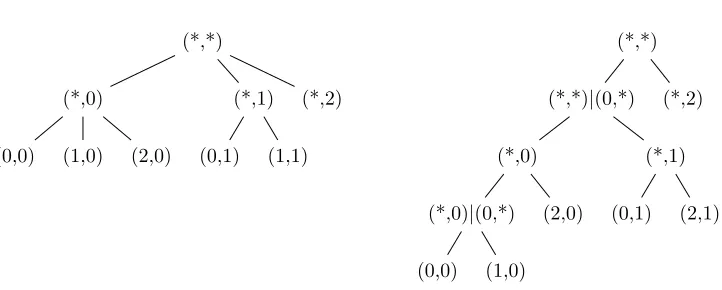
The analysis of quantum tree algorithms requires the tree to have constant de-greed=O(1). Without this assumption, there is an extrapoly(d) term in the complexity bound like in Th. 4. Instead, it is more efficient to first convert the tree into a binary tree, so that the overhead is limited to poly(logd). We will use the following conversion (illustrated by Fig. 3):
Theorem 5. One can transform any tree T of depth n and degree d into a binary one T2 so that: T2 can be explored locally; T and T2 have roughly the same number of nodes, namely#T ≤#T2≤2#T; the leaves ofT andT2 are identical; the depth of T2 is ≤ nlogd. Moreover, a black-box function P over T can be adapted a black box P2 forT2, so that the marked nodes of T andT2 are the same. One query to P2 requires at most one query to P with additional
O(logd) auxiliary operations.
In the context of enumeration with pruning, instead of enumerating the whole set L∩S, we may only be interested in the ‘best’ vector in L∩S, i.e. which minimize some distance. In terms of tree, this means that given a tree T with marked leafs defined by a predicateP, we want to find a marked leaf minimizing an integral functiongwhich is defined on the marked leaves ofT. We know that
(*,*)
(*,0)
(0,0) (1,0) (2,0)
(*,1)
(0,1) (1,1) (*,2)
(*,*)
(*,*)|(0,*)
(*,0)
(*,0)|(0,*)
(0,0) (1,0) (2,0)
(*,1)
(0,1) (2,1) (*,2)
Fig. 3. An example of the transformation in Th. 5
gV the predicate which returns true on a nodeN if and only if it is a marked leaf andg(N)≤V. We first find a parameterRsuch that there is at least one marked leafN such thatg(N)≤R. Then we decreaseRby dichotomy using Th. 3 with different marking functions. We thus obtainFindMin1(T,P, g, R, d, ε) (Alg. 1), which is a general algorithm to find a leaf minimizing the functiong with error probability ε, using the binary treeT2.
Algorithm 1Finding a minimum:FindMin1(T,P, g, R, d, ε)
Input: A tree T with marked leaves defined by the predicate P. An integral function g defined on the marked leaves of T. A parameter R, such that
g(N)≤Rhas at least one solution over all of the marked leaves. An upper-bounddof the number of children of a node in T.
Output: A marked leaf N such thatg takes its minimum onN among all the marked leaves explored by the backtracking algorithm.
1: T2←the corresponding binary tree ofT.5
2: N←R,N0←0,Round← dlog2Re,v←(0,· · ·,0) 3: whileN0< N−1do
4: CallFindSolution(T2, gb(N+N0)/2e, nlogd, ε/Round)
5: if FindSolution(T2, gb(N+N0)/2e, nlogd, ε/Round) returnsx then 6: v←x,N ← b(N+N0)/2e
7: else
8: N0← b(N+N0)/2e 9: end if
10: end while
11: return v
5
Theorem 6. Let ε > 0. Let T be a tree with its marked leaves defined by a predicate P. Let d be an upper-bound on the degree of T. Let g be an integral function defined on the marked leaves such that g(N) ≤ R has at least one solution over all of the marked leaves. Then Alg. 1 outputs N ∈ T such thatg
takes its minimum on N among all of the marked leaves ofT, with probability at least 1−ε. It requires O(√T(nlogd)3/2log(nlogd) log(dlog
2Re/ε)dlog2Re) queries on T and on P, where T = #T. Each query on T requires O(logd) auxiliary operations. The algorithm needs poly(nlogd,logR)qubits.
Proof. Correctness is trivial. Regarding the query complexity, there are in total Round = dlog2Re calls to FindSolution. According to Th. 3, each call requires O(√T(nlogd)3/2log(nlogd) log(Round/ε)) queries on the local structure of T2 and on g. Thus according to Th. 5, in total, we need
O(√T(nlogd)3/2log(nlogd) log(dlog
2Re/ε)dlog2Re) queries on the local struc-ture of T and on g. Each query on T requires O(logd) auxiliary operations. For each call, we needpoly(nlogd) qubits. In total, we needpoly(nlogd,logR)
qubits. ut
If we know an upper-bound of T of the number of nodes in the tree T, we can speed up the algorithm by replacing FindSolution by ExistSolution
in lines 4, 5: the new algorithm is given and analyzed in Appendix as Alg. 8 (FindMin2(T,P, g, R, d, T, ε)).
4.2 Application to Cylinder Pruning
Lemma 1. Let(b1,· · · ,bn)be an LLL-reduced basis. LetT be the backtracking tree corresponding to the cylinder pruning algorithm for SVP with radius R ≤ kb1k and bounding function f. Then the degree of the tree satisfies:d(T)≤2n. Proof. In T, the number of children of a node N of depth k can be upper-bounded by dk = 2f(k) k
b1k
kb? n−k+1k
+ 1≤2(n−k)/2+1+ 1. The result follows from the fact that an LLL-reduced basis satisfies: kb1k2
kb? ik2 ≤2
i−1 for all 1≤i≤n. ut
Theorem 7. There is a quantum algorithm which, givenε >0, an LLL-reduced basisB = (b1,· · ·,bn)of a lattice L in Zn, a radius R≤ kb1k and a bounding
function f :{1,· · ·, n} →[0,1], outputs with correctness probability≥1−ε: 1. a non-zero vector v in L ∩ Pf(B, R), in time
O(√T n3poly(log(n),log(1/ε)))), if L∩P
f(B, R)6⊆ {0}.
2. all vectors in L ∩ Pf(B, R), in time O(#(L ∩
Pf(B, R)) √
T n3log(n)poly(log(#(L∩P
f(B, R)),log(1/ε))).
3. a shortest non-zero vector v in L ∩ Pf(B, R), in time
O(√T n3β
poly(log(n),log(1/ε),log(β))), if L ∩ Pf(B, R) 6⊆ {0}. Here
β is the bitsize of the vectors of B.
Proof. Let T be the enumeration tree searched by the cylinder pruning al-gorithm in which a node of depth i, where 1 ≤ i ≤ n, is encoded as (∗,· · ·,∗, xn−i+1,· · · ,· · · , xn) and where the root is encoded as (∗,· · ·,∗). LetT2 be the corresponding binary tree. LetPbe a predicate which returns true only on the nodes encoded as (x1,· · ·, xn) inT2(i.e.the leaves ofT2, where all the vari-ables are assigned), such thatkPni=1xibik2≤R2and (x
1,· · ·, xn)6= (0,· · · ,0). For 1, if L∩Pf(B, R) 6= ∅, we apply FindSolution(T2,P, nlogd, ε). For 2, we find all marked nodes by simply repeating the algorithm FindSolution, modifying the oracle operator to strike out previously seen marked elements, which requires space complexityO(#(L∩Pf(B, R))).
For 3, if L ∩ Pf(B, R) 6= ∅, we apply Th. 6 to FindMin1(T,P,k · k2, R2,2n + 1, ε). In T
2, the height of the tree can be upper-bounded by
nlogd = O(n2). We also have Round = O(β). The time complexity is
O(√T n3βpoly(log(n),log(1/ε),log(β))). ut As corollary, we obtain the following quantum speed-up of Kannan’s algo-rithm for the shortest vector problem:
Theorem 8. There is a quantum algorithm which, givenε >0, and a basis B
of a full-rank lattice L in Zn, with entries of bitlength≤ β, outputs a shortest
non-zero vector of L, with error probability at most ε, in time (n4ne +o(n))·
poly(log(n),log(1/ε), β)usingpoly(n, β)qubits.
We can also apply the quantum tree algorithms to extreme pruning. If we run cylinder pruning overmtrees, we can combine these trees into a global one and apply the quantum tree algorithms on it.
Theorem 9 (Quantum speed-up for SVP extreme pruning). There is
a quantum algorithm which, given ε > 0, m LLL-reduced bases B1,· · ·Bm of a lattice L in Zn,a radius R ≤ min
ikb1,ik where b1,i is the first vector of
Bi and a bounding function f : {1,· · ·, n} → [0,1], outputs with correctness probability ≥ 1−ε a shortest non-zero vector v in L∩(∪Pf(Bi, R)), in time
O(√T n3βpoly(log(n),log(1/ε),log(β),log(m))), ifL∩(∪Pf(Bi, R)6⊆ {0}. Here
β is a bound on the bitsize of vectors of Bi’s, T is the sum of number of nodes in the enumeration trees Ti searched by cylinder pruning over Pf(Bi, R) for all 1≤i≤m.
In the case of CVP with target vector u, we use the cylinder pruning al-gorithm with radius R ≤ pPni=1kb?
ik2/2 and bounding function f. The de-gree of the tree is now upper-bounded by d = maxpPni=1kb?
ik2/kb?jk + 1. We have logd = O(β +n) where β is the bitsize of the vectors of the ba-sis B. We can obtain a similar theorem as Th. 7 with different overheads. For exemple for the first case, the time complexity becomes O(√T n3/2(n+
β)3/2poly(log(n),log(1/ε),log(β)))).
For the extreme pruning for CVP the time complexity is O(√T n3/2(n+
5
BDD Enumeration with Discrete Pruning
We adapt Aono-Nguyen’s discrete pruning [10] to the BDD case. First, we recall discrete pruning, then we modify it.
5.1 Discrete Pruning for the Enumeration of Short Vectors
Discrete pruning is based on lattice partitions defined as follows. Let L be a full-rank lattice inQn. AnL-partition is a partition CofRn such that:
– The partition is countable:Rn =∪
t∈TC(t) where T is a countable set, and C(t)∩ C(t0) =∅whenevert6=t0.
– Each cellC(t) contains a single lattice point, which can be found efficiently: given any t ∈ T, one can “open” the cell C(t), i.e. compute C(t)∩L in polynomial time. In other words, the partition defines a functiong:T →L
whereC(t)∩L={g(t)}, and one can computeg in polynomial time. Discrete pruning is obtained by selecting the pruning set P as the union of finitely many cells C(t), namely P = ∪t∈UC(t) for some finite U ⊆ T. Then
L∩P =∪t∈U(L∩ C(t)) can be enumerated by opening each cell C(t) fort∈U. [10] presented two usefulL-partitions: Babai’s partition where T =Zn and each cell C(t) is a box of volume covol(L); and the natural partition where
T =Nn and each cell C(t) is a union of non-overlapping boxes, with total vol-ume covol(L). The natural partition is preferable, and [10] explained how to select good cells for the natural partition. In theory, one would like to select the cellsC(t) which maximize vol(C(t)∩S): [10] shows how to compute vol(C(t)∩S), but an exhaustive search to derive the best vol(C(t)∩S) exactly would be too expensive. Instead, [10] shows how to approximate efficiently the optimal selec-tion, by selecting the cells C(t) minimizing E(C(t)): given m, it is possible to
compute in practice them cells which minimizeE(C(t)).
5.2 Universal Lattice Partitions
Unfortunately, in the worst case, L-partitions are not sufficient for our frame-work: if P = ∪t∈UC(t), then L∩(P +u) = ∪t∈U(L∩(C(t) +u)) but the number of elements in L∩(C(t) +u) is unclear, and it is also unclear how to compute in L∩(C(t) +u) efficiently. To fix this, we could compute instead
L∩P∩S=∪t∈U(L∩ C(t))∩S, but that creates two issues:
– In the unique setting, it is unclear how we would evaluate success probabil-ities. Given a tagtand a targetu=v+e wheree is the noise andv∈L, we would need to estimate the probability thatv∈ C(t),i.e.u−e∈ C(t).
– We would need to select the tag setU depending on the targetu, without knowing how to evaluate success probabilities.
Definition 1. Let L be a full-rank lattice inQn. An L-partition C is universal if for all u∈Qn, the shifted partitionC+u is anL-partition,i.e.:
– The partition is countable:Rn =∪t∈TC(t) where T is a countable set, and C(t)∩ C(t0) =∅ whenevert6=t0.
– For anyu∈Qn, each cellC(t)contains a single point inL−u={v−u,v∈
L}, which can be found efficiently: given any t ∈ T and u ∈ Qn, one can
“open” the cellu+C(t),i.e. compute(u+C(t))∩Lin polynomial time. Unfortunately, an L-partition is not necessarily universal, even in dimension one. Indeed, consider the L-partition C with T =Zdefined as follows: C(0) =
[−1/2,1/2]; For any k >0, C(k) = (k−1/2, k+ 1/2]; For any k <0, C(k) = [k−1/2, k+ 1/2). It can be checked that C is not universal: the shifted cell C(0)+1/2 contains two lattice points, namely 0 and 1. Fortunately, we show that the two L-partitions (related to Gram-Schmidt orthogonalization) introduced in [10] for discrete pruning are actually universal:
Lemma 2. Let B be a basis of a full-rank latticeL inZn. Let T =Zn and for
any t ∈ T,CZ(t) = tB?+D where D = {Pni=1xib?i s.t. −1/2 ≤xi <1/2}. Then Babai’s L-partition(CZ(), T)with Alg. 9 (in App.) is universal.
Lemma 3. Let B be a basis of a full-rank lattice L in Zn. Let T = Nn and
for any t = (t1, . . . , tn) ∈ T, CN(t) = {
Pn
i=1xib?i s.t. −(ti + 1)/2 < xi ≤ −ti/2orti/2 < xi ≤ (ti + 1)/2}. Then the natural partition (CN(), T) with
Alg. 10 (in App.) is universal.
5.3 BDD Discrete Pruning from Universal Lattice Partitions
Any universalL-partition (C, T) and any vectoru∈Qn define a partitionRn=
∪t∈T(u+C(t)). Following the SVP case, discrete pruning opens finitely many cellsu+C(t), as done by Alg. 2: discrete pruning is parametrized by a finite set
U ⊆T of tags, specifying which cellsu+C(t) to open. It is therefore a pruned CVP enumeration with pruning setP =∪t∈UC(t).
Algorithm 2Close-Vector Discrete Pruning from Universal Lattice Partitions
Input: A target vector u ∈ Qn, a universal lattice partition (C(), T), a finite
subsetU ⊆T and if we are in the approximation setting, a radiusR.
Output: L∩(u+ (S∩P)) whereS= Balln(R) andP =∪t∈UC(t). 1: R=∅
2: fort∈U do
3: ComputeL∩(u+C(t)) by openingu+C(t): in the approx setting, check if the output vector is within distance ≤R to u, then add the vector to the setR. In the unique setting, check if the output vector is the solution. 4: end for
The algorithm performs exactlykcell openings, wherek= #U is the number of cells, and each cell opening runs in polynomial time. So the running time is #U poly-time operations: one can decide how much time should be spent.
Since the running time is easy to evaluate like in the SVP case, there are only two issues: how to estimate the success probability and how to select U
(which defines the pruning setP =∪t∈UC(t)), in order to maximize the success probability.
5.4 Success Probability
Following Sect. 3.2, we distinguish two cases:
Approximation setting: Based on (2), the success probability can be derived from:
vol(S∩(u+P)) =X
t∈U
vol(Balln(R)∩ C(t)). (6)
This is exactly the same situation as in the SVP case already tackled by [10]. They showed how to compute vol(Balln(R)∩ C(t)) for Babai’s partition and the natural partition by focusing on the intersection of a ball with a box
H={(x1, . . . , xn)∈Rn s.t.αi≤xi≤βi}:
– In the case of Babai’s partition, each cellCZ(t) is a box.
– In the case of the natural partition, each cell CN(t) is the union of 2j symmetric (non-overlapping) boxes, where j is the number of non-zero coefficients of t. It follows that vol(CN(t)∩Balln(R)) = 2jvol(H ∩S),
whereH is any of these 2j boxes.
And they also showed to approximate a sumP
t∈Uvol(Balln(R)∩ C(t)) in practice, without having to compute separately each volume.
Unique setting: Based on (4), if the noise vector ise, then the success prob-ability is
Pr
succ= PrP,e(−e∈P) =
X
t∈U Pr
P,e(−e∈ C(t)) (7)
It therefore suffices to compute the cell probability PrP,e(e∈ C(t)), instead
of an intersection volume. Similarly to the approximation setting, we might be able to approximate the sumP
t∈UPrP,e(e ∈ C(t)) without having to
compute individually each probability. In Sect. 5.6, we focus on the natural partition: we discuss ways to compute the cell probability PrP,e(e ∈ C(t))
depending on the distribution of the noisee.
In both cases, we see that the success probability is of the form: Pr
succ= X
t∈U
f(t), (8)
for some functionf() :T →[0,1] such thatP
due to the Gaussian heuristic. If ever the computation of f() is too slow to compute individually each term ofP
t∈Uf(t), we can use the statistical inference techniques of [10] to approximate (8) from the computation of a small number of
f(t). Note that if we know that the probability is reasonably large, say>0.01, we can alternatively use Monte-Carlo sampling to approximate it.
5.5 Selecting Parameters
We would like to select the finite setU of tags to maximize Prsucc given by (8). Let us assume that we have a function g : T →R+ such that Pt∈Tg(t) con-verges. If (8) provably holds, thenP
t∈Tf(t) = 1, so the sum indeed converges. SinceT is infinite, this implies that for anyB >0, the set{t∈T s.t.f(t)> B} is finite, which proves the following elementary result:
Lemma 4. Let T be an infinite countable set. Let f : T → R+ be a function such that P
t∈Tf(t) converges. Then for any integer m > 0, there is a finite subset U ⊆ T of cardinal m such that f(t) ≤minu∈Uf(u) for all t ∈ T \U. Such a subset U maximizes P
u∈Uf(u)among all m-size subsets ofT.
Any such subsetU would maximize Prsuccamong allm-size subsets ofT, so we would ideally want to select such a U for any given m. And m quantifies the effort we want to spend on discrete pruning, since the bit-complexity of discrete pruning is exactlympoly-time operations.
Now that we know that optimal subsetsU exist, we discuss how to find such subsetsU efficiently. In the approximation setting of [10], the actual functionf() is related to volumes: we want to select thekcells which maximize vol(Balln(R)∩ C(t)) among all the cells. This is too expensive to do exactly, but [10] provides a fast heuristic method for the natural partition, by selecting the cells C(t) minimizing E{CN(t)}: given as inputm, it is possible to compute efficiently in
practice the tags of themcells which minimize
E{CN(t)}=
n X
i=1 t2
i 4 +
ti 4 +
1 12
kb?ik2.
In other words, this is the same as replacing the functionf() related to volumes by the function
h(t) =e−
Pn i=1
t2i
4+
ti
4+ 1 12
kb?ik2
,
and it can be verified thatP
t∈Nnh(t) converges. In practice (see [10]), the m
cells maximizingh(t) (i.e.minimizingE{CN(t)}) are almost the same as the cells
maximizing vol(Balln(R)∩ C(t)).
5.6 Noise Distributions in the Unique Setting
We discuss how to evaluate the success probability of BDD discrete pruning in the unique setting for the natural partition. This can easily be adapted to Babai’s partition, because it also relies on boxes. Following (7), it suffices to evaluate:
p(t) = Pr
P,e(e∈ −C(t)), (9)
whereP is the (random) pruning set,eis the BDD noise andC(t) is the cell of the tag t. We now analyze the most frequent distributions fore.
LWE and Gaussian Noise. The most important BDD case is LWE [39]. How-ever, there are many variants of LWE using different distributions of the noise e. We will use the continuous Gaussian distribution overRn, like in [39]. Many
schemes actually use a discrete distribution, such as some discrete Gaussian dis-tribution over Zn (or something easier to implement): because this is harder to
analyze, cryptanalysis papers such as [28,30] prefer to ignore this difference, and perform experiments to check if it matches with the theoretical analysis. The main benefit of the Gaussian distribution over Rn is that for any basis, each
coordinate is a one-dimensional Gaussian.
Lemma 5. Let t = (t1, . . . , tn) ∈ Nn be a tag of the natural partition CN()
with basis B = (b1, . . . ,bn). If the noise e follows the multivariate Gaussian distribution overRn with parameter σ, then:
p(t) = n Y
i=1
erf
1 √
2σ· ti+ 1
2 · kb ? ik
−erf
1 √
2σ· ti 2 · kb
? ik
(10)
Spherical Noise. If the noise e is uniformly distributed over a centered ball, we can reuse the analysis of [10]:
Lemma 6. Let(C, T)be a universalL-partition. Lett∈T be a tag. If the noise eis uniformly distributed over then-dimensional centered ball of radiusR, then:
p(t) =vol(C(t)∩Balln(R)) vol(Balln(R))
(11)
For both Babai’s partition CZ and the natural partitionCN,C(t) is the union of disjoint symmetric boxes, so the evaluation of (11) is reduced to the computation of the volume of a ball-box intersection, which was done in [10].
is the uniform distribution over a set of the form Qni=1{ai, . . . , bi}. The con-tinuous Gaussian distribution and the uniform distribution over a ball are both invariant by rotation. But if the noise distributionDis not invariant by rotation, the tag probabilityp(t) may take different values for the same (kb?
1k, . . . ,kb?nk), which is problematic for analysing the success probability. To tackle this issue, we reuse the following heuristic assumption introduced in [22]:
Heuristic 10 ([22, Heuristic 3] ) The distribution of the normalized Gram-Schmidt orthogonalization (b?1/||b?1||, . . . ,b?n/||b?n||) of a random reduced basis (b1, . . . ,bn)looks like that of a uniformly distributed orthogonal matrix. We obtain:
Lemma 7. Let CNbe the natural partition. Lett∈Nn be a tag. If the distribu-tion of the noisee has finite support, then under Heuristic 10:
p(t) =X r∈E
Pr
e(kek=r)×x←SPrn
(x∈ C(t)/r) (12)
where E ⊆R≥0 denotes the finite set formed by all possible values of kek and
Sn denotes then-dimensional unit sphere.
6
Linear Optimization for Discrete Pruning
We saw in Sect. 5.6 how to compute or approximate the probability p(t) that the cell of the tag tcontains the BDD solution. From Lemma 4, we know that for any integer m >0, there arem tags which maximizep(t) in the sense that any other tag must have a lower p(t). To select optimal parameters for BDD discrete pruning, we want to find thesemtags as fast as possible, possibly inm
operations and polynomial-space (by outputting the result as a stream).
6.1 Reduction to Linear Optimization
We distinguish two cases:
– Selection based on expectation. Experiments performed in [10] show that in practice, the m tagst which maximize vol(CN(t)∩Balln(R)) are essen-tially the ones which minimize the expectation E{CN(t)} where E{C} :=
Ex∈C(kxk2) over the uniform distribution. Cor. 3 in [10] shows that this expectation is:
E{CN(t)}=
n X
i=1
t2i
4 +
ti 4 +
1 12
kb?ik2.
So we can assume that for a noise uniformly distributed over a ball (see Lemma 6), themtagstwhich maximizep(t) are the the tags which minimize
– Gaussian noise. If the noise distribution is the continuous multivariate Gaus-sian distribution, Lemma 5 shows thatp(t) is given by (10). This implies that themtagstwhich maximizep(t) are the ones which minimize −logp(t) In both cases, we want to find them tagst∈Nn which minimize an objective functiongof the formg(t) =Pni=1f(i, ti),wheref(i, ti)≥0. The fact that the objective function can be decomposed as a sum of individual positive functions in each coordinate allows us to view this problem as a linear optimization. We will see that in the case thatghas integral outputs, it is possible to provably find the bestmtags which minimize such a functiongin essentiallymoperations. If
g is not integral, it is nevertheless possible to enumerate all solutions such that
g(t)≤RwhereRis an input, in time linear in the number of solutions. A special case is the problem of enumerating smooth numbers below a given number.
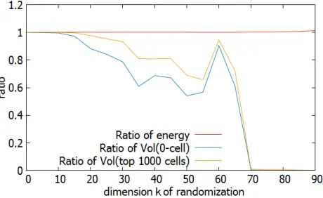
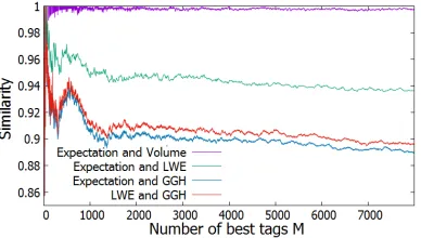
In practice, it is more efficient to rely on the expectation, because it is faster to evaluate. Fig. 4 shows how similar are the best tags with respect to one indi-cator compared to another: to compare two setsAandB formed by the bestM
tags, the graph displays #(A∩B)/M. For instance, the top curve confirms the
ex-Fig. 4. Similarity between optimal sets of tags, depending on the objective function.
perimental result of [10] that themtagstwhich maximize vol(CN(t)∩Balln(R)) are almost the same as the ones which minimize the expectationE{CN(t)}. The
top second curve shows that the best tags that maximize the LWE probabil-ity are very close to those minimizing the expectation. The bottom two curves compare with the finite noise distribution arising in GGH challenges [23] (see Sect. B for details). In all cases, at most 10% of the best tags are different, and more importantly, we report that the global success probabilities are always very close, with a relative error typically≤1%.
We conclude that in practice, the expectation is a very good indicator to select the best tags for the distributions studied in Sect. 5.6.
6.2 Limits of Orthogonal Enumeration
Pn i=1 t2 i 4 + ti 4 + 1 12
kb?ik2,by noticing that
E{CN(t)}was the squared distance
between a target point and a special lattice with a known orthogonal basis. This allowed to find allt∈Nnsuch that
E{CN(t)} ≤Rfor anyR, using a variant [10,
Alg. 6] of enumeration. And by using a binary search based on an early-abort variant, it was also possible to find anRyielding slightly more thanmsolutions. [10, Sect. 6] reported that this algorithm worked very well in practice: if `
is the number of t ∈ Nn such that E{CN(t)} ≤ R, the number of nodes L of
the enumeration algorithm [10, Alg. 6] seemed to be bounded byO(`n), perhaps even `×n. This was in contrast with the usual situation where the number of nodes of the enumeration tree is exponentially larger than the number of solutions. However, no rigorous result could be proved in [10], leaving it as an open problem to show the efficiency of [10, Alg. 6].
Surprisingly, we solve this open problem of [10] in the negative. More pre-cisely, we show that there are cases where the number of nodes L of enumer-ation [10, Alg. 6] is exponentially larger than the number of solutions `. To see this, consider the orthogonal lattice Zn with the canonical basis. Then:
E{CN(t)}=
Pn i=1 t2 i 4 + ti 4 + 1 12
. But we have:
Lemma 8. Let R = n
12 + 1 2 and n
0 =bn/10c. Then the number ` of t ∈
Nn
such that Pni=1t2i
4 + ti 4 + 1 12
≤ R is exactly n + 1. But the number `0 of (xn−n0+1, . . . , xn)∈Nn
0
such thatPni=n−n0+1 x2 i 4 + xi 4 + 1 12
≤R is≥2n0.
Proof. For the choiceR=12n +12, we havePni=1t2i
4 + ti 4 + 1 12
≤Rif and only if all theti’s are equal to zero, except at most one, which must be equal to one.
Furthermore, for any (xn−n0+1, . . . , xn)∈ {0,1}n 0
, we have: n
X
i=n−n0+1 x2 i 4 + xi 4 + 1 12 ≤n0
1 2 + 1 12 ≤ n 10 7 12 = 7n
120 < R.
u t
It follows in this case that the number of nodesLof the enumeration algorithm [10, Alg. 6] for thatRis at least exponential inn, though the number of solutions is linear inn.
6.3 Solving Linear Optimization
We show that a slight modification of orthogonal enumeration can solve the more general problem of linear optimization essentially optimally. This is based on two key ideas. The first idea is that when solving linear optimization, we may assume without loss of generality that each function f(i,) is sorted by increasing value, with a starting value equal to zero, which changes the tree:
that for both the expectation E{CN(t)} = Pn i=1 t2 i 4 + ti 4 + 1 12
kb?ik2 and for −Pni=1logerf√1
2σ· ti+1
2 · kb ? ik
−erf√1 2σ ·
ti
2 · kb ? ik
, the values of f(i,) are already sorted. For instance, t2i
4 + ti
4 + 1
12 is an increasing function ofti. The second idea is that we may assume to simplify thatf has integral values, which allows us to bound the running time of dichotomy. This is not directly true for the expectationE{CN(t)}=
Pn i=1 t2 i 4 + ti 4 + 1 12
kb?ik2. However, because we deal with integer lattices, the basisBis integral, thekb?
ik2’s are rational numbers with denominator covol(L(b1, . . . ,bi−1))2, so we can transform the expectation into an integer, by multiplying with a suitable polynomial-size integer.
First, we present a slight modification Alg. 3 of [10, Alg. 6], whose running time is provably essentially proportional to the number of solutions:
Theorem 11. Assume that f : {1, . . . , n} ×N → R satisfies f(i,0) = 0 and
f(i, j)≥ f(i, j0) for all i and j > j0. Given as input a number R > 0, Alg. 3 outputs all (v1, . . . , vn) ∈ Nn such that Pni=1f(i, vi) ≤ R using O(nN + 1) arithmetic operations and ≤(2n−1)N+ 1 calls to the functionf(), where the numberN is the number of (v1, . . . , vn)∈Nn such thatPni=1f(i, vi)≤R. Proof. To analyze the complexity of Alg. 3, letnk denote the number of times we enter Lines 3–18, depending on the value of k, which is ≥ 1 and ≤ n at each Line 3. Then nk can be decomposed as nk =ak+bk, where ak (resp.bk) denotes the number of times we enter Lines 5–10 (resp. Lines 12–17). Notice that an+1 = 0 and a1 is exactly the number N of (v1, . . . , vn)∈Nn such that
Pn
i=1f(i, vi) ≤R. And if 1< i ≤n, then ai is the number of times that the variablekis decremented fromitoi−1. Similarly,bn= 1, and if 1≤i≤n, then
bi is the number of times that the variablekis incremented fromitoi+ 1. By Line 1 (resp. 14), the initial (resp. final) value ofkisn(resp.n+ 1). Therefore, for any 1≤i≤n−1, the number of timeskis incremented fromitoi+ 1 must be equal to the number of timeskis decremented fromi+ 1 toi, in other words:
bi=ai+1. Thus, the total number of loop iterations is: n
X
i=1
ni = n X
i=1
(ai+bi) =N+ 1 + 2 n X
i=2
ai.
Note that becausef(i,0) = 0, any partial assignmentPni=i
0f(i, vi)≤Rcan be
extended to a larger partial assignment Pni=1f(i, vi) ≤R, which implies that
a1≥a2≥. . . an. It follows that the total number of loop iterations is: n+1
X
i=1
ni≤N+ 1 + 2(n−1)N = (2n−1)N+ 1.
For each loop iteration (Lines 3–18), the number of arithmetic operations per-formed isO(1) and the number of calls tof() is exactly one. It follows that the total number of arithmetic operations isO(nN+ 1) and the number of calls to
We showed that the number of nodes in the search tree is linear in the number of solutions. Next, we present Alg. 4, which is a counting version of Alg. 3:
Theorem 12. Assume that f : {1, . . . , n} ×N → R satisfies f(i,0) = 0 and
f(i, j)≥ f(i, j0) for all i and j > j0. Given as input two numbers R >0 and
M > 0, Alg. 4 decides if is N ≥ M or N < M, where N is the number of (v1, . . . , vn) ∈ Nn such that Pni=1f(i, vi) ≤ R. Furthermore, if N ≥ M, the number of arithmetic operations is O(N), and otherwise, the number of arith-metic operations is O(nN+ 1), and the algorithms outputs N.
Proof. Similarly to the proof of Th. 11, let nk denote the number of times we enter Lines 3–17, depending on the value of k, which is ≥ 1 and≤ n at each Line 3. Thennk can be decomposed asnk =ak+bk, whereak(resp.bk) denotes the number of times we enter Lines 5–9 (resp. Lines 11–16).
LetM be the number of (v1, . . . , vn)∈ Nn such that Pni=1f(i, vi)≤R. If
M ≤N, then Alg. 4 will perform the same operations as Alg. 3 (except Line. 6), so the cost isO(nM+1)≤O(nN+1) arithmetic operations. Otherwise,M > N, which means that the while loop will stop after exactly N iterations, and the
total number of operations is thereforeO(N). ut
Our main result states that if the function f is integral, given any M, Alg. 5 finds the bestN assignments in time M whereM ≤N ≤(n+ 1)M:
Theorem 13. Assume that f : {1, . . . , n} ×N → N satisfies f(i,0) = 0 and
f(i, j)< f(i, j0) for alli and j > j0. Assume that f(i, j)≤jO(1)2nO(1). Given as input a number M >1, Alg. 5 outputs theN assignments (v1, . . . , vn)∈Nn
which minimizePni=1f(i, vi)in timeO(n(n+ 1)M) +nO(1)+O(log2M), where the numberN satisfies: M ≤N ≤(n+ 1)M.
Proof. We have the following invariant at the beginning of each loop itera-tion: the number of (v1, . . . , vn) ∈ Nn such that Pni=1f(i, vi) ≤ R0 is < M, and the the number of (v1, . . . , vn) ∈ Nn such that Pni=1f(i, vi) ≤ R1 is ≥ M. Initially, this holds because the number of (v1, . . . , vn) ∈ Nn such
that Pni=1f(i, vi) ≤ 0 is 1 and the number of (v1, . . . , vn) ∈ Nn such that
Pn
i=1f(i, vi) ≤ Pn
i=1f(i,dM
1/ne) is ≥ (M1/n)n =M. Furthermore, the loop preserves the invariant by definition of the loop. Since the length R1 −R0 decreases by a factor two, it follows that the number of loop iterations is ≤log2(
Pn
i=1f(i,dM 1/ne)).
Furthermore, Alg. 5 uses negligible space, except that the output is linear in
M: the best tags are actually output as a stream. If we sort theN tags, which requires space, we could output exactly the best M tags.
Algorithm 3Enumeration of low-cost assignments
Input: A functionf :{1, . . . , n} ×N→R≥0such thatf(i,0) = 0 andf(i, j)≥
f(i, j0) for all iandj > j0; a boundR >0.
Output: All (v1, . . . , vn)∈Nn such thatPni=1f(i, vi)≤R. 1: v1=v2=· · ·=vn= 0 andρn+1= 0 andk=n
2: whiletruedo
3: ρk =ρk+1+f(k, vk) // cost of the tag(0, . . . ,0, vk, . . . , vn) 4: if ρk≤R then
5: if k= 1 then
6: return(v1, . . . , vn); (solution found) 7: vk←vk+ 1
8: else
9: k←k−1 andvk ←0// going down the tree
10: end if
11: else
12: k←k+ 1// going up the tree 13: if k=n+ 1then
14: exit (no more solutions) 15: else
16: vk←vk+ 1
17: end if
18: end if
19: end while
7
Quantum Speed-up of Discrete Pruning
We present a quadratic quantum speed-up for discrete pruning, namely:
Theorem 14. There is a quantum algorithm which, givenε >0, a numberM >
0, and an LLL-reduced basisB of a full-rank latticeLinZn, outputs the shortest non-zero vector inL∩P in timeO(n2√M)poly(log(n),log(M),log(1/), β)with error probabilityε. Here,βdenotes the bitsize of the vectors ofB,P =∪t∈UCN(t)
whereCN()is the natural partition with respect toB,U is formed by the N tags t minimizing E{CN(t)}, for some M ≤ N ≤ 32n2M with probability at least
1−ε/2. If the algorithm is further given a target u ∈ Zn, it also outputs the
shortest vector in (L−u)∩P.
Algorithm 4Counting low-cost assignments
Input: A functionf :{1, . . . , n} ×N→R≥0such thatf(i,0) = 0 andf(i, j)≥
f(i, j0) for all iandj > j0; a boundR >0 and a numberM ≥0.
Output: Decide if the number of (v1, . . . , vn)∈Nn such thatPni=1f(i, vi)≤R is≥M or < M.
1: v1=v2=· · ·=vn= 0 andρn+1= 0 andk=nandm= 0 2: whilem < M do
3: ρk =ρk+1+f(k, vk) // cost of the tag(0, . . . ,0, vk, . . . , vn) 4: if ρk≤R then
5: if k= 1 then
6: m←m+ 1 and vk←vk+ 1 (one more solution) 7: else
8: k←k−1 andvk ←0// going down the tree
9: end if
10: else
11: k←k+ 1// going up the tree 12: if k=n+ 1then
13: returnm < M // no more solutions 14: else
15: vk←vk+ 1
16: end if
17: end if
18: end while
19: returnm≥M
Algorithm 5Enumeration of lowest-cost assignments
Input: A functionf :{1, . . . , n} ×N→R≥0such thatf(i,0) = 0 andf(i, j)≥
f(i, j0) for all iandj > j0; a numberM >0.
Output: Output the N assignments (v1, . . . , vn) ∈ Nn that minimize
Pn
i=1f(i, vi), whereM ≤N ≤nM. 1: R0←0 andR1←
Pn
i=1f(i,dM 1/ne); 2: whileR0< R1−1 do
3: Call Alg. 4 with R=b(R0+R1)/2eandM 4: if number of solutions≥M then
5: R1←R 6: else
7: R0←R 8: end if
9: end while
10: Call Alg. 3 withR1.
tree interpretation. Alg. 3 can be seen as a backtracking algorithm on a tree T(R), where each node can be encoded as (∗,· · ·,∗, vk,· · ·, vn). The root is encoded as (∗,· · ·,∗). Given a node (∗,· · ·,∗, vk,· · · , vn), if k = 1, then it is a leaf. If Pni=kf(i, vi) > R, then it is also a leaf. If Pni=kf(i, vi) ≤ R, then its children are (∗,· · ·,∗, vk−1, vk,· · ·, vn), wherevk−1 can take all integer val-ues between 0 and ρvk,···,vn. Here ρvk,···,vn is the smallest integer such that
f(i−1, ρvk,···,vn) +
Pn
i=kf(i, vi)> R. In case of discrete pruning,f is quadratic. We can computeρvk,···,vn and build the black-box onT(R).
7.1 Determining the best cells implicitly
Given a number M > 0, Alg. 5 finds (in time essentially M) the best
N vectors t ∈ Nn (for some N close to M) minimizing E{CN(t)} =
Pn i=1
t2
i
4 + ti
4 + 1 12
kb?
ik2 by minimizing instead the function:
g(v1,· · ·, vn) = n X
i=1
f(i, vi) = n X
i=1
vi(vi+ 1)kb?ik 2=
n X
i=1
αivi(vi+ 1).
This is done by finding a suitable radius R by dichotomy, based on logarith-mically many calls to Alg. 4 until the number of solutions is close to M, and eventually enumerating the marked leaves of a search tree by Alg. 3. Both Alg. 3 and Alg. 4 can be viewed as algorithms exploring a tree T(R) depending on a radiusR >0: Alg. 4 decides if the number #S(T(R)) of marked leaves (i.e.the number of outputs returned by Alg. 3) is ≥or <than an input number; Alg. 3 returns all the marked leaves.
This tree interpretation gives rise to Alg. 6, which is our quantum analogue of Alg. 5 with the following differences: we are only interested in finding a suit-able radius R such thatN = #S(T(R)) is close to M up to a factor of 32n2, with correctness probability at least 1−ε/2, because enumerating all the marked leaves would prevent any quadratic speed up. We replace Alg. 4 by the quantum tree size estimation algorithm of [9]: this gives a quadratic speed up, but approx-imation errors slightly worsen the upper bound on N. The input (α1,· · · , αn) of Alg. 6 corresponds to (kb?1k2,· · ·,kb?nk2), where (b1,· · ·,bn) is an integer basis. We know that (kb?1k2,· · · ,kb?nk2) ∈ Qn, but by suitable multiplication preserving polynomial sizes, we may assume that (kb?
1k2,· · · ,kb?nk2)∈Nn. The order between the kb?
ik2’s doesn’t matter in our analysis. We can assume that kb?
1k2≤ · · · ≤ kb?nk2. We show that Alg. 6 finds a radiusRcorresponding to the bestM cells in approximately √M quantum operations:
Theorem 15. The output R of Alg. 6 satisfies M ≤ #S(T(R)) ≤ 32n2M with probability ≥ 1 − ε/2. Alg. 6 runs in quantum time
Algorithm 6Computing implicitly the best cells quantumly
Input: ε, M >0 and (α1,· · · , αn)∈Nnwithα1≤ · · · ≤αnsuch that the input
f :{1,· · ·, n} ×N→Nof Alg. 3 satisfies f(i, x) =αix(x+ 1)
Output: R such thatM ≤#S(T(R))≤32n2M with probability≥1−ε 1: r ← dlog2(
Pn
i=1f(i,d(4nM)
1/ne))e and R ← Pn
i=1f(i,d(4nM)
1/ne) and
R0←0 andR1←R 2: whileR1−R0>1 do
3: CallTreeSizeEstimation(T2(R),16n2M,1/2, εr/2,2)
4: if the answer is ”T2(R) contains more than 16n2M vertices”then 5: R1←RandR← b(R0+R1)/2e
6: else if the answer is ”T2(R) contains ˆT vertices” with ˆT < 3(2n−1)M
then
7: R0←RandR← b(R0+R1)/2e 8: else
9: ReturnR
10: end if
11: end while
12: ReturnR0
7.2 Finding the best lattice vector
We now know R such that the number N of (v1,· · ·, vn) ∈ Nn which
satis-fies Pni=1f(i, vi) ≤R is in [M,32n2M] with probability at least 1−ε/2. All these solutions are leaves of the tree T(R) and they form the set U of the bestN tags minimizingtminimizing E{CN(t)}. LetP =∪t∈UCN(t) whereCN()
is the natural partition with respect to the input basis B. We would like to find a shortest non-zero vector in L∩P for the SVP setting, or the shortest vector in (L−u)∩P in the CVP setting, when we are further given tar-get u ∈ Zn. To do this, we notice that it suffices to apply FindMin2 (in
App), provided that the basis (b1,· · · ,bn) is LLL-reduced. More precisely, we call FindMin2(T(R),P, h,kb1k2, d,32n2M, ε/2). Here P is the predicate which returns true on a node iff it is a leaf encoded as (x1,· · · , xn) such that
g(x1,· · ·, xn) = Pn
i=1f(i, xi)≤R.hV(x1,· · ·, xn) is the predicate which indi-cates if the square of the norm of the lattice vector in the cell of tag (x1,· · · , xn) is≤V. The time complexity isO(n2√Mpoly(log(n),log(M),log(1/ε), β)).
Since the subroutine of determining the best cells and the one of finding a shortest non-zero vector, both have an error probability ε/2, by union bound, the total error probability isε. We thus have proved Th. 14.
7.3 The Case of Extreme Pruning
Given m LLL-reduced bases (B1,· · ·,Bm) of the same integer lattice L of rank n, we define for each basis Bi a function gi : Nn → Q such that
gi(x1,· · ·, xn) = Pn
j=1kb ?
i,jk2xi(xi + 1), where (b?i,1,· · ·,b?i,n) is the Gram-Schmidt orthogonalization of the basis Bi. Here, we want to first find the
poly(n) ∗ M best cells with respect to all of the functions gi altogether, and then find the shortest vector in these cells. Both steps have complex-ity O(√Mpoly(n,logM,log 1/ε, β)), where ε is the total error probability and whereβ is the bitsize of the vectors of the input bases.
Theorem 16. There is a quantum algorithm which, givenε >0, a numberM >
0, andmLLL-reduced bases(B1,· · ·,Bm)of ann-rank integer latticeL, outputs the shortest non-zero vector in L∩P in time O(√Mpoly(n,logM,log 1/ε, β)) with error probability ε. Here, β denotes the maximum bitsize of the vectors of all given bases, P =∪(i,t)∈UCN(i,t) where CN(i,·) is the natural partition with
respect to Bi, U is formed by the N tuples (i,t)∈ {1,· · ·, m} ×Nn minimizing
gi(t) among all tuples, for some N = poly(n)∗ M with probability at least 1−ε/2. If the algorithm is further given a target u ∈ Zn, it also outputs the
shortest vector in (L−u)∩P.
The main idea of the proof is the following. For each basis Bi, there is a back-tracking tree with respect to the function gi as we explained in the previous section. We put all these trees together and obtain one single tree. We first ap-ply the TreeSizeEstimation algorithm several times to find a good common radiusR for all functions gi by dichotomy, such that the total number of good cells in all trees is poly(n)∗M. After that, we apply FindMin2 to find the shortest vector among all these cells. Remark that in the previous section, we required the functiong to have integral values, and this was achieved by multi-plying all kb?ik2 by a common denominator. Instead, we here want to keep the output rational, which is proved sufficient by the following lemma:
Lemma 9. Given a basis(b1,· · · ,bn)of an integer latticeL,g:Nn→Qsuch
thatg(x1,· · · , xn) = Pn
i=1kb ?
ik2xi(xi+1), we denoteT(R)the backtracking tree for finding all solutions of g(x1,· · · , xn) ≤R, T2(R) the corresponding binary tree. For all R ∈R+,#S(T
2(R+δ))≤2n#S(T2(R)), where δ= Qn1
i=1∆i and
∆i= covol(b1,· · ·,bi)2= Qi
j=1kb ? ik
2.
The proof of this lemma is the same as the proof of Lemma 10 in the App. by noticing thatQni=1∆i is a common denominator of allkb?ik2.
For each basis Bi, we define δi as in Lemma 9. In the dichotomy step, we stop when the difference of the two terms is smaller than minj∈{1,···,m}δj. The other steps are the same as in the previous section.
Acknowledgements

![Fig. 6. (Left) The graph of Pre[∥e∥2 = r2] for GGH-200’s noise; (Right) Theoreticaland experimental success probability on PBKZ-60 bases of the GGH-200 lattice.](https://thumb-us.123doks.com/thumbv2/123dok_us/7980186.1323574/34.612.137.567.307.452/graph-right-theoreticaland-experimental-success-probability-bases-lattice.webp)