Modeling intergranular cracking in polycrystalline aggregates:
explicit account for grain boundaries with cohesive zone approach
Igor Simonovski1, Leon Cizelj2, Gangadhar Machina3and Mihaela Irina Uplaznik4
1 European Commission, DG JRC, Institute for Energy and Transport, P.O. Box 2, NL-1755
ZG Petten, The Netherlands ([email protected])
2Professor, Joˇzef Stefan Institute, Jamova cesta 39, SI-1000 Ljubljana, Slovenia ([email protected])
3European Commission, DG JRC, Institute for Energy and Transport, P.O. Box 2, NL-1755 ZG
Petten, The Netherlands ([email protected])
4Joˇzef Stefan Institute, Jamova cesta 39, SI-1000 Ljubljana, Slovenia ([email protected])
ABSTRACT
Understanding and controlling early damage initiation and evolution are amongst the most important issues in nuclear power plants. Intergranular cracking has been known to occur in both austenitic steels and nickel based alloys. In this work a grain-level scale model is pre-sented for modeling interganular cracking. Grains and grain boundaries are modeled explicitly. Grain boundary damage initiation and evolution is included by employing the cohesive zone approach. Both cohesive elements and cohesive surfaces are explored and compared. Cohe-sive surface approach is simpler to implement while the coheCohe-sive elements make the tracking of the damage initiation and evolution easier. The behaviour under simple isotropic elastic and more complex crystal plasticity constitutive laws for grains is studied. For the studied cases the cohesive surface approach with linear tetrahedron elements proved to be numerically much more stable compared to cohesive elements and cohesive surfaces with quadratic tetrahedron el-ements. For the cohesive elements and the cohesive surfaces with linear tetrahedron elements, the increase in the cohesive stiffness has basically no effect. For the cohesive surfaces with quadratic tetrahedron elements, the effect is positive at small mesh density.
INTRODUCTION
The first part of the paper presents the used finite element model with boundary conditions and material parameters. The next section deals with the numerical example and results. Rec-ommendations and conclusions are given at the end.
THE FINITE ELEMENT MODEL
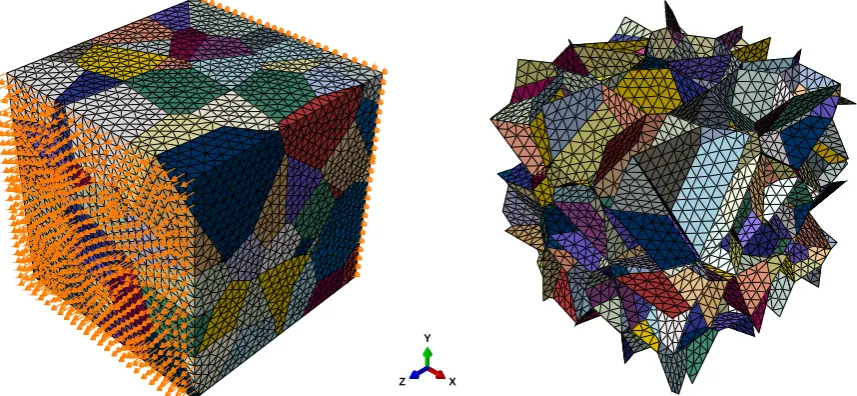
A polycrystalline aggregate is modeled using 3D Voronoi tessellation with Wigner-Seitz cells [6], see Fig. 1. It contains 150 grains and 805 grain boundaries. Two mesh densities are used with average element size of 0.05 mm or 0.025 mm. The size of the model is 1x1x1 mm. A conformal mesh is created between the grains and grain boundaries. Details of the meshing procedure have been previously reported [7]. Linear 4-node or modified 10-node tetrahedron elements (ABAQUS types C3D4, C3D10M) are used for meshing grains while grain bound-aries are either modeled using cohesive elements (linear triangular prism elements, ABAQUS type COH3D6) or cohesive surfaces. The crystallographic orientations of grains are randomly distributed [8]. In this work a simplification of grain boundary modelling is applied with all the grain boundaries having the same material properties.
X Y
Z
Figure 1: Coarse FEM model with average element size of 0.05 mm. Different colors indicate different grains (left) and grain boundaries (right).
Loads and boundary conditions
Tensile displacement load of 0.035 mm is applied to the front surface (max(Z) coordinates, Fig. 1). This results in a significant specific deformation in Z direction (z = 0.035) and ensures
grain boundary crack initiation and propagation. Displacement load is used instead of the stress load to limit the energy flow into the model. With tensile stress load two neighbouring grains with a degraded grain boundary would continue to move apart even after the boundary has fully degraded. A loading step time oftstep=1.0 s is used to apply the full tensile load displacements.
Material parameters: grains
The material is assumed to be similar to AISI 304 stainless steel. Two types of constitutive laws are used: isotropic elasticity and crystal plasticity. For isotropic elasticity (IE) Young modulus and Poisson ratio are taken as 204600 MPa and 0.3. More complex models of grain boundary crack initialization and propagation use crystal plasticity (CP) constitutive law as described below.
For CP constitutive law the anisotropic elasticity and crystal plasticity are used as descried in [9]. Elastic constants of a single crystal AISI 304 stainless steel are [10]: Ciii=204 600 MPa, Ciijj=137 700 MPa and Cijij=126 200 MPa. The crystal plasticity parameters were initially
taken from the literature [11] where they were obtained by fitting the computed macroscopic response of a polycrystal aggregate to a measured tensile test of a polycrystal sample. However, Pierce et al. hardening law in [11] was replaced by Bassani et al. hardening law [9] for better stability: h0= 75 MPa, τs= 75 MPa, τ0= 150 MPa, hs=30 MPa. Crystal plasticity was
imple-mented as a user-subroutine [9] into the finite element code ABAQUS and includes versions for small deformation theory and rigorous theory of finite-strain and finite-rotation. The latter is used in this work.
Material parameters: grain boundaries
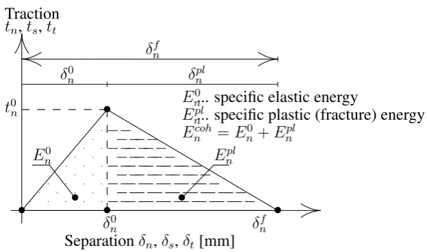
The cohesive zone approach [1, 2] with damage initiation and evolution as implemented in ABAQUS is used as a constitutive law for the grain boundaries. The traction-separation response is given by Fig. 2. The indicesn,sandtdenote the normal and two orthogonal shear directions. The normal direction always points out of the plane of the cohesive element/surface. The tractions of a cohesive element/surface,tn,tsandttare given by Eq. (1).Knn,KssandKtt
are the stiffnesses in the normal and two shear directions.
tn ts tt
=
Knn 0 0
0 Kss 0
0 0 Ktt
n s t
(1)
Damage evolutionD(δ)is defined by Eq. (2) for the normal direction (and both shear direc-tions).
D(δ) =
0 ; δ < δ0
n δnf(δ−δn0)
δ(δnf−δn0)
; δ ≥δn0
(2)
The actual load-carrying capability of the cohesive element in the normal direction would then betn= [1−D(δ)]Knn·nand correspondingly for the two shear directions.
Grain boundary stiffnesses are taken as: Knn=204 600 MPa andKss = Ktt = E/[2(1 + ν)]=78 692.3 MPa. n, s and t are defined as δn/T0, δs/T0, δt/T0, where T0 stands for the
constitutive thickness of a cohesive element. This is mostly different from the geometric thick-ness which is typically close or equal to zero. In this work a value of T0 = 1.0·10−3mm
is used. Also, let us assume that the specific deformation at damage initialization point is
. . . . . . . . . . . . . . . . . . . . . . . . . −−−−−−−−−−−−−−−−−−−−−−−−−−−−−− −−−−−−−−−−−−−−−−−−−−−− −−−−−−−−−−−−−−−− −−−−−−−−−− −− ... ... ... ... ... ... ... ... ... ... ...... ...... ...... ...... ...... ...... ...... ... . . . . . . . . . . . . . . . . . . . . . . . . . . . . . . . . . . . . . . . . . . . . . . . . . . . . . . . . . . . . . . . . . . . . . . . . . . . . . . . . . . . . . . . . . . . . . . . . . . . . . . . . . . . . . . . . . . . . . . . . . . . . . . . . . . . . . . . . . . . . . . . . . . . . . . . . . . . . . . . . . . . . . . . . . . . . . . . . . . . . . . . . . . . . . . . . . . . . . . . . . . . . . . . . . . . . . . . . . . . . . . . . . . . . . . . . . . . . . . . . . . . . . . . . . . . . . . . . . . . . . . . . . . . . . . . . . . . . . . . . . . . . . . . . . . . . . . . . . . . . . . . . . . . . . . . . . . . . . . . . . . . . . . . . . . . . . . . . . . . . . . . . . . . . . . . . . . . . . . . . . . . . . . . . . . . . . . . . . . . . . . . . . . . . . . . . . . . . . . . . . . . . . . . . . . . . . . . . . . . . . . . . . . . . . . . . . . . . . . . . . . . . . . . . . . . . . . . . . . . . . . . . . . . . . . . . . . . . . . . . . . . . . . . . . . . . . . . . . . . . . . . . . . . . . . . . . . . . . . . . . . . . . . .. . . . . . . . . . . . . . . . . . . . . . . . . . . . . . . . ... ... ... ... • • • • • • ... ... ... ... ... ... ... ... ... ... ... ... ... ... ... ... ... ... ... ... ... ... ... ... ... ... ... ... ... ... ... ... ... ... ... ... ... ... ... ... ... ... ... ... ... ... ... ... ... ... ... ... ... ... ... ... ... ...... ... ... ... ... . . . . . ... . . . . . . . . . . . . . . . . . . . . . . . . . . . . . . . . . ... . . . . . . . . . . . . . . . . . . . . . . . . . . . . . . . . . . . . . . . . . . . . . . . . . . . . . . . . . . . . . . . . . . . . . . . . . . . . . . . . . . . . . . . . . . . . . . . . . . . . . . . . . . . . . . . . . . . . . . . . . . . . . . . . . . . . . . . . . . . . . . . . . . . . . . . . . . . . . . . . . . . . . . . . . . . . . . . . . . . . . . . . . . . ... ... t0 n Traction
tn,ts,tt
δpl n δ0
n
δnf
En0 Enpl
δ0
n δnf
Separationδn,δs,δt[mm] E0
n Enpl Ecoh
n =En0+Enpl
... specific elastic energy
... specific plastic (fracture) energy
Figure 2: Example of traction-separation response.
is t0
n = Knn · 0n=204.6 MPa, almost equal to 0.2 % offset yield stress of AISI 304 which is
205 MPa [12].
Other grain boundary material parameters are determined following the grain boundary frac-ture energy approach in [5]. The grain boundary fracfrac-ture energy, Epl, can be related to the
surface energy,γS and grain boundary energy,γGB through Eq. (3). The factor 2 is because 2
surfaces are created during fracture.
Epl = 2γS−γGB (3)
Experimentally reported values for surface energies of Fe, Ni and Cr are [13]: γSF e = 2.5·
10−3mJ/mm2, γ
SN i = 2.5·10
−3mJ/mm2 andγ
SCr = 2.4·10
−3mJ/mm2, respectively. For a
typical AISI 304 stainless steel with 18 % of Cr, 8 %Ni, 2 % Mn, combined 1 % of C, Mn, P, S, Si, Na and balance of Fe a value ofγSAISI304 = 2.5·10
−3mJ/mm2 seems a reasonable choice.
Since the ratioγGB/γs is typically 1.2 to 1.5, we can estimate theγGB to be between3·10−3
and3.75·10−3mJ/mm2. Resistant grain boundaries would have lowerγ
GB to have larger grain
boundary fracture energy compared to susceptible grain boundaries, Eq. (3). Let us assume that
γGBres =γGBsusc/10. This is relative conservative ratio considering that the reported ratios can
be up to 41 [14]. Hence, we can estimate:
Esuscpl = 2·2.5−(3up to3.75)·10−3 = (1.25up to2.0)·10−3mJ/mm2 (4)
For simplification, we are going to treat all the grain boundaries as susceptible. Let us take the upper valuesEpl
susc= 2.0·10
−3mJ/mm2. Since the elastic energy of the traction-separation
response is En0 = 12t0nδ0n = 1.023·10−4mJ/mm2, we can now determine the cohesive energy (area under the traction separation response):
Esusccoh =En0 +Esuscpl = 1.023·10−4+ 2.0·10−3 = 2.1023·10−3mJ/mm2, (5)
SinceEcoh = 12tn0δnf we can also computeδnf. In the formulations above, we have assumed that a cohesive element is only deformed in the normal direction.
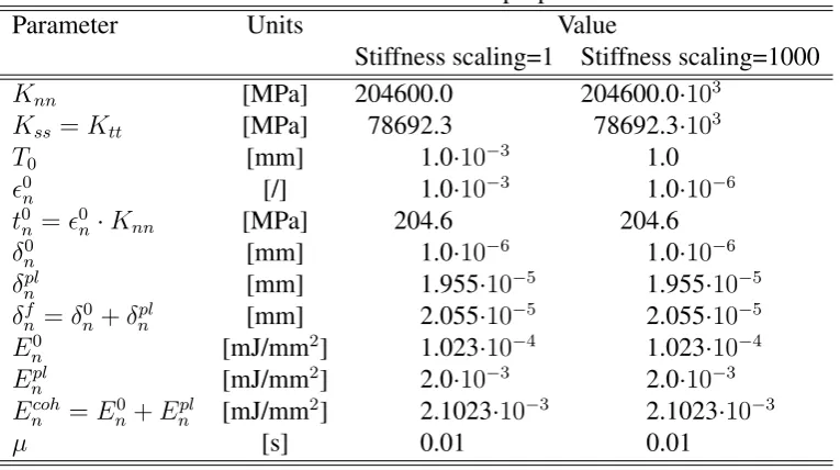
fracture energies and the maximal stresst0nare equal to the ones for the basic case. In order to do so, we need to increase the constitutive thickness by a factor of 1000. Table 1 summarizes the cohesive element properties used for the basic and increased stiffness cases.
Table 1: Cohesive element properties.
Parameter Units Value
Stiffness scaling=1 Stiffness scaling=1000
Knn [MPa] 204600.0 204600.0·103
Kss =Ktt [MPa] 78692.3 78692.3·103
T0 [mm] 1.0·10−3 1.0
0
n [/] 1.0·10
−3 1.0·10−6
t0n=0n·Knn [MPa] 204.6 204.6
δ0
n [mm] 1.0·10
−6 1.0·10−6
δpl
n [mm] 1.955·10
−5 1.955·10−5
δnf =δn0 +δnpl [mm] 2.055·10−5 2.055·10−5
En0 [mJ/mm2] 1.023·10−4 1.023·10−4
Epl
n [mJ/mm2] 2.0·10
−3 2.0·10−3
Encoh =En0+Enpl [mJ/mm2] 2.1023·10−3 2.1023·10−3
µ [s] 0.01 0.01
CRACK EVOLUTION
The effect of two types of cohesive approaches is investigated on the stability of the numer-ical simulations: cohesive elements and cohesive surfaces. Isotropic elasticity (IE) and crystal plasticity (CP) constitutive laws for grains are used and stiffness scaling of 1 and 1000.
Viscous regularization
To improve the convergence, viscous stiffness degradation,Dν, is used instead ofD. The
two are related through Eq. (6) where µis the viscosity parameter representing the relaxation time of the viscous system andDis the degradation variable evaluated in the inviscid backbone model, Eq. (2) [15].
˙
Dν =
1
µ(D−Dν) (6)
For a linearly time dependent separation (δn(t) = δ
f n
tstep·t) an analytical expression forDν can
be derived [16], Eq. (7). Fig. 3 demonstrates the corresponding effect of viscous regularization on the traction-separation response.
Dν(t) =
ifδ(t)≤δ0
n then: 0
ifδ(t)> δ0
n then: δfn
δnf−δn0
−e−tµ 1
µ tstepδ0n
δnf−δn0
ln|t|+ P∞ i=1
t µ
i 1 i·i!
+Ce−tµ
C = 1
µ
tstepδ0n
δnf −δn0
ln
tstepδn0
δnf
+
∞ X
i=1
tstepδ0n
µδnf !i
1
i·i!
−e
tstepδ0n
µδnf δ
f n δfn−δn0
(8)
0.0 0.1 0.2 0.3 0.4 0.5 0.6 0.7 0.8 0.9 1.0 1.1
Relative displacementδn/δnf [/]
0.00 0.25 0.50 0.75 1.00 1.25 1.50 1.75 2.00 2.25 2.50 2.75 3.00
Relati
v
e
traction
tn
/t
0 n
[/]
µ=0.0
µ=1 % oftstep µ=5 % oftstep
µ=10 % oftstep
µ=20 % oftstep
... ... ... ...
... ... ...
...
......
......
......
...... ... ...
... ...
... ...
... ... ...
... ...
... ...... ...
... ...... ...
... ...... ...
... ...... ...
... ...... ... ... ... ... ... ...
... ...
... ...
... ...
... ... ...
... ...
... ...
... ......
... ... ... ...
... ...... ...
... ...... ...
... ...... ... ... ... ...
... ...
... ...
... ...
... ...
... ... ... ...
... ...
... ...
... ...
... ...
...... ......
... ... ... ...
... ...
... ...... ... ... ... ...
... ...
... ...
... ...
... ...
... ...
... ...
...
... ... ... ...... ...
... ...
... ...
... ...
... ...
... ...
... ...
... ...
...... ...
...... ......
Figure 3: The effect of viscous regularization [16]. δ0n/δfn=0.048.
In this work a viscosity parameter equal to 1 % of the step time is used:µ= 0.01·tstep=1.0 s,
see Table 1. This ensures only a small impact on the traction-separation response, see Fig. 3.
Table 2: Achievable times [s] for the investigated cases. Isotropic elasticity (IE)
El.size=0.05 mm El.size=0.025 mm
Stiff.scaling 1 Stiff.scaling 1000 Stiff.scaling 1 Stiff.scaling 1000
Coh. elements 0.0257 0.0248 0.0260 0.0247
Coh. surfaces C3D4 1.0000 1.0000 1.0000 1.0000
Coh. surfaces C3D10M 0.2360 1.0000 0.2280 0.1020
Crystal plasticity (CP)
El.size=0.05 mm El.size=0.025 mm
Stiff.scaling 1 Stiff.scaling 1000 Stiff.scaling 1 Stiff.scaling 1000
Coh. elements 0.0208 0.0208 0.0250 0.0250
Coh. surfaces C3D4 1.0000 1.0000 1.0000 1.0000
Coh. surfaces C3D10M 0.9670 1.0000 1.0000 0.0926
Results
IE, C3D4
(Avg: 75%) S, Mises
0.00 25.00 50.00 75.00 100.00 125.00 150.00 175.00 200.00 225.00 250.00 275.00 300.00
CP, C3D4
IE, C3D4
(Avg: 75%) S, Mises
0.00 25.00 50.00 75.00 100.00 125.00 150.00 175.00 200.00 225.00 250.00 275.00 300.00
CP, C3D4
IE, C3D10M
(Avg: 75%) S, Mises
0.00 25.00 50.00 75.00 100.00 125.00 150.00 175.00 200.00 225.00 250.00 275.00 300.00
CP, C3D10M
IE cases stop when the tensile displacement load results in σz ≈180 MPa (stiff.scaling 1)
or σz ≈173 MPa (stiff.scaling 1000), which is quite close to the maximum tensile stress in a
cohesive element (t0
n=204.6 MPa). For IE cases the overall amount of damage in the cohesive
elements at the end of simulation was very low. Values of damage above 0.1 (1.0 stands for 100 % damage) were observed only at a small number of triple lines between the grains.
Cases with cohesive surfaces were significantly more stable. Using C3D4 elements resulted in more stable runs as all these cases reached normal conclusion of the simulation. One needs to point out that these are first-order, constant stress elements [15] and that higher accuracy is obtained with quadratic elements (e.g. C3D10M). However, using the C3D10M elements required significantly more increments. Furthermore, the cases with C3D10M elements and higher mesh density finished prematurely due to convergence issues, see Table 2. Increased stiffness scaling improved convergence for the coarse mesh while decreased convergence for the fine mesh. This was valid for both IE and CP cases.
Fig. 4 displays the fully developed intergranular cracking at the normal end of simulations. The crack pattern between the IE and CP case is obviously different. This is in line with the expectations as the use of crystal plasticity accounts for slip in randomly oriented grains which gives a completely different stress distribution. A choice of linear (C3D4) or quadratic (C3D10M) tetrahedron elements also results in locally different stress fields. Quadratic ele-ments provide higher accuracy and capture stress concentrations more effectively [15], which, can lead to different grain boundary crack initiation and evolution, if the mesh density is not high enough. In this work the crack surface of C3D10M case with average element size of 0.05 mm was very similar to the crack surface of C3D4 case with average element size of 0.025 mm and is given in Fig. 5. However, small differences in macroscopic response, obtained by volume averaging values in the finite elements, were observed between these two C3D4 cases with different mesh density, Fig. 6.
X Y
Z
Primary cracked surface
(Avg: 75%) S, Mises
0.00 25.00 50.00 75.00 100.00 125.00 150.00 175.00 200.00 225.00 250.00 275.00 300.00 1536.85
X Y
Z
0.0 0.1 0.2 0.3
Macroscopic equivalent strain< eq >[%]
0 50 100 150 200 250 300 350 400 450 500 550 600 Macroscopic equi v alent stress < σeq > [MP a]
...Average element size 0.05 mm ... ... ....Average element size 0.025 mm
... ... ... ... ... ... ... ... ... ... ... ... ... ... ... ... ... ... ... ... ... ... ... ... ... ... ... . . . . . . . .. . . . . . . . . . .. . . . .. . . . . . .. . . . . . . . . .. . . . . . . . . . . . . . . .. . . .. . . .. . . . . .. . . . . . . . .. . . . . . . . . . . . .. . . . . . . . . . . . .. . . . . . . . . . . . .. . . . . . . . . . . . .. . . . . . . . . . . . .. . . . . . . . . . . . .. . . . . . . . . . . . . . . . . .. . . . . . . . . . . . . . . . . .. . . . .. . . . .. . . . . . .. . . . . . . . . .. . . . . . . . . .. . . . . . . . .. . . . . . . .. . . . . . . . . . .. . . . . . . . . . . . . . .. . . .. . . .. . . . . .. . . . . . . .. . .. . . . .. . . . . .. . . . . . . .. . . . . .. . . . . . . .. . . . . . . .. . . . . . . .. . . . . . . . .. . . . . . . . . . . . .. . . . . .. . . . . . . . .. . . . . . . . .. . . . . . . .. . . . . . .. . . . . . .. . . . . . .. . . . .. . . .. . . .. . .. . .. . .. .. .. .... .. .... .. .. .. .. .. .. .. . .. . .. . .... .. .... .. .. ... .. .. . ... ... .... ... .. . ... ... ... ... .. ... ... ... ... .. .. .. ... ... ... ... . .. . . .. ... ... ... ... ... ... ... ... ... ... ... ... ... ... ... ... ... ... ... ... ... ... ... ... ... ... ... ... ... ... ... .. ... . . . . . . . . . . . . . . . . . . . . . . . . . . . . . . . . . . . . . . . . . . . . . . . . . . . . . . . . . . . . . . . . . . . . . . . . . . . . . . . . . . . . . . . . . . . . . . . . . . . . . . . . . . . . . . . . . . . . . . . . . . . . . . . . . . . . . . . . . . . . . . . . . . . . . . . . . . . . . . . . . . . . . . . . . . . . . . . . . . . . . . . . . . . . . . . . . . . . . . . . . . . . . . . . . . . . . . . . . . . . . . . . . . . . . . . . . . . . . . . . . . . . . . . .
Figure 6: Load displacement curves for the C3D4 cases. Cohesive surfaces, CP constitutive law, stiffness scaling 1000.
CONCLUSIONS
A grain-level scale model is presented for modeling interganular cracking. Grains and grain boundaries are modeled explicitly. Grain boundary damage initiation and evolution is included by employing the cohesive zone approach through both cohesive elements and cohesive sur-faces. The two approaches are compared for isotropic elastic and crystal plasticity constitutive laws for grain. Viscous regularization (1 % of the time step) is used to improve the conver-gence. The small value of viscous regularization ensures minimal impact on increased traction at a given separation and increased fracture energy.
Approach with cohesive elements exhibits severe numerical convergence issues. Using cohesive surfaces with quadratic tetrahedron elements (C3D10M) results in better stability. Approach with cohesive surfaces and linear tetrahedron elements (C3D4) results in the least amount of convergence issues. Cohesive surface approach with dense linear tetrahedron ele-ments (C3D4) are therefore recommended.
ACKNOWLEDGMENTS
This work has been carried out within the multi-year program of the European Commis-sion’s Joint Research Centre under the auspices of the MATTINO action. The authors grate-fully acknowledge the financial contribution from the Slovenian Research Agency through the research project J2-9168, MEB090909 and research program P2-0026.
REFERENCES
[1] D.S. Dugdale. Yielding of steel sheets containing slits. Journal of the Mechanics and Physics of Solids, 8(2):100–104, May 1960.
[2] G.I. Barenblatt. The Mathematical Theory of EquilibriumCracks in Brittle Fracture. Advances in Applied
Mechanics, 7(55-129), 1962.
[3] M. Kamaya, Y. Kawamura, and T. Kitamura. Three-dimensional local stress analysis on grain boundaries in polycrystalline material. International Journal of Solids and Structures, 44(10):3267–3277, May 2007.
[4] M. Kamaya and M. Itakura. Simulation for intergranular stress corrosion cracking based on a three-dimensional polycrystalline model. Engineering Fracture Mechanics, 76(3):386–401, February 2009.
[5] I. Simonovski and L. Cizelj. Cohesive element approach to grain level modelling of intergranular cracking (submitted).Engineering Fracture Mechanics, 2013.
[6] Z. Petriˇc. Generating 3D Voronoi tessellations for material modeling. Technical report, Jozef Stefan Institute, 2010.
[7] I. Simonovski and L. Cizelj. Automatic parallel generation of finite element meshes for complex spatial structures.Computational Material Science, 50(5):1606–1618, March 2011.
[8] Wolfram MathWorld. Sphere point picking (http://mathworld.wolfram.com/spherepointpicking.html).
[9] Yonggang Huang. A user-material subroutine incorporating single crystal plasticity in the ABAQUS finite element program. Technical report, Division of Applied Sciences, Harvard University (http://www.columbia.edu/∼jk2079/fem/umat documentation.pdf), 1991.
[10] H. M. Ledbetter. Monocrystal-polycrystal elastic constants of a stainless steel. Physica Status Solidi (a), 85(98):89–96, 1984.
[11] I. Simonovski, K.-F. Nilsson, and L. Cizelj. Material properties calibration for 316L steel using polycrys-talline model. In13th International Conference On Nuclear Engineering, May 16-20, 2005, Beijing, China, May 2005.
[12] United Performance Metals. Upmet (http://www.upmet.com/media/302-304-304l-305.pdf), 2010.
[13] K.F. Wojciechowski. Surface energy of metals: theory and experiment. Surface Science, 437(1):285–288, September 1999.
[14] L.E. Murr.Interfacial Phenomena in Metal and Alloys. Addison-Wesley Publishing Company, 1975.
[15] Dassault Systemes. ABAQUS 6.12-1 (http://www.simulia.com/), 2012.
![Figure 3: The effect of viscous regularization [16]. δ0n/δfn=0.048.](https://thumb-us.123doks.com/thumbv2/123dok_us/1583041.1194971/6.595.79.521.120.364/figure-effect-viscous-regularization-d-n-dfn.webp)


