Model-Robust Interval Estimation

(1)

GOTWALT, CHRISTOPHER MICHAEL. Model-Robust Interval Estimation. (Under the

di-rection of Dennis Boos.)

Confidence intervals are one of the most useful statistical tools. This dissertation is

a study of several methods for forming confidence intervals that are insensitive to model

as-sumptions, provided that the mean model for the data is not misspecified. The most commonly

used robust confidence interval, the generalized Wald interval, is known to be liberal in small

sample situations. We investigate several alternatives to the generalized Wald interval that are

shown to often have superior performance: the generalized score interval; the robust profile

likelihood interval; a new, modified generalized score interval that we call the GS2 interval;

and we investigate a bootstrap calibration of the generalized Wald interval. We also introduce

a new general procedure, length-optimal interval estimation, that takes an existing equal-tail

confidence procedure and creates a new one whose length is shorter than the original.

Surpris-ingly, in simulations we see that these shorter intervals are shown to sometimes enjoy higher

(2)

by

Christopher Michael Gotwalt

A dissertation submitted in partial fulfillment of the requirements for the degree of

Doctor of Philosophy

in

STATISTICS

in the

GRADUATE SCHOOL at

NC STATE UNIVERSITY 2003

Professor Dennis D. Boos Chair of Advisory Committee

Professor John Monahan Professor Leonard Stefanski

(3)

(4)

Biography

Christopher Michael Gotwalt was born in York, Pennsylvania on January 2, 1974. He

finished his secondary education at Ridgewood High School in New Port Richey, Florida in

1992.

Upon graduation, he was awarded the Florida Undergraduate Scholars Fund

Scholar-ship. Christopher attended the University of South Florida in the USF Honors Program from

August 1992 until May 1994. In October 1994, he received the Superior Academic Achievement

Award at the USF Presidential Inauguration and Honors Convocation. He studied at the

Uni-versity of Florida from August 1994 until August 1997, whereupon he graduated with Honors,

earning a Bachelor of Arts in Mathematics with a Minor in Physics.

In 1997, he began graduate studies in statistics at North Carolina State University.

He was awarded the Mendenhall Teaching Fellowship in May 1999, and the following summer

developed the MLAB educational statistics software toolkit for Matlab. From August 1999 to

August 2000, Christopher was a Graduate Industrial Trainee at Analytical Sciences, Inc., where

he developed SAS System programs for use by toxicology researchers at the NIH and NIEHS.

Christopher received a Master of Science degree in Statistics from NCSU in May 2000, and was

selected as a recipient of the Gertrude M. Cox Award as Outstanding Ph.D. Candidate. In

August 2000, Christopher was awarded a GAANN Fellowship in Computational Science. He

became the inaugural SAS Computational Statistics Fellow in January 2001. From May 2001

to May 2003, he was a student developer at the SAS Institute, where he developed statistical

software for reliability and survival analysis, neural networks, and psychometric ability testing.

(5)

Acknowledgements

First and foremost, I would like to thank my patient wife, Jessica, without whose love and

support this dissertation could not have been completed. I would also like to thank my parents,

Rick and Judy Gotwalt, for their support through these years, and for giving me the inspiration

and drive necessary to come this far.

I would like to extend my gratitute to my advisor, Professor Dennis Boos, for giving me

this challenging topic, and for his time and guidance during the completion of my dissertation.

I would like to thank my committee members, Professors John Monahan, Leonard Stefanski,

and Charlie Smith for their helpful comments during the research process. I would also like to

thank Dr. Sastry Pantula for his support throughout my graduate career, and for pushing me

to be the best I can be.

I would also like to acknowledge John Sall, Executive Vice President and Co-Founder of

the SAS Institute, for sponsoring the SAS Computational Statisics Fellowship, which provided

the funding for this research, and enabled me to take the course work in applied mathematics

and computer science which gave me the broad foundation necessary for a successful career as

a statistical software developer.

Last, but not least, I would like to offer my sincerest gratitude to Dr. Juan E. Sanchez

for all the help and support that he has given me over the years.

One cannot succeed alone, and I have been very fortunate in that I have had so many

kind people help me along the way. I hope that I am given the opportunity to pass along the

(6)

List of Tables

1.1 Coverage and length for generalized Wald, score, and robust likelihood intervals for Bernoulli data under a simple linear logistic regression model. . . 17 1.2 Proportion of infinite length generalized score and robust likelihood intervals for

Bernoulli data under simple a linear logistic regression model. . . 18 1.3 Logistic regression MLE’s and approximate 95% GEE confidence intervals for

the GUIDE dataset. . . 19 1.4 Coverage and length for generalized Wald, score, and robust likelihood intervals

for clustered Bernoulli data simulated from the GUIDE dataset. . . 20 1.5 Proportion of infinite length generalized score and robust likelihood intervals for

clustered Bernoulli data simulated from the GUIDE dataset. . . 21 1.6 Coverage and length for generalized Wald, score, and robust likelihood intervals

for serially correlated Poisson data under a log linear regression model. . . 23 1.7 Proportion of infinite length generalized score and robust likelihood intervals for

serially correlated Poisson data under a log linear regression model. . . 24 1.8 Poisson regression MLE’s and approximate 95% GEE confidence intervals for the

Epilepsy dataset. . . 25 1.9 Coverage and length for generalized Wald, score, and robust likelihood intervals

for serially correlated Poisson data using the Epilepsy data covariates and MLE. 26 1.10 Coverage and length for generalized Wald, score, and robust likelihood intervals

for iid data under a simple linear Huber regression model. . . 32 1.11 Proportion of infinite length generalized score and robust likelihood intervals for

iid data under a simple linear Huber regression model. . . 32 1.12 Coverage and length for generalized Wald, score, and robust likelihood intervals

from simple linear measurement error model. . . 34 1.13 Coverage and length for generalized Wald, score, and robust likelihood intervals

from simple linear measurement error model. . . 35 1.14 Proportion of infinite length generalized score and robust likelihood intervals

from simple linear measurement error model. . . 35 2.1 Length-optimal and equal-tail treatment effect 95% confidence intervals for 33

(9)

2.2 Coverage and length for length-optimal generalized score, and robust likelihood intervals for Bernoulli data under a simple linear logistic regression model. . . 61 2.3 Proportion of infinite length length-optimal generalized score and robust

likeli-hood intervals for Bernoulli data under simple a linear logistic regression model. 61 2.4 Equal-tail and length-optimal approximate 95% GEE confidence intervals for the

GUIDE dataset. . . 62 2.5 Coverage and length for length-optimal generalized score and robust likelihood

intervals for clustered Bernoulli data simulated from the GUIDE dataset. . . 62 2.6 Proportion of infinite length length-optimal generalized score and robust

likeli-hood intervals for clustered Bernoulli data simulated from the GUIDE dataset. . 63 2.7 Coverage and length for length-optimal generalized score and robust likelihood

intervals for serially correlated Poisson data under a log linear regression model. 65 2.8 Proportion of infinite length length-optimal generalized score and robust

likeli-hood intervals for serially correlated Poisson data under a log linear regression model. . . 65 2.9 Equal-tail and length-optimal approximate 95% GEE confidence intervals for the

Epilepsy dataset. . . 66 2.10 Coverage and length for length-optimal generalized score and robust likelihood

intervals for serially correlated Poisson data using the Epilepsy data covariates and MLE. . . 66 2.11 Coverage and length for length-optimal generalized score and robust likelihood

intervals for iid data under a simple linear Huber regression model. . . 67 2.12 Coverage and length for length-optimal generalized score and robust likelihood

intervals for iid data under a simple linear Huber regression model. . . 68 2.13 Proportion of infinite length length-optimal generalized score and robust

likeli-hood intervals for iid data under a simple linear Huber regression model. . . 68 2.14 Coverage and length for length-optimal generalized score and robust likelihood

intervals from simple linear measurement error model. . . 69 2.15 Coverage and length for length-optimal generalized score and robust likelihood

intervals from simple linear measurement error model. . . 70 2.16 Proportion of infinite length length-optimal generalized score and robust

likeli-hood intervals from simple linear measurement error model. . . 71 3.1 Coverage and length for generalized Wald, score, and GS2 intervals for Bernoulli

data under a simple linear logistic regression model. . . 84 3.2 Proportion of infinite length generalized score and GS2 intervals for Bernoulli

data under simple a linear logistic regression model. . . 85 3.3 Logistic GEE with exchangeable working correlation matrix estimates and

ap-proximate 95% confidence intervals parameters from the GUIDE dataset. . . 86 3.4 Coverage and length for generalized Wald, score, and GS2 intervals for clustered

Bernoulli data simulated from the GUIDE dataset. . . 87 3.5 Proportion of infinite length generalized score and GS2 intervals for clustered

Bernoulli data simulated from the GUIDE dataset. . . 88 3.6 Coverage and length for generalized Wald, score, and GS2 intervals for serially

(10)

3.7 Proportion of infinite length generalized score and GS2 intervals for serially cor-related Poisson data under a log linear regression model. . . 91 3.8 Poisson GEE AR(1) working correlation matrix estimates and approximate 95%

GEE confidence intervals for the Epilepsy dataset. . . 92 3.9 Coverage and length for generalized Wald, score, and GS2 intervals for serially

correlated Poisson data using the Epilepsy data covariates and MLE. . . 93 4.1 Coverage and length for calibrated generalized Wald and BCaintervals for Bernoulli

data under a simple linear logistic regression model. . . 100 4.2 Coverage and length for calibrated generalized Wald and BCa intervals for

clus-tered Bernoulli data simulated from the GUIDE dataset. . . 101 4.3 Coverage and length for calibrated generalized Wald and BCaintervals for serially

correlated Poisson data under a log linear regression model. . . 102 4.4 Coverage and length for calibrated generalized Wald and BCaintervals for serially

(11)

List of Figures

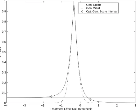
2.1 Confidence curve for a 33 cluster subset of the Epilepsy data. . . 40

2.2 Coverage plots for binomial proportionn=5 . . . 45

(12)

Chapter 1

Generalized Wald, Score, and

Robust Profile Likelihood

Confidence Intervals

1.1 Introduction

In likelihood inference there are three standard methods of generating confidence

in-tervals for a parameter of interest. These three methods are derived by simply inverting the

three corresponding likelihood-based hypothesis tests: the Wald test, the score test, and the

likelihood ratio test. These confidence intervals require that the assumed probability model for

the data is the one that actually generated the data; in other words, the probability model is

not misspecified. If the assumed likelihood is misspecified, then the error rates for these

(13)

These standard intervals rely on the theory which states that Wald, score, and likelihood ratio

tests are all asymptotically distributed as χ2 _{random variables. If the model is incorrect this}

asymptotic result may not hold, often leading to higher than nominal error rates. In the case

of the Wald and score tests, there are relatively simple modifications of the test statistics that

can be made so that the adjusted statistics follow an asymptotic χ2 _{distribution even when}

the assumed model is incorrect. However, in the case of the likelihood ratio test, this is not in

general possible. Under model misspecification, the likelihood ratio test statistic is distributed

asymptotically as a linear combination ofp₋p0χ21random variables (chi-squared with 1 degree

of freedom), where p and p0 are the dimensionalities of the full parameter space and the

pa-rameter space under the null hypothesis, respectively (Kent 1982). The task of finding critical

values for such a distribution is somewhat computationally challenging, and application-level

software to compute such critical values does not appear to be generally available, which is

pos-sibly why it is uncommon to find the likelihood ratio test used in situations where the model

is expected to be incorrect. However, in the case of confidence intervals, we are only interested

in the situation where p₋p0 = 1. The likelihood test then follows the distribution of a χ21

multiplied by a scalar constant that is not difficult to estimate. This fact appears to be quite

unappreciated at this time. It suggests a procedure for generating confidence intervals that is

in many ways superior to robust versions of the Wald and score confidence intervals. In this

chapter we discuss and compare the generalized, robust versions of the Wald, score, and profile

(14)

1.2 Notation

Let the data be denoted byY=_{yi}ni=1, and suppose that the assumed model for the

data is that the individual data points,yi, are independent random variables that have density

yi ∼ f(yi|θ,xi), where θ is an unknown parameter of dimension p, and each xi is a known

vector of covariates whose dimension is less than or equal top. The true density that generated

the complete data Y is g(Y_|θ,X), and is unknown. In particular, g is not necessarily equal to Q

f(yi|θ,xi) for any value of θ. We assume that regularity conditions like those in White

(1982) hold for f(y_|θ,x) and g(Y_|θ,X), so that the maximum likelihood estimator (MLE) of θ under model f, ˆθn, is strongly consistent for θt, the true value of θ, and is asymptotically

normally distributed. The model log likelihood is,

ln(θ|Y) = n

X

i=1

logf(yi|θ,xi). (1.1)

We denote the gradient of the log likelihood, or score function, by,

S(θ) = ∂

∂θln(θ|Y). (1.2)

There are two information-type matrices that will be of use. These are, assuming that the

necessary limits exist,

I(θ) = ₋ lim

n→∞Eg

" 1 n

n

X

i=1

∂2

∂θ∂θT logf(yi|θ,xi)

#

(15)

and,

D(θ) = lim

n_→∞Eg

" 1 n n X i=1 ∂

∂θlogf(yi|θ,xi) ∂

∂θT logf(yi|θ,xi)

#

. (1.4)

Asg is unknown in practical situations, one commonly uses empirical estimators for

the two preceding quantities,

ˆ

I(θ) = ₋1

n

X

i=1

∂2

∂θ∂θT logf(yi|θ,xi), (1.5)

and

ˆ

D(θ) = 1

n

X

i=1

∂

∂θlogf(yi|θ,xi) ∂

∂θT logf(yi|θ,xi). (1.6)

Note that, strictly speaking, these are not truly estimates, but are estimates of a matrix function

that takes θ as its argument.

Because our interest lies in confidence intervals, we partitionθinto

θ =     ψ η     , (1.7)

whereψ is the scalar parameter of interest and η is the vector containing the remaining p₋1 parameters. When vector or matrix quantities are seen with subscripts such as S1 or I12,

we assume that the full vector or matrix has been partitioned conformally with the (ψ, η)

(16)

The restricted MLE ofη under the constraint thatψis held fixed,˜η(ψ), figures

promi-nently in the calculation of generalized score and robust likelihood intervals, and is computed

by solving

S2(ψ,η(ψ)) = 0.˜ (1.8)

1.3 Generalized Wald Confidence Intervals

Because of its simplicity, the generalized Wald confidence interval has been the most

commonly used confidence interval that is robust to misspecification. Once parameter

estima-tion is completed, the generalized Wald interval is not difficult to compute, and has a simple,

easily interpretable, form.

However, there are some serious drawbacks to these intervals. Although under very

broad conditions the generalized Wald interval has an asymptotic coverage rate equal to the

nominal 1₋αrate, in practical small sample situations the actual coverage may be significantly smaller than stated. The generalized Wald interval also lacks the parameterization invariance

that the other two likelihood-based intervals, the generalized score and robust profile likelihood

intervals, often share.

The generalized Wald interval is motivated by the asymptotic normality of the MLE

under possible model misspecification. Under broad conditions, the MLE, ˆθn, has an asymptotic

normal distribution (Stefanski and Boos 2002)

√

(17)

This convergence suggests an obvious form for the generalized Wald statistic for testing

H0:ψ=ψ0,

TGW(ψ0) =

n( ˆψ₋ψ0)2

{Iˆ−1_(ˆ_{θ) ˆ}_D_(ˆ_{θ) ˆ}_I−1_(ˆ_θ)_}₁₁. (1.10)

This generalized Wald test statistic, which has a null asymptotic χ2

1 distribution, is easily

inverted to obtain the corresponding confidence interval,

ˆ ψn±

q

{Iˆ−1_(ˆ_{θ) ˆ}_D(ˆ_{θ) ˆ}_I−1_(ˆ_θ)_} 11

z1₋α/2

√

n , (1.11)

wherez₁₋_α/₂ is the 1₋α/2 quantile of the standard normal distribution. In order to improve the generalized Wald interval’s coverage we will often use critical values from thet-distribution

with n₋p degrees of freedom, which can dramatically improve its small sample performance. We will call such intervals generalized Wald-t confidence intervals.

The quantity ˆI−1_(ˆ_{θ) ˆ}_D(ˆ_{θ) ˆ}_I−1_(ˆ_{θ) is commonly referred to as the}_{sandwich matrix}_{, and}

plays a central role in robust likelihood inference.

1.4 Generalized Score Confidence Intervals

The generalized score interval arises from inverting the generalized score statistic (Boos

1992) for the hypothesisH0: ψ=ψ0,

TGS(ψ0) =n−1ST(˜θ) ˆI−1(˜θ)e1(eT1Iˆ−1(˜θ) ˆD(˜θ) ˆI−1(˜θ)e1)−1eT1Iˆ−1(˜θ)S(˜θ)

=n−1_ST_(˜_{θ) ˆ}_I−1_(˜_θ)S(˜_θ)_· {Iˆ−1(˜θ)}11

{Iˆ−1_(˜_{θ) ˆ}_D(˜_{θ) ˆ}_I−1_(˜_θ)_} 11

,

(18)

where ˜θ= (ψ0,η(ψ˜0))T, ande1 is the unit vector whose first element is one, and the remaining

elements are zero.

The first representation is the form of the fully general, hypothesis via constraint,

version of the generalized score test statistic (Boos 1992), for the special case of H0 :ψ =ψ0.

The second form is reduced from the first and highlights its relationship to Rao’s original

score test statistic, n−1_ST_I−1_{S. The generalized score test statistic is equal to Rao’s score}

test multiplied by a scalar robust correction constant. This form, a non-robust test statistic

multiplied by a robust correction, is similar of the robust likelihood ratio test, that we introduce

in the next section.

In many common situations, the generalized score test is invariant to differentiable

parameter transformations. We are easily able to verify this using an argument similar to one

given in Stafford (1996). A sufficient condition for the generalized score test to be invariant is

that the observed and expected information matrices coincide. This is the case, for example, in

generalized linear models with canonical link function, since the second derivative matrix of the

loglikelihood is functionally independent of Y. Suppose that (ψ, ηT) is an invertible and twice

differentiable reparameterization of (τ, λT_{) = (τ}_{(ψ), λ}T_{(ψ, η)). Notice that the two parameters}

ψandτ are measuring the same quantity on different scales of measurement whose relationship

may be nonlinear. This means that H0 : ψ = ψ0 and H0 : τ =τ(ψ0) are testing the same

hypothesis. If we differentiate the reparameterized likelihood,ln(τ(ψ), λ(ψ, η)|Y), and take the

necessary expectations for the computation of information matrices, we obtain theψ-scale score

vector and information matrices,

(19)

Iψ = J(ψ, η)I(τ(ψ), λ(ψ, η))J(ψ, η)T, (1.14)

and

Dψ = J(ψ, η)D(τ(ψ), λ(ψ, η))J(ψ, η)T, (1.15)

whereJ is the Jacobian of the reparameterization,

J(ψ, η) = 

  

∂τ

∂ψ 0T

∂λ

∂ψ ∂η∂λT



  

. (1.16)

Now, Rao’s score test statistic is invariant because,

(JS)T(JIJT)−1_{(JS) =}_ST_JT_J−T_I−1_J−1_JS

=STI−1_S,

(1.17)

establishes that theψ-scale andτ-scale score test statistics coincide. Partitioned-matrix algebra

shows the invariance of the correction constant, although individually ˆI(θ) and ˆD(θ) are not

invariant.

{J−T_I−1_J−1_}₁₁

{(J−T_I−1_J−1_)(JDJT_)(J−T_I−1_J−1₎_} 11

= {J−

T_I₋1_J₋1_}

11

{J−T_I−1_DI−1_J−T_}

11

= J

2

11{I−1}11

J2

11{I−1DI−1}11

= {I−

1_} 11

{I−1_DI−1_} 11

.

(20)

This demonstrates that the generalized score test statistics in the ψ-scale and theτ-scale have

the same value, proving the invariance of the generalized score test statistic.

If ψ0 is the true value of ψ, then the TGS has an asymptotic χ21 distribution, like

the generalized Wald statistic. This test statistic is derived using the asymptotic distribution

of n−1_{S(θ), which is a mean of independent random variables, and therefore, under broad}

regularity conditions, is asymptotically normally distributed by the Central Limit Theorem.

The Wald statistic also implicitly assumes thatn−1_{S(θ) is normally distributed, but in addition}

requires the use of the delta theorem to obtain the asymptotic normality of ˆθ, as it is the

solution of the equation S( ˆθ) = 0. Thus, one would expect that the χ2₁ approximation to

the distribution of the generalized score statistic would be more accurate than that of the

generalized Wald statistic. The generalized score statistic contains only restricted estimates of

θ under the null hypothesis. This usually gives it a slight computational advantage over the

Wald and likelihood ratio tests, because there is one less parameter that needs to be estimated.

Unfortunately, this computational advantage does not carry over to generalized score confidence

intervals. This is because obtaining the generalized score confidence interval amounts to solving

TGS(ψ)−z12−α= 0 twice: once each for the upper and lower endpoints of the interval. AsTGS

is generally a nonlinear function ofψ, an iterative procedure is required, and ˜η(ψ) will have to

be recomputed during each iteration.

As the simulations later in this chapter show, in small samples the generalized score

confidence intervals maintain their nominal coverage rate better than the generalized Wald

intervals, but in small samples they can be highly inefficient. These confidence intervals can

be many times wider than generalized Wald intervals, and in some situations can be infinite in

(21)

profile likelihood confidence interval.

1.5 Robust Profile Likelihood Confidence Intervals

The robust profile likelihood confidence interval is the least well known of the

likelihood-based intervals, possibly because the critical values of the asymptotic distribution of the robust

likelihood ratio test initially appear to be difficult and unwieldy to compute. A somewhat

closer look reveals that robust likelihood confidence intervals are no more difficult to compute

than generalized score confidence intervals, however. The idea behind these intervals goes back

to Foutz and Srivastava (1977), and Kent (1982), who independently derived the asymptotic

distribution of the likelihood ratio test under model misspecification. Unlike the generalized

Wald and score statistics, except for the scalar parameter of interest case, there is no direct

modification of the likelihood ratio statistic that generally gives it an asymptotic χ2

distribu-tion. In place of such a modification, Foutz et al, and Kent found the asymptotic distribution

of the likelihood ratio test under misspecification. The asymptotic form of the likelihood ratio

statistic for H0:ψ=ψ0, is

2(ln(ˆθ)−ln(ψ0,η(ψ˜ 0)). (1.19)

Assuming for the moment thatψhas dimensionp0 between 1 andp, Kent (1982) gives

the asymptotic distribution of the test statistic to be that of

p0

X

i=1

(22)

where theXi are independentχ21 random variables, and theci are the eigenvalues of the matrix

{{I(θ)−1_}

11}−1{I(θ)−1D(θ)I(θ)−1}11. (1.20)

Finding critical values for a linear combination of χ2 random variables can be done using

Imhof’s algorithm (Imhof 1961), but in the case of confidence intervals, this is unecessary, as

the asymptotic distribution of the likelihood ratio test is just a scalar constant multiplied by a

χ2₁ random variable. This correction constant cis simply the robust estimate of the variance of

ψ divided by the model based variance estimate,

c = {I(θ)−

1_D(θ)I(θ)−1_} 11

{I(θ)−1_} 11

, (1.21)

and can be consistently estimated by simply inserting the MLE of ˆθ,

ˆ

c = {I(ˆθ)−

1_D(ˆ_θ)I(ˆ_θ)−1_} 11

{I(ˆθ)−1_}₁₁ . (1.22)

So, for scalar ψ, the robust likelihood ratio test statistic is defined to be

TRLR(ψ0) =

2(ln(ˆθn)−ln(ψ0,η(ψ˜ 0)))

ˆ

c , (1.23)

and has an asymptotic χ2

1 distribution underH0 :ψ=ψ0.

Like the generalized score interval, the robust profile likelihood interval is invariant

under all differentiable reparameterizations that preserve ψ (Stafford 1996). This is easily

(23)

demonstration of the generalized score test’s invariance, and also by the well-known invariance

of the likelihood ratio test statistic.

The simulations later in this chapter indicate that the robust profile likelihood interval

frequently outperforms both the Wald and generalized score confidence intervals. Its coverage

of the true parameter value is closer to nominal than the Wald interval, while lacking the loss

of efficiency and conservatism of the generalized score interval.

1.6 Numerical Computation of Generalized Score and Robust

Profile Likelihood Confidence Intervals

The computation of the endpoints of profile likelihood and generalized score confidence

intervals, while simple in principle, requires some care to ensure that convergence occurs

when-ever possible. The basic problem is this: given a test statisticT(ψ,η(ψ)) whose null distribution˜

isχ2₁, find two solutions (ψL, ψU) to the scalar equation

T(ψ,η(ψ))˜ ₋z₁2

−α/2 = 0. (1.24)

There are several difficulties that an algorithm for finding (ψL, ψU) must overcome. First and

foremost, the algorithm should employ a root bracketing scheme to ensure that the same root

is not found twice. Root bracketing algorithms maintain a bracket, or interval, that is known

to contain the root of an equation. At every iteration, the bracket’s length is decreased until it

is smaller than some prespecified tolerance. The bisection method is the simplest and most well

(24)

finding an initial bracket for each of the confidence interval’s endpoints is made easier because

we know a priori that ψL _<_{ψ < ψ}ˆ U_{, as all likelihood-based tests accept the null hypothesis,}

H0 : ψ = ˆψ. An initial line search is necessary, however, to completely bracket the root, and

to ensure that both of the two roots exist. Unlike Wald type confidence intervals, generalized

score and robust profile confidence intervals are not necessarily finite in length. In fact, if one

were to speak carefully, one would speak instead of generalized score and likelihood confidence

regions, as opposed to intervals, because the set of values of ψ for which test T accepts the

null hypothesis, _{ψ_|T(ψ,η(ψ))˜ < z₁2

−α/2}, is not guaranteed to be an interval at all, even an

infinite one. However, in the experience of the author, generalized score or profile likelihood

confidence regions that are not intervals (finite or infinite in length) are very rare for most

models. Furthermore, the asymptotic equivalence of the generalized Wald test, the generalized

score, and robust likelihood ratio tests (in the case of a single parameter of interest) ensures

that the probability that these confidence regions are not intervals goes to zero as the sample

size becomes large. A final consideration is a slight preference for derivative-free methods for

obtaining (ψL, ψU). Although the derivative of the profile likelihood is not difficult to derive,

the derivative of the generalized score test involves quantities like vector derivatives of the

inverse of a matrix, a tensor of degree three, which would be convenient to avoid computing

whenever possible.

Brent’s scalar root finding method (Brent 1973) provides a solution that meets all

the demands stated in the preceding paragraph, and is fast. In fact, if the derivative is at

least as difficult to compute as the function whose root is being sought, Brent’s method is even

faster than Newton’s method (Press, Teukolsky, Vetterling, and Flannery 1988). The details of

(25)

constructed combination of bisection, regula falsi, and inverse quadratic interpolation that is

put together in such a way that it converges quickly for well behaved problems, and in most

cases does no worse than bisection on hard problems.

Thus, an effective strategy for computing the endpoints of generalized score and robust

profile likelihood confidence intervals is to first perform a line search to find whereT(ψ,η(ψ))˜ ₋ z2₁

−α/2 changes sign from negative to positive. Without loss of generality, we will discuss the

computation of upper endpoints, as the method for computing lower endpoints is completely

analagous. We know from the outset that T( ˆψ,η( ˆ˜ ψ)) = 0, so that for both endpoints the

side of the root bracket that corresponds to where T(ψ,η(ψ))˜ ₋z2₁

−α/2 < 0 can be initially

set to ˆψ. Then, we initialize ψ to be equal to the upper generalized Wald endpoint and

computeT(ψ,η(ψ))˜ ₋z2

1−α/2. Because of the asymptotic equivalence of these likelihood-based

tests, the generalized Wald upper endpoint makes a perfectly reasonable, easily computed,

starting value. We continue incrementing ψby the standard error of the MLE, and computing

T(ψ,η(ψ))˜ ₋z2₁

−α/2 until this quantity becomes positive. Once this happens, a bracket that

contains the upper endpoint of the confidence interval has been found, and one can now employ

Brent’s method (or bisection, or any other root finding algorithm) to obtain a solution to the

equation. However, if after a predetermined number of steps, a value ofψthat yields a positive

value of T(ψ,η(ψ))˜ ₋z₁2

−α/2 has not been found, declare the endpoint to be infinite in value.

1.7 Simulations

In this section are the results of simulations that compare the generalized Wald,

(26)

logistic and log-linear GEE models, Huber robust linear regression models, and linear

measure-ment error models.

Generalized estimating equations (GEE) models are an important class of models

that extend the applicability of generalized linear models to data that are correlated within

clusters (Liang and Zeger 1986). The standard method for hypothesis testing and generating

confidence intervals for parameters of a GEE model is the generalized Wald test. However, it

is well known (Gunsolley, Getchell, and Chinchilli 1995) that Wald methods do not perform

well in datasets where the number of clusters is small. In this section we give the results from

a number of simulations that provide evidence that the generalized score and robust profile

likelihood confidence intervals offer a significant improvement over the standard generalized

Wald interval. It also becomes clear that the generalized score interval is often less efficient

than the robust profile likelihood interval, as measured by its length.

1.7.1 Logistic Regression GEE

We investigate, via simulation, the small sample properties of confidence intervals for

parameters that describe the mean of binary data that is correlated in clusters. Two situations

are examined. The first is a series of simulations in the case of simple linear logistic regression,

and the second set of simulations are motivated by the data from a study (Preisser and Qaqish

1999) of urinary incontinence.

Simple Linear Logistic GEE Simulations

In each of the following simulations we generateNS = 2000 data sets in the following

(27)

represent the data by _{yij} where i = 1,2, . . . K and j = 1,2,3,4. The data for each cluster

is then created using Al-Osh and Lee’s algorithm for generating correlated binary data, given

a specific mean and correlation structure (Al-Osh and Lee 2001). The observations within the

cluster are individuallyBernoullirandom variables whoselog odds of equalling 1 areη+ψxij,

where the xij are independently drawn U nif orm(−1,1) random variables, and the values η

and ψ are known constants. The observations within the cluster have common correlation, γ,

where the value ofγ is either 0, .2, or .5, depending on the simulation.

We estimateθ= (ψ, η)T with a GEE model using the independence working

correla-tion matrix, that amounts to ordinary simple linear logistic regression using thexijas covariates.

We then use the estimate ofθto form 95% (equal tail) generalized Wald, generalized score, and

robust profile likelihood confidence intervals for ψ. Because of the overall poor performance of

the generalized Wald interval, we also report simulation results for the generalized Wald interval

using t-distribution critical values in place of the more commonly used normal-theory critical

values. By analogy with linear models, the degrees of freedom for the t-distribution critical

values is set to the number of clusters minus the number of estimated parameters. Using these

critical values dramatically improves the coverage of the generalized Wald interval.

The size of these simulations, NS = 2000, was chosen so that for values near .95 the

estimated coverage probabilities should be known to within about .01 of the true value with

95% certainty. The proportion of the confidence intervals that covered the true value of ψ

are reported, along with median length of the intervals. The median length was chosen to be

reported, rather than the mean length, because the possibility of infinite intervals renders the

mean a useless measure of typical length. We also report the proportion of intervals that are

(28)

and is a manifestation of a significant loss of inferential power.

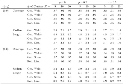
Table 1.1: Coverage and length for generalized Wald, score, and robust likelihood intervals for Bernoulli data under a simple linear logistic regression model.

ρ= 0 ρ= 0.2 ρ= 0.5

(ψ, η) # of ClustersK= 5 10 20 5 10 20 5 10 20

(0,0) Coverage Gen. Wald .87 .92 .93 .85 .92 .93 .82 .91 .93

Gen. Wald-t .96 .94 .94 .97 .93 .95 .94 .95 .95

Gen. Score .98 .96 .95 .98 .96 .95 .98 .95 .94

Rob. Like. .95 .95 .96 .95 .96 .95 .95 .95 .95

Median Gen. Wald 2.9 2.1 1.5 2.9 2.1 1.5 2.7 2.1 1.5

Length Gen. Wald-t 4.8 2.5 1.6 4.8 2.5 1.6 4.5 2.5 1.7

Gen. Score ∞ 3.4 1.8 ∞ 3.4 1.8 ∞ 3.5 1.8

Rob. Like. 3.7 2.4 1.6 3.7 2.4 1.6 3.7 2.4 1.6

Gen. Wald-t .97 .96 .94 .97 .94 .95 .94 .93 .94

Gen. Score .97 .96 .95 .96 .95 .95 .96 .93 .94

Rob. Like. .95 .96 .95 .93 .96 .96 .88 .91 .94

Median Gen. Wald 3.2 2.3 1.6 3.0 2.3 1.6 3.8 3.0 2.2

Length Gen. Wald-t 5.4 2.8 1.7 5.1 2.7 1.7 7.0 3.6 2.3

Gen. Score ∞ 3.8 2.0 ∞ 3.9 1.9 ∞ 5.7 2.7

Rob. Like. 3.9 2.6 1.7 4.0 2.6 1.7 4.9 3.2 2.2

Note: Estimated coverages have approximate standard error (.95)(.05)/2000 =.005. Cluster size=4.

There are two things that are immediately seen by glancing at the simulation results

in Tables 1.1 and 1.2. The first is that the generalized Wald interval’s coverage rate is much too

low. In none of these simulations does the generalized Wald interval’s coverage rate exceed.94,

and in the smallest sample sizes it is below .87. This result is not really surprising, however,

since it is known that Wald tests can perform very poorly in small samples. The second striking

result is the extreme conservatism of the generalized score interval, especially in small samples.

When K = 5 it is generally infinite in length about 90% of the time. However, when the

(29)

Table 1.2: Proportion of infinite length generalized score and robust likelihood intervals for Bernoulli data under simple a linear logistic regression model.

ρ= 0 ρ= 0.2 ρ= 0.5

(ψ, η) # of ClustersK= 5 10 20 5 10 20 5 10 20

(0,0) Proportion Gen. Score .87 .01 0 .90 .01 0 .92 .05 0

Infinite Rob. Like. 0 0 0 0 0 0 .01 0 0

(1,0) Proportion Gen. Score .91 .04 0 .92 .06 0 .96 .16 .01

Infinite Rob. Like. 0 0 0 0 0 0 0 0 0

interval’s, while its coverage is generally lower than that of the robust profile interval’s.

The robust profile likelihood interval and the generalized Wald interval usingtcritical

values perform well, and are quite competitive. Except for the (ψ= 1, ρ=.5) case, the robust

profile likelihood interval maintains its coverage well. The generalized Wald-t interval also

maintains its coverage well, but appears to be less efficient than the robust likelihood interval,

as its median length in these simulations is uniformly longer than the robust profile likelihood’s

in all the K= 5 and K = 10 situations.

GUIDE Data Example and Simulations

The next group of simulations is motivated by the relatively recent Guidelines for

Urinary Incontinence Discussion and Evaluation (GUIDE) study (Preisser and Qaqish 1999).

In this study, researchers contacted 137 patients from 38 medical practices that suffered from

various degrees of incontinence, and were asked whether their incontinence interfered with

their day to day activities, or otherwise bothered them. Their response to this question was

considered to be the independent variable of interest (1=bothered), and there were five other

covariates: a sex indicator (SEX), the scaled and centered ages (AGE), the average number of

(30)

of times per day the patient uses the restroom to urinate (TOILET). The data are assumed

to be correlated within each medical practice. The data from one of the clusters was removed

because of missing values in one of the covariates for all patients in the cluster, leaving a

total of 37 clusters. The cluster sizes ranged from 1 to 8, and an analysis of the data using

a GEE model with the exchangeable working correlation matrix yielded an estimate of the

within-cluster correlation equal to .17.

The data in the simulations were generated in a manner similar to the previous

sim-ulations. We generate simulation data using parameter values equal to the logistic regression

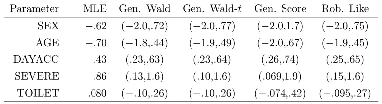
MLE for the complete data set, which are displayed in Table 1.3 with their corresponding 95%

confidence intervals.

Table 1.3: Logistic regression MLE’s and approximate 95% GEE confidence intervals for the GUIDE dataset.

Parameter MLE Gen. Wald Gen. Wald-t Gen. Score Rob. Like SEX ₋.62 (₋2.0,.72) (₋2.0,.77) (₋2.0,1.7) (₋2.0,.75) AGE ₋.70 (₋1.8,.44) (₋1.9,.49) (₋2.0,.67) (₋1.9,.45)

DAYACC .43 (.23,.63) (.23,.64) (.26,.74) (.25,.65)

SEVERE .86 (.13,1.6) (.10,1.6) (.069,1.9) (.15,1.6)

TOILET .080 (₋.10,.26) (₋.10,.26) (₋.074,.42) (₋.095,.27)

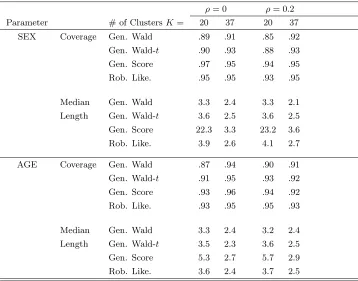
We provide simulation results for confidence intervals about the SEX and AGE

pa-rameters in Tables 1.4 and 1.5. Two sample sizes are investigated, the full dataset (ignoring the

clusters with missing covariate information) of K = 37 clusters, and also a subset of the data

consisting of K = 20 clusters. Two values of the within cluster correlation are investigated,

ρ = 0 and ρ=.2. For these values of the regression parameters, it is not possible to generate

(31)

imposed on the correlation by having different observations within a cluster having different

success probabilities.

Table 1.4: Coverage and length for generalized Wald, score, and robust likelihood intervals for clustered Bernoulli data simulated from the GUIDE dataset.

ρ= 0 ρ= 0.2

Parameter # of ClustersK= 20 37 20 37

SEX Coverage Gen. Wald .89 .91 .85 .92

Gen. Wald-t .90 .93 .88 .93

Gen. Score .97 .95 .94 .95

Rob. Like. .95 .95 .93 .95

Median Gen. Wald 3.3 2.4 3.3 2.1

Length Gen. Wald-t 3.6 2.5 3.6 2.5

Gen. Score 22.3 3.3 23.2 3.6

Rob. Like. 3.9 2.6 4.1 2.7

AGE Coverage Gen. Wald .87 .94 .90 .91

Gen. Wald-t .91 .95 .93 .92

Gen. Score .93 .96 .94 .92

Rob. Like. .93 .95 .95 .93

Median Gen. Wald 3.3 2.4 3.2 2.4

Length Gen. Wald-t 3.5 2.3 3.6 2.5

Gen. Score 5.3 2.7 5.7 2.9

Rob. Like. 3.6 2.4 3.7 2.5

(32)

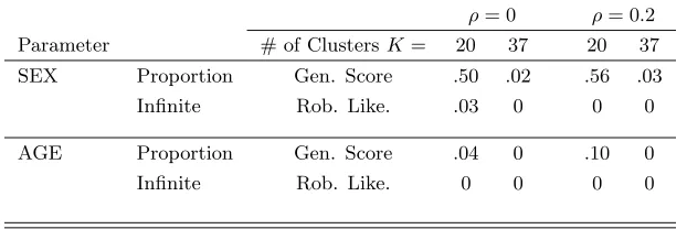
Table 1.5: Proportion of infinite length generalized score and robust likelihood intervals for clustered Bernoulli data simulated from the GUIDE dataset.

ρ= 0 ρ= 0.2

Parameter # of ClustersK= 20 37 20 37

SEX Proportion Gen. Score .50 .02 .56 .03

Infinite Rob. Like. .03 0 0 0

AGE Proportion Gen. Score .04 0 .10 0

Infinite Rob. Like. 0 0 0 0

In these simulations the difference in the performances of the generalized Wald-t and

robust profile intervals is more pronounced. Here the robust profile interval clearly outperforms

the other confidence intervals. Again we see the inefficiency of the generalized score interval.

When K= 20 the generalized score interval for the SEX effect was infinite 50% of the time.

1.7.2 Poisson Regression GEE

As in the previous section, we provide simulation results from two groups of

simula-tions. The first group of simulation results is from simple linear Poisson regression where the

data are correlated in clusters, and the second group is motivated by the data from a study of

epileptic seizures (Thall and Vail 1990).

Simple Linear Poisson GEE Simulations

Like the logistic regression simulations we generate NS = 2000 datasets for each

simulation. For each dataset there are a total of K clusters of size 4, where K is 10, 20 or

50. We represent the data by _{yij} wherei = 1,2, . . . K and j = 1,2,3,4. To investigate the

(33)

random samples using the algorithm described in Appendix A, which generates autocorrelated

Poisson-type random variates.

We estimateθ= (ψ, η)T with a GEE model using the independence working

correla-tion matrix, essentially fitting a simple linear Poisson regression using thexijas covariates. We

then use the estimate ofθto form the 95% generalized Wald, the generalized Wald-t, generalized

score, and robust profile likelihood confidence intervals forψ. The results of these simulations

(34)

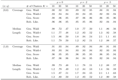
Table 1.6: Coverage and length for generalized Wald, score, and robust likelihood intervals for serially correlated Poisson data under a log linear regression model.

ρ= 0 ρ=.2 ρ=.5

(ψ, η) # of ClustersK= 10 20 50 10 20 50 10 20 50

Gen. Wald-t .93 .94 .94 .93 .94 .95 .92 .93 .94

Gen. Score .98 .96 .95 .97 .96 .96 .96 .95 .96

Rob. Like. .96 .96 .95 .95 .95 .96 .92 .94 .94

Median Gen. Wald .98 .72 .47 1.0 .77 .50 1.1 .86 .56

Length Gen. Wald-t 1.1 .77 .48 1.2 .83 .52 1.3 .92 .58

Gen. Score 1.5 .86 .50 1.8 .94 .54 2.1 1.1 .61

Rob. Like. 1.1 .79 .50 1.2 .82 .51 1.2 .88 .57

Gen. Wald-t .93 .93 .94 .93 .93 .94 .92 .93 .93

Gen. Score .96 .95 .95 .96 .95 .95 .96 .95 .94

Rob. Like. .97 .96 .96 .94 .94 .95 .92 .94 .94

Median Gen. Wald .99 .73 .48 1.1 .78 .51 1.2 .88 .57

Length Gen. Wald-t 1.2 .79 .49 1.2 .84 .53 1.4 .94 .59

Gen. Score 1.5 .87 .51 1.7 .94 .55 2.1 1.1 .63

Rob. Like. 1.2 .80 .50 1.2 .83 .52 1.2 .90 .58

(35)

Table 1.7: Proportion of infinite length generalized score and robust likelihood intervals for serially correlated Poisson data under a log linear regression model.

ρ= 0 ρ=.2 ρ=.5

(ψ, η) # of ClustersK= 10 20 50 10 20 50 10 20 50

(0,0) Proportion Gen. Score .01 0 0 .01 0 0 .06 0 0

(1,0) Proportion Gen. Score 0 0 0 .03 0 0 .05 0 0

The results of these simulations are quite clear. The generalized Wald interval, using

normal critical values performs quite poorly when the sample size is small, and is improved

significantly by the use oft-critical values. In this set of simulations, the robust profile interval

performs reasonably well, except when the sample size is small and the autocorrelation high.

The generalized score interval consistently has good coverage as well, but is somewhat inefficient

relative to the robust profile likelihood, and is occasionally infinite when the sample size is

K = 10, while no infinite length robust profile intervals were observed.

Epilepsy Data Example and Simulations

The data in the following example comes from a study of the effect of the anti-seizure

drug, progabide, on epileptics (Thall and Vail 1990). In this experiment 59 patients were

randomized into treatment and placebo (standard chemotherapy) groups. A baseline two-week

count of seizures was recorded for the period before treatment was begun, and four other seizure

counts were recorded for each patient at intervals of two weeks over the course of the eight-week

study. Parameter estimates were obtained by fitting a Poisson regression model using treatment

(TREATMENT), age (AGE), and an indicator of baseline vs. study period seizure count as

(36)

intervals are given in Table 1.8.

Table 1.8: Poisson regression MLE’s and approximate 95% GEE confidence intervals for the Epilepsy dataset.

Parameter MLE Gen. Wald Gen. Wald-t Gen. Score Rob. Like

TREATMENT ₋0.8 (₋.76,.59) (₋.78,.60) (₋1.0,.58) (₋.77,.60) AGE ₋.44 (₋1.4,.49) (₋1.4,.51) (₋1.5,.86) (₋1.4,.46) BASELINE ₋1.3 (₋1.6,₋.97) (₋1.6,₋.97) (₋1.7,₋.99) (₋1.6,₋.98)

In the following simulations, we used a method analogous to the simple linear Poisson

GEE simulations, using the same method to generate counts that are serially correlated within

a patient. The simulated data were generated using the correlated parameter values equal to

the study data’s MLE. In each simulation, 2000 simulation replications of the data were created.

Two sample sizes were used, the full set of 59 observations, and a subset of 30 patients with 15

(37)

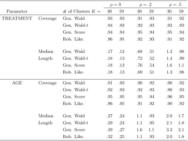
Table 1.9: Coverage and length for generalized Wald, score, and robust likelihood intervals for serially correlated Poisson data using the Epilepsy data covariates and MLE.

ρ= 0 ρ=.2 ρ=.5

Parameter # of ClustersK= 30 59 30 59 30 59

TREATMENT Coverage Gen. Wald .93 .93 .91 .93 .91 .92

Gen. Wald-t .94 .93 .92 .93 .92 .93

Gen. Score .94 .94 .95 .94 .95 .94

Rob. Like. .96 .95 .92 .93 .91 .92

Median Gen. Wald .17 .12 .68 .51 1.3 .98

Length Gen. Wald-t .18 .13 .72 .52 1.4 .99

Gen. Score .18 .13 .76 .54 1.6 1.1

Rob. Like. .18 .13 .69 .51 1.3 .98

AGE Coverage Gen. Wald .91 .93 .90 .92 .90 .92

Gen. Wald-t .92 .93 .92 .93 .90 .93

Gen. Score .95 .95 .95 .94 .96 .95

Rob. Like. .96 .95 .91 .92 .90 .92

Median Gen. Wald .27 .24 1.1 .93 2.0 1.7

Length Gen. Wald-t .29 .24 1.1 .95 2.1 1.8

Gen. Score .39 .27 1.6 1.1 3.2 2.1

Rob. Like. .32 .25 1.1 .93 2.0 1.8

Note: Estimated coverages have approximate standard error (.95)(.05)/2000 =.005. Cluster size=5. Less than .005 of each of the intervals were reported as infinite.

The simulation results are consistent with the simple linear Poisson GEE simulations.

The generalized score interval maintains its coverage better than the other intervals, especially

as the within cluster correlation becomes larger. No infinite length generalized score intervals

were observed. These observations lead us to recommend that the generalized score confidence

interval be used in the analysis of correlated Poisson-type data.

1.7.3 Huber Robust Linear Regression

We investigate the performance of these confidence intervals for robust linear regression

(38)

xT_i β+i, where the’s are iid with median 0, but are not assumed to be normally distributed.

β = (β1, β2) has dimension p, andβ1 is the scalar parameter of interest. Parameter estimation

of the mean parameters,β, proceeds by solving,

n

X

i=1

ψ yi−x

T

i βˆ

σ !

xi = 0, (1.25)

where Huber’sψ-function is given by,

ψ(z) =       

z if_|z_|< k k_·sign(z) otherwise.

(1.26)

For all of the simulations in this study, we usek = 1. Solving the above estimating equation is

equivalent to maximum likelihood estimation, where the density of the errors has the functional

form exp(₋ρ(z)/σ), where ρ(z) is defined to be,

ρ(z) =        z2

2 if|z| < k

k_|z_{| −} k₂2 otherwise.

(1.27)

We estimate the scale parameter,σ, by solving

n

X

i=1

χ(yi−x

T

i β

ˆ

σ )−(n−p)EΦ(χ) = 0 (1.28)

whereχ(z) =zψ(z)₋ρ(z), andEΦ represents expectation with respect to the standard normal

distribution.

Unlike the previous simulations, we do not compute a restricted estimate of σ while

(39)

simulations indicated that these confidence intervals suffered a loss of efficiency when this was

done. However, restricted estimates of β₂ are computed.

Robust likelihood ratio tests of ANOVA models using Huber’sψ-function were

inves-tigated by (Schrader and Hettmansperger 1980). In their paper, Schrader and Hettmansperger

develop a modeling strategy completely analogous to standard least squares ANOVA using

ro-bust likelihood ratio tests. Although they describe a complete system for likelihood testing of

robust linear models, I have not seen their approach generalized to interval estimation.

Their approach differs, somewhat, from the one we used for GEE models, however.

Rather than use the purely empirical estimators for I and D,

ˆ σ n n X i=1

ψ0 yi−xTi βˆ

ˆ σ

!

xixTi ,

and ˆ σ n n X i=1

ψ2 yi−x

T

i βˆ

ˆ σ

!

xixTi ,

respectively, they use estimates ofIandDthat assume that the data are identically distributed,

ˆ σ n n X i=1

ψ0 yi−x

T

i βˆ

ˆ σ

! _n X

i=1

xixTi ,

and ˆ σ n n X i=1

ψ2 yi−x

T

i βˆ

ˆ σ

! _n X

i=1

xixTi ,

(40)

consistent estimator for the likelihood ratio test’s robust correction constant is

ˆ

cψ = ξ

n n₋p

Pn

i=1ψ2

y(i)−xTiβˆ

ˆ

σ

Pn

i=1ψ0

y(i)₋xTiβˆ

ˆ

σ

,

whereξ is a bias correction that is given by,

ξ= 1 + p n

n₋Pn

i=1ψ0

_y i−xTiβˆ

ˆ

σ

Pn

i=1ψ0

yi−xTiβˆ

ˆ

σ

.

Taking the analogy with ANOVA further, they use theF distribution as the reference

distribution for the robust likelihood ratio test instead of the χ2 distribution.

Schrader and Hettmansperger also investigate a bias corrected version of the

gener-alized Wald test statistic that, like their version of the robust likelihood ratio test, assumes

that the data are iid. Inverting this generalized Wald test yields a bias corrected version of the

generalized Wald interval,

ˆ

β1±tn₋p(1−α/2)

ˆ σ √ n v u u u t n n₋pξ

Pn

i=1ψ2(

yi−xTiβˆ

ˆ

σ )

(Pn

i=1ψ0(

yi−xTiβˆ

ˆ

σ ))2

(XT_X₎−1 1,1.

Like their robust likelihood ratio test, Schrader and Hettmansperger use a t distribution to

obtain critical values for the Wald test.

In each of the simulations below, we report coverages and median lengths for 5 types

of confidence intervals: the ordinary least squares t confidence interval (OLSt), the

Schrader-Hettmansperger generalized Wald interval (SH-Gen. Wald) and the Schrader Hettmanperger

(41)

score and robust profile likelihood intervals.

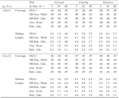
In each simulation we generateN = 2000 datasets from the modelyi =µ+βxi+ei,

i= 1,2, . . . n, where n is equal to 10, 20, or 50, and the xi are equally spaced in the interval

(₋1,1). In the first group of simulations β = µ = 0, and the ei’s are iid, but are generated

from one of three distributions: N ormal(0,1), Cauchy, or a mixture distribution where each

ei has a 75% probability of coming from aN ormal(0,1) distribution, and a 25% probability of

being aCauchy random variate. In this way, we can see the loss of efficiency when the data are

normally distributed, and compare the performance of the various confidence intervals when

the data are heavy tailed, or prone to outliers.

For the second group of simulations β = µ = 1, and the ei’s are independent, but

no longer identically distributed. This allows us to determine whether or not the performance

of the Schrader-Hettmansperger intervals is sensitive to the assumption that the errors are

iid. Here the ei are distributed as either a N ormal(0,1), a Cauchy, or a 75%-25% mixture

of the two, multiplied by a scale parameter, σi, that varies with the xi’s according to the rule

σi =.1 +|µ+xiβ|. Tables 1.10 and 1.11 show the results of these simulations.

As measured by coverage, all the confidence intervals perform quite well, with

cov-erages often at or exceeding 95% in most of the simulations. We are therefore compelled to

make our recommendation based on the lengths of the intervals. As one would expect, the

OLS tinterval performs the best when the error are iid from a N ormal(0,1) distribution, but

is inefficient when the distribution of the errors has heavy tails. Like the previous simulations,

the generalized score interval is often inefficient when the sample size is small, and is

occasion-ally infinite in length. The robust profile likelihood interval (the general version that does not

(42)

The Schrader and Hettmansperger (SH) version of the robust likelihood interval is the most

efficient, and maintains its coverage well, even when the errors are not iid. The SH-robust

profile interval is generally shorter than the SH-generalized Wald interval, and is the one we

(43)

Table 1.10: Coverage and length for generalized Wald, score, and robust likelihood intervals for iid data under a simple linear Huber regression model.

Dist. N ormal Cauchy M ixture

(µ, β, σ) # Obs. K= 5 10 20 5 10 20 5 10 20

(0,0,1) Coverage OLSt .94 .94 .95 .97 .96 .96 .96 .97 .96

SH-Gen. Wald .93 .94 .95 .96 .96 .95 .96 .95 .95

SH-Rob. Like. .93 .94 .95 .96 .95 .95 .96 .96 .95

Gen. Score .95 .95 .95 .97 .95 .95 .96 .96 .95

Rob. Like. .95 .96 .98 .97 .97 .97 .97 .95 .97

Median OLS-t 2.1 1.5 .94 8.1 7.8 7.9 6.2 6.1 5.7

Length SH-Gen. Wald 2.3 1.6 1.0 4.7 3.0 1.7 3.6 2.3 1.4

SH-Rob. Like. 2.2 1.5 .99 4.6 2.9 1.7 3.5 2.2 1.3

Gen. Score 2.7 1.6 1.0 8.4 3.6 1.8 6.6 2.8 1.4

Rob. Like. 2.4 1.8 1.1 4.9 3.2 1.9 3.8 2.5 1.5

(1,1,σ†_i) Coverage OLSt .95 .94 .95 .97 .97 .97 .96 .96 .97

SH-Gen. Wald .95 .95 .95 .97 .95 .95 .95 .95 .94

SH-Rob. Like. .94 .95 .95 .96 .95 .95 .95 .95 .94

Gen. Score .95 .94 .95 .96 .94 .94 .95 .97 .95

Rob. Like. .95 .96 .97 .97 .97 .97 .95 .94 .97

Median OLS-t 2.3 1.6 1.0 8.1 8.3 8.4 2.9 2.4 2.2

Length SH-Gen. Wald 2.3 1.6 1.0 4.6 2.9 1.7 2.5 1.7 1.0

SH-Rob. Like. 2.2 1.6 .98 4.5 2.8 1.7 2.4 1.6 1.0

Gen. Score 2.2 1.7 1.0 8.1 3.5 1.8 3.4 1.8 1.1

Rob. Like. 2.4 1.7 1.1 4.6 3.1 1.9 2.6 1.8 1.1

Note: Estimated coverages have approximate standard error.005. †_σ

i=.1 +|µ+xi|.

Table 1.11: Proportion of infinite length generalized score and robust likelihood intervals for iid data under a simple linear Huber regression model.

Dist. N ormal Cauchy M ixture

(µ, β, σ) # of ObsK= 10 20 50 10 20 50 10 20 50

(0,0,1) Proportion Gen. Score .01 0 0 .12 .01 0 .12 0 0

(44)

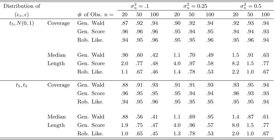
1.7.4 Simple Linear Regression With Covariate Measurement Error

We investigate the performance of the generalized Wald, generalized score, and

ro-bust profile likelihood confidence intervals in the context of simple linear measurement error

models. In these models we assume that the data consist of pairs (y, u) where y is the

in-dependent random variable of interest, and u plays the role of the covariate. In addition, it

is assumed, however, that there is an unobserved random variable, x, such that x =µx+x

where x ∼ N ormal(0, σ2x). The observed variables, y and u, are assumed to have model,

y = µ+βx+ and u = x+u, where and u are independent of one another, as well as

with x, and normally distributed, each with mean 0, and variances σ2 and σu2, respectively.

Unfortunately this model is not completely identified, which means that one cannot estimate

all six parameters, (µ, β, µx, σ2, σ2x, σu2). To circumvent this difficulty we assume that the

mea-surement error variance, σ2

u, is known a priori. We form the likelihood-based on the model

described above and use it to find global and restricted estimates of the parameters.

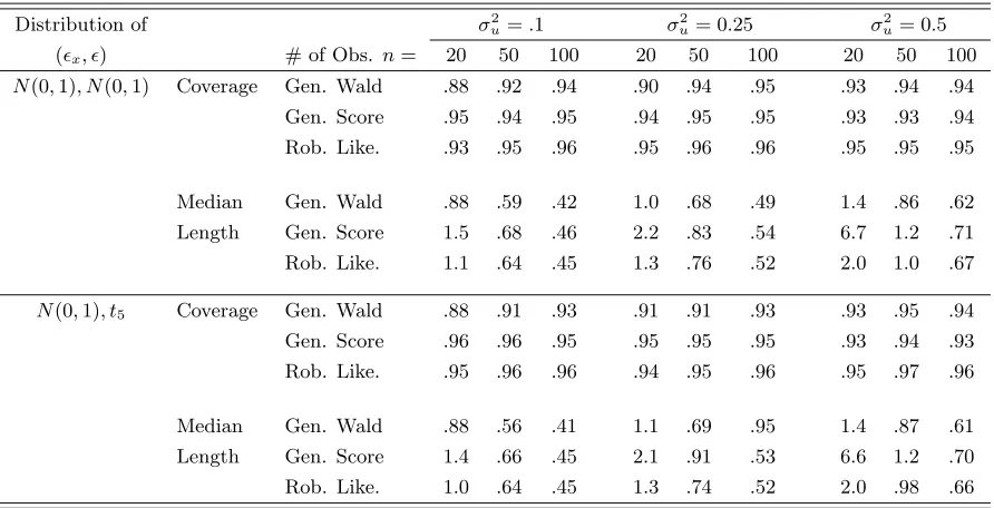
To examine the effects of model misspecification we examine four situations. In each

of these the identified scale parameters satisfyσ2 ₌_σ2

x= 1, and the distributions ofandxare

either N ormal(0,1), or scaled t5 so that the error variance is 1. The mean model parameters

have true values, µ = µx = 0, and β = 1. The measurement error variance, σu2 is varied,

taking on values .1, .25, and .5. We provide simulation results for all four possible combinations

of N(0,1) and t5 distributions for and x. Three sample sizes are investigated, n = 20,50,

and 100. In each simulation, NS=2000 independent samples are drawn, and for each the 95%

generalized Wald, generalized score and robust profile likelihood confidence intervals for the

(45)

interval is created using t critical values with n₋2 degrees of freedom, but the generalized score and robust profile likelihood confidence intervals simply use χ2

1 critical values. Tables

1.12, 1.13, and 1.14 below contain the results of these simulations.

Table 1.12: Coverage and length for generalized Wald, score, and robust likelihood intervals from simple linear measurement error model.

Distribution of σ2

u=.1 σu2 = 0.25 σ2u= 0.5

(x, ) # of Obs. n= 20 50 100 20 50 100 20 50 100

N(0,1), N(0,1) Coverage Gen. Wald .88 .92 .94 .90 .94 .95 .93 .94 .94

Gen. Score .95 .94 .95 .94 .95 .95 .93 .93 .94

Rob. Like. .93 .95 .96 .95 .96 .96 .95 .95 .95

Median Gen. Wald .88 .59 .42 1.0 .68 .49 1.4 .86 .62

Length Gen. Score 1.5 .68 .46 2.2 .83 .54 6.7 1.2 .71

Rob. Like. 1.1 .64 .45 1.3 .76 .52 2.0 1.0 .67

N(0,1), t5 Coverage Gen. Wald .88 .91 .93 .91 .91 .93 .93 .95 .94

Gen. Score .96 .96 .95 .95 .95 .95 .93 .94 .93

Rob. Like. .95 .96 .96 .94 .95 .96 .95 .97 .96

Median Gen. Wald .88 .56 .41 1.1 .69 .95 1.4 .87 .61

Length Gen. Score 1.4 .66 .45 2.1 .91 .53 6.6 1.2 .70

Rob. Like. 1.0 .64 .45 1.3 .74 .52 2.0 .98 .66

Note: Estimated coverages have approximate standard error (.95)(.05)/2000 =.005.

Here we see that the generalized Wald confidence interval is liberal, while the

gener-alized score interval is quite inefficient, and in some circumstances it is frequently infinite in

length. The robust profile likelihood confidence interval performs well, as measured its coverage

(46)

Table 1.13: Coverage and length for generalized Wald, score, and robust likelihood intervals from simple linear measurement error model.

Distribution of σ2

u=.1 σ2u= 0.25 σ2u= 0.5

(x, ) # of Obs. n= 20 50 100 20 50 100 20 50 100

t5, N(0,1) Coverage Gen. Wald .87 .92 .94 .90 .92 .94 .92 .93 .94

Gen. Score .96 .96 .96 .95 .94 .95 .94 .94 .93

Rob. Like. .94 .95 .96 .95 .95 .96 .95 .96 .94

Median Gen. Wald .90 .60 .42 1.1 .70 .49 1.5 .91 .63

Length Gen. Score 2.0 .77 .48 4.0 .97 .58 8.2 1.5 .77

Rob. Like. 1.1 .67 .46 1.4 .78 .53 2.2 1.0 .67

t5, t5 Coverage Gen. Wald .88 .91 .93 .91 .91 .93 .93 .95 .94

Gen. Score .96 .95 .95 .95 .94 .94 .96 .93 .93

Rob. Like. .94 .95 .96 .95 .95 .95 .95 .95 .94

Median Gen. Wald .88 .56 .41 1.1 .69 .95 1.4 .87 .61

Length Gen. Score 1.9 .75 .47 4.0 .96 .57 8.0 1.5 .77

Rob. Like. 1.0 .65 .45 1.3 .78 .53 2.0 1.0 .67

Note: Estimated coverages have approximate standard error (.95)(.05)/2000 =.005.

Table 1.14: Proportion of infinite length generalized score and robust likelihood intervals from simple linear measurement error model.

Distribution of σ2

u=.1 σ2u= 0.25 σ2u= 0.5

(x, ) # of Obs. n= 20 50 100 20 50 100 20 50 100

N(0,1), N(0,1) Proportion Gen. Score .05 0 0 .06 0 0 .12 0 0

Infinite Rob. Like. 0 0 0 0 0 0 .05 0 0

N(0,1), t5 Proportion Gen. Score .04 0 0 .07 0 0 .15 0 0

Infinite Rob. Like. 0 0 0 .01 0 0 .05 0 0

t5, N(0,1) Proportion Gen. Score .18 .03 .01 .21 .02 .01 .22 .05 0

t5, t5 Proportion Gen. Score .17 .02 .01 .20 .03 .01 .23 .05 .01

(47)

Chapter 2

Length-Optimal Interval Estimation

In this chapter we introduce a general procedure for taking an existing confidence

in-terval procedure and creating a new one. We call this new confidence inin-terval procedure

length-optimal interval estimation, as it finds the shortest asymptotically level-α confidence interval

in an infinite class of asymptotically level-α confidence intervals. Some theory is developed for

the case of the single parameter likelihood intervals that demonstrates that the length-optimal

profile likelihood intervals are asymptotically equivalent to the more common equal-tail

likeli-hood interval, indicating that the length-optimal intervals retain their asymptotic error rate of

1₋α. Simulation results are provided that show that in some circumstances the small sample coverage rate of these confidence intervals is higher than their standard counterparts.

2.1 Motivation and Description

In the previous chapter, we saw that the generalized score interval often has superior

(48)

How-ever, the generalized score interval was observed to be inefficient, and in some circumstances

suffered from the defect of being infinite in length a significant proportion of the time.

Length-optimal confidence interval procedures were motivated by an attempt to correct these problems

of the generalized score interval. As we shall see, the length-optimal approach is only modestly

successful in reducing the conservatism of the generalized score interval, but when we apply

the procedure to the robust profile likelihood and generalized score intervals in simulations we

see the surprising result that the length-optimal versions of the intervals often enjoy higher

coverage than their equal-tail counterparts.

Confidence intervals are generally formed by inverting a two-sided level-α hypothesis

test. That is, the endpoints of the confidence interval are found by inverting two level-α/2

one-sided hypothesis tests, H0 : ψ ≤ ψ0, and H0 : ψ ≥ ψ0. Since the error rate is allocated

equally to each side, such intervals are sometimes called equal-tail confidence intervals. For a

given test statistic, T(ψ0), with an asymptotic χ21 distribution, the endpoints of the equal-tail

confidence interval, (ψL, ψU), are obtained by solving T(ψL) =z_α/2 ₂ and T(ψU) =z_α/2 ₂ subject

to the constraint thatψL<ψ < ψˆ U. When one or more of these two equations has no solution,

the confidence interval will have infinite length. This occurs when, for instance, for all ψ0<ψˆ

the value of the test statistic never exceedsz_α/2 ₂, or, equivalently, the p-value of the hypothesis

test never drops belowα/2.

To remedy this situation, we can reallocate the error rate of the confidence intervals

by introducing a new parameter, , that takes on values in (0,1). Rather than place an error

rate of α/2 to each side of the interval, we can distributeα to the lower side of the interval,

Model-Robust Interval Estimation

Contents

List of Tables

List of Figures

Chapter 1

Generalized Wald, Score, and

Robust Profile Likelihood

Confidence Intervals

1.1

Introduction

1.2

Notation

1.3

Generalized Wald Confidence Intervals

1.4

Generalized Score Confidence Intervals

1.5

Robust Profile Likelihood Confidence Intervals

1.6

Numerical Computation of Generalized Score and Robust

Profile Likelihood Confidence Intervals

1.7

Simulations

Chapter 2

Length-Optimal Interval Estimation

2.1

Motivation and Description