HE, YUN. Multiscale Signal Processing and Shape Analysis for an Inverse SAR
Imaging System. (Under the direction of Prof. Hamid Krim.)
The great challenge in signal processing is to devise computationally efficient and statisti-cally optimal algorithms for estimating signals from noisy background and understanding their contents. This thesis treats the problem of multiscale signal processing and shape analysis for an Inverse Synthetic Aperture Radar (ISAR) imaging system. To address some of the limita-tions of conventional techniques in radar image processing, an information theoretic approach for target motion estimation is first proposed. A wavelet based multiscale method for shape enhancement is subsequently derived and followed by a regression technique for shape recog-nition.
Building on entropy-based divergence measures which have shown promising results in many areas of engineering and image processing, we introduce in this thesis a new generalized divergence measure, namely the Jensen-R´enyi divergence. Upon establishing its properties such as convexity and its upper bound etc., we apply it to image registration for ISAR focusing as well as related problems in data fusion.
Attempting to extend current approaches to signal estimation in a wavelet framework, which have generally relied on the assumption of normally distributed perturbations, we pro-pose a novel non-linear filtering technique, as a pre-processing step for the shapes obtained from an ISAR imaging system. The key idea is to project a noisy shape onto a wavelet domain and to suppress wavelet coefficients by a mask derived from curvature extrema in its scale space representation. For a piecewise smooth signal, it can be shown that filtering by this curvature mask is equivalent to preserving the signal pointwise H ¨older exponents at the singular points, and to lifting its smoothness at all the remaining points.
MULTISCALE SIGNAL PROCESSING AND SHAPE ANALYSIS
FOR AN INVERSE SAR IMAGING SYSTEM
by
YUN HE
A dissertation submitted to the Graduate Faculty of North Carolina State University
in partial fulfillment of the requirements for the degree of
Doctor of Philosophy
ELECTRICAL ENGINEERING
Raleigh June, 2001
APPROVED BY:
Professor Hamid Krim Professor Brian L. Hughes
Chair of Advisory Committee
iii
Biography
Acknowledgments
This endeavor was truly a learning experience. Thanks are due to many people for their interactions and collaborations.
I consider it a privilege to have worked under the supervision of Professor Hamid Krim, and owe him a great deal for his guidance, patience, and financial support through generous grants from Air Force Office of Scientific Research (AFOSR) and Multidisci-plinary University Research Initiative (MURI). I have benefited immensely from his insight, wisdom, suggestions, comments, and constructive criticism of my work. I es-pecially thank him for teaching me how to see the “big picture” as related to my re-search.
I would also like to thank my committee members Professor Brian L. Hughes and Professor Alexandra Duel-Hallen for their expertise and advice. I learned the funda-mentals of communication and information theory through their classes and seminars. Their way of teaching showed me an excellent example of a systematic and straightfor-ward fashion in presenting technical ideas. I am also grateful to have Professor Siamak Khorram on my thesis committee board. I thank him for his inquisitive comments and numerous suggestions in accuracy assessment, which led to many improvements in this thesis.
I also want to thank Dr. Victor Chen from Naval Research Laboratory for providing me the experimental data; and numerous developers of WaveLab, which is a Matlab toolbox freely available over the Internet. Without WaveLab, I guess I would have to spend at least one more year developing all the software.
It was a great pleasure to have closely worked with Dr. A. Ben Hamza and Dr. Yufang Bao. As coworkers, I thank them for the numerous suggestions, guidance, com-ments, and heated, friendly and enlightening discussions. I also want to thank my fellow graduate students for being good officemates, especially Oleg Poliannikov, for sharing coke and sense of humor which made many tough moments so brief.
pa-v tience and kind help in numerous paperwork, travel arrangement and equipment or-ders. She is really a life saver.
Contents
List of Tables xi
List of Figures xiii
1 Introduction 1
1.1 Problem Motivation and Formulation . . . 2
1.2 Thesis Organization and Main Contributions . . . 7
2 Inverse SAR Imaging System 11 2.1 Range Processing . . . 12
2.2 Cross-Range Processing . . . 14
2.3 Maximum Integration Angle . . . 15
2.4 Range Doppler Imaging . . . 17
3 Inverse SAR Image Registration 21 3.1 Introduction . . . 21
3.2 Problem Statement . . . 24
3.4 The Jensen–R´enyi Divergence: Performance Bounds . . . 30
3.5 Image Registration with the Jensen-R´enyi Divergence . . . 32
3.5.1 Discussion . . . 36
3.6 Numerical Experiments: ISAR Image Registration . . . 37
3.7 Conclusions . . . 42
3.8 Appendix . . . 43
4 Introduction to Multiscale Analysis 47 4.1 Multiscale Approximation ofL 2 (R) . . . 47
4.2 Orthonormal Wavelet Basis . . . 51
4.3 Fast Orthogonal Wavelet Transform . . . 58
4.4 Filter Banks and Biorthogonal Wavelets . . . 61
4.4.1 Perfect Reconstruction Filter Banks . . . 62
4.4.2 Biorthogonal Wavelets . . . 64
4.4.3 Lifting Wavelets . . . 68
4.5 Separable Wavelet Bases . . . 71
4.6 Signal Estimation in Wavelet Framework . . . 76
5 Multiscale Signal Enhancement 85 5.1 Introduction . . . 86
5.2 Regularity measurement with wavelets . . . 88
5.3 Problem Formulation . . . 89
5.4 Curve evolution and singularity detection . . . 91
5.5 A smoothness constrained filter . . . 94
5.6 Numerical Experiments . . . 99
5.7 Conclusion . . . 105
5.8 Appendix . . . 106
6 Multiscale Image Fusion 111 6.1 Introduction . . . 111
ix
6.3 Problem Formulation . . . 117
6.4 Image Fusion with Jensen-R´enyi divergence . . . 119
6.4.1 Multi-Sensor Image Fusion . . . 120
6.4.2 Multi-Modality Image Fusion . . . 121
6.4.3 Multi-Spectral Image Fusion . . . 121
6.4.4 Multi-Focus Image Fusion . . . 122
6.4.5 Performance Measures . . . 122
6.5 Conclusion . . . 124
7 Shape Recognition 131 7.1 Shape Space and Shape Distance . . . 132
7.2 Euclidean Shape Matching . . . 135
7.3 Affine Shape Matching . . . 137
7.4 Estimation by Matching . . . 138
8 Conclusions and Discussions 143 8.1 Conclusions . . . 143
8.2 Suggestions for future research . . . 145
List of Tables
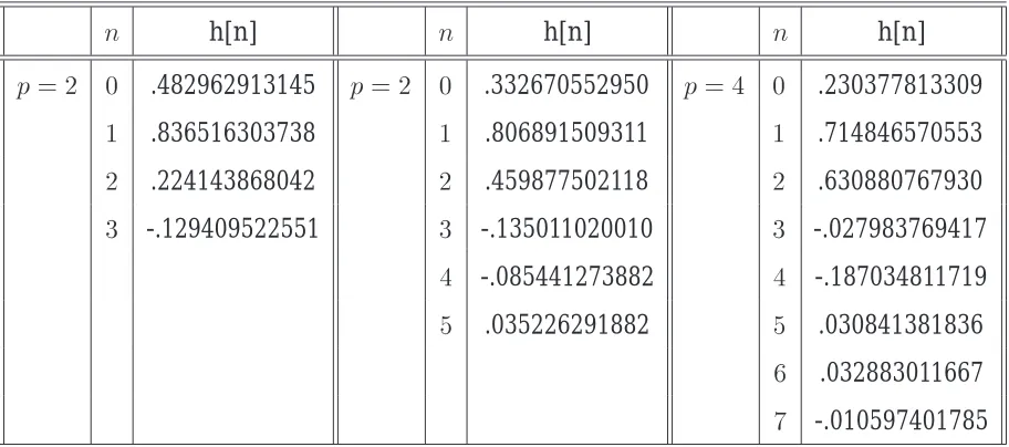
4.1 Daubechies filter coefficients for wavelets withp=2;3;4vanishing
mo-ments. . . 55 4.2 Perfect reconstruction filters h and
~
h for compactly supported spline
biorthogonal wavelets withpandp~vanishing moments. . . 66
6.1 Correlations between different fusion results and source images . . . 123 6.2 Standard deviation between an ideal image and fusion results by
differ-ent algorithms. . . 124 7.1 Symmetric discrepancy measures between the target and aircraft
tem-plates. . . 137 7.2 Shape distances between the estimated mean shape and templates in the
database . . . 141 7.3 Shape distances between noisy configurations to the B-52 template. . . . 141
List of Figures
2.1 Spotlight SAR . . . 11
2.2 SAR/ISAR equivalence . . . 12
2.3 Simplified Geometry for Range Processing . . . 14
2.4 Cross Range Processing . . . 15
2.5 Unfocused ISAR geometry . . . 16
2.6 ISAR Imaging System Architecture . . . 18
2.7 ISAR Image of A Small Boat . . . 19
3.1 Shannon and R´enyi entropy of Bernoulli distribution p = (p;1 p) for different values of. . . 26
3.2 3D representation of Jensen-R´enyi divergenceJR ! (p;q),p = (p;1 p), q =(q;1 q),=0:7,! =(0:5;0:5). . . 27
3.3 Jensen-R´enyi divergence as a function of . . . 30
3.4 Conditional probability distributions . . . 32
3.5 Mutual information vs. Jensen-R´enyi divergence of uniform weights . . 33
3.6 Registration result in the presence of the noise . . . 35
3.7 Effect of the orderin image registration . . . 36
3.9 Polar formatted data in spatial frequency space . . . 38
3.10 ISAR Image of Moving Target . . . 40
3.11 Trajectory of a MIG-25 during imaging time . . . 41
3.12 Image registration of a MIG-25 Trajectory . . . 42
3.13 Reconstructed MIG-25 by polar reformatting . . . 43
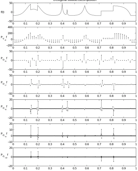
4.1 Orthogonal wavelet decomposition at different scales . . . 53
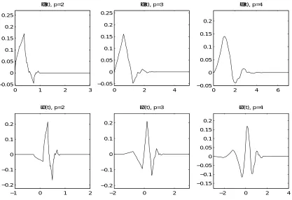
4.2 Daubechies scaling function and wavelets . . . 56
4.3 Symmlet scaling functions and wavelets . . . 57
4.4 Fast Wavelet transform calculation by conjugate mirror filters . . . 60
4.5 A two channel perfect reconstruction filter banks . . . 62
4.6 Spline biorthogonal scaling functions and wavelets for(p=2;p~=4)and (p=3;p~=7) . . . 67
4.7 The biorthogonal filter banks with a lifting and a dual lifting . . . 69
4.8 Wavelet decomposition of a toolbox image . . . 73
4.9 Two-dimensional fast wavelet transform calculated by conjugate mirror filters . . . 75
4.10 Estimation by a soft threshold estimator with the SURE thresholdT . . . 83
5.1 A geometric curve flow . . . 92
5.2 Singularity Detection by Curve Evolution . . . 94
5.3 Clean signals, Blocks, Bumps, HeaviSine and Doppler . . . . 95
5.4 Noisy version of Blocks, Bumps, HeaviSine and Doppler . . . . 96
5.5 Denoising results by SureShrink . . . 97
5.6 Multiscale curvature mask for Blocks, Bumps, HeaviSine and Doppler . . . 98
5.7 Filtering results by the smoothness constrained filter . . . 99
5.8 H ¨older exponents adjustment by the smoothness constrained filter . . . 100
xv 5.11 Denoising results by SureShrink for Laplacian noise corrupted signals . 103
5.12 Smoothness constrained filter applied for shapes . . . 104
5.13 Denoising results by the smoothness-constrained filter . . . 110
6.1 A general framework for multiscale fusion with wavelet transform . . . 112
6.2 Two-dimensional fast biorthogonal wavelet transform calculated by per-fect reconstruction filter banks . . . 116
6.3 Experiment on Multi-sensor image fusion . . . 126
6.4 Experiment on Multi-modality image fusion . . . 127
6.5 Experiment on Multi-spectral remote sensing image fusion . . . 128
6.6 Experiment on Multi-focus image fusion . . . 129
7.1 A shape database in experiment . . . 136
7.2 A set of 16 noisy observation of a B-52 shape . . . 140
CHAPTER
1
Introduction
I
NVERSE Synthetic Aperture Radar (ISAR) is an imaging technique that achieves a
high resolution by exploiting the relative motion between a stationary radar and
a moving target. This is accomplished by coherently processing the returned radar
signals so as to synthesize the effect of a larger aperture array laid out along the target’s
path of motion. One important application of ISAR is as a front-end system for the
purpose of target recognition. The fundamental goal is to detect and recognize objects
of interest in a noisy environment.
A typical ISAR imaging system consists of image acquisition, data fusion, target shape
extraction and enhancement, and finally shape recognition. The main theme of this
thesis is focused on information theoretic imaging and shape analysis. An information
theoretic approach for ISAR image focusing and fusion is first proposed to serve as
a robust stage for image acquisition. A wavelet based multiscale method for shape
enhancement is subsequently derived to estimate a shape in a noisy background which
is followed by a regression technique for shape recognition.
1.1
Problem Motivation and Formulation
Motivated by the current limitations of conventional techniques in radar image focus-ing, target shape estimation and recognition, this thesis addresses the following issues.
Information theoretic approach for ISAR image focusing
The ISAR imagery is induced by the target rotation, which in turn causes time varying spectra of the reflected signals and blurs the resulting image. When a target exhibits complex motion, such as rotation and maneuvering, a standard motion compensation is not adequate to generate an acceptable image for viewing and analysis. In this thesis, we tackle this problem by an information theoretic approach.
In the work of Woods [1] and Viola [2], mutual information, a basic concept from in-formation theory, is introduced as a measure of evaluating the similarity between im-ages. When the two images are properly matched, corresponding areas overlap, and the resulting joint histogram contains high values for the pixel combinations of the corresponding regions. When the images are mis-registered, non-matched areas also overlap and will contribute to additional pixel combinations in the joint histogram. In case of misregistration, the joint histogram has less significant peaks and is more dis-persed than that of the correct alignment of images. The registration criterion is hence to find a transformation such that the mutual information of the corresponding pixel pair intensity values in the matching images is maximized. This approach is accepted widely [3] as one of the most accurate and robust registration measures. Following the same argument, Hero [4] et al. extends the concept to apply R´enyi entropy to measure the joint histogram as a dissimilarity metric between images.
1.1. PROBLEM MOTIVATION AND FORMULATION 3
The objective of ISAR image registration is to estimate the target motion during the imaging time. Let T
(l ;;) be a Euclidean transformation with translational parameter l = (l
x ;l
y
), rotational parameter and scaling parameter . Given two ISAR image
framesf 1 and
f
2, the estimates of target motion parameters (l
;
;
)are given by (l
;
;
)=argmax (l ;;)
D JR
!
(f 1
;T (l ;;)
f 2
) (1.1)
where D JR
!
()is an induced similarity measure based on the proposed Jensen-R´enyi
divergence of orderand weight!, which is maximal whenf
1matches T
(l ;;) f
2. As the
radar tracks the target, the reflected signal is continuously recorded during the imaging time. By registering a sequence of consecutive image frames,ff
i g
N
i=0, the target motion
during the imaging time can be estimated by interpolatingf(l i
; i
; i
)g N
i=1. Based on the
estimated trajectory of the target, translational motion compensation (TMC), and rota-tional motion compensation (RMC) [6] can be used to generate a focused image of the target.
Multiscale Signal Enhancement: Beyond the Normality and Independence
As-sumption
To fulfill the goal of an ISAR imaging system of recognizing objects of interest in a noisy environment, shape enhancement is required and constitutes a crucial step. Donoho and Johnstone [7] first showed that effective noise suppression may be achieved by wavelet shrinkage, in comparison to traditional linear methods. Given the noisy wavelet coefficients, i.e. the true wavelet coefficients plus a noise term, and assuming that one has knowledge of the true wavelet coefficients, an ideal filter sets a noisy coefficient to zero if the noise variance
2
is greater than the square of the true wavelet coefficient; otherwise the noisy coefficient is kept. In this way, the mean square error of this ideal estimator is the minimum of
2
and the square of the coefficient. Under the assumption of i.i.d. normal noise, it can shown that a soft thresholding estimator achieves a risk at mostO(logM)times the risk of this ideal estimator, whereM is the length of the
obser-vation.
approach to characterize the signal, and they proved that the estimation risk is close to the minimax risk by setting a threshold
T = p
2log e
M:
Krim and Pesquet [8] have given an alternative derivation for this threshold, using Rissanen’s Minimum Description Length (MDL) criterion [9] and the assumption of normally distributed noise. The threshold T increase with M is due to the tail of the
Gaussian distribution, which tends to generate larger noise coefficients when sample size increases. This threshold is not optimal, and in general a lower threshold reduces the risk. To refine the threshold, a SureShrink [10] procedure is proposed. Sureshrink calculates thresholds by the principle of minimizing the Stein unbiased estimate of risk for threshold estimates. SureShrink is also based on the assumption of i.i.d. normal noise, which does not hold for ISAR applications. For non-Gaussian type of noise, Neumann [11], Averkamp and Houdre [12] studied the choice of thresholds by having recourse to asymptotics. Wavelet thresholding theory is, however, based on the as-sumption that we know the statistics of the noise to determine an adequate threshold. This makes the algorithm less flexible and less adaptive to different scenarios which can result in an even worse reconstruction. Compensation for the lack of a prior knowledge of the noise statistics may be handled by adopting the minimax principle [13] upon de-riving the worst case noise distribution.
Points of sharp variations are often among the most important features for analyzing properties of transient piecewise smooth signals. To characterize the singular struc-tures, H ¨older exponents [14] provide a pointwise measure of a function over a time interval. Due to the pioneering work by Jaffard [15] and Meyer [16], it can be shown that a local signal singularity of a function is characterized by the decay of its wavelet transform amplitude across scales.
1.1. PROBLEM MOTIVATION AND FORMULATION 5
problem as one of carefully controlling the H ¨older exponents of measured data with a goal of extracting the signal portion with some smoothness fidelity to the original. Let
f 2L 2
(R). We consider an additive noise model. The measured data are
Z(t)=f(t)+N(t); (1.2)
where the noise is modeled by the realization of a zero mean random process N.
De-note f
() and N
()characterize the pointwise H ¨older exponent of f() and N()
re-spectively. A ideal operatorT satisfies the following two conditions: !
^
f =TZ admits f
()as its pointwise H ¨older exponent !V(t)=Z(t)
^
f(t)admits N
()as its pointwise H ¨older exponent
This non-linear filter is optimal in the sense of recovering the smoothness of the true underlying signal.
Information theoretic approach for multiscale image fusion
With the development of new imaging sensors arises the need for image processing techniques that can effectively fuse images from different sensors into a single coherent composition for interpretation. In order to make use of inherent redundancy and ex-tended coverage of multiple sensors, we propose a multiscale approach for pixel level image fusion. The ultimate goal is to reduce human/machine error in detection and recognition of objects.
Over the past two decades, a wide variety of pixel-level image fusion algorithms has been developed. These techniques may be classified into linear superposition, logical filter [17], mathematical morphology [18], image algebra [19] [20], artificial neural net-work [21], and simulated annealing [22] methods. Each of these algorithms focuses on the fact that the fused image reveals new information concerning features that can not be perceived in individual sensor images. However, some useful information has been discarded since each fusion scheme tends to emphasize different attributes of the im-age. Luo [23] provides a detailed review of these techniques.
method which is widely accepted [24] as one of the most effective techniques for image fusion. Wavelet theory has played a particularly important role in multiscale analysis. A number of papers [25] [26] [27] have addressed fusion algorithms based on the or-thogonal wavelet transform. A major drawback in the recent pursuit of wavelet-based fusion algorithms is due to a lack of a good fusion scheme. Most fusion rules so far proposed are in essence more or less similar to “choose max” scheme proposed by Burt [28], which introduces a significant amount of high frequency noise due to the sudden switch of the fused wavelet coefficient to that which is maximum of the source. This high frequency noise is particularly undesirable to visual perception.
In this thesis, we apply a biorthogonal wavelet transform to the pixel level image fu-sion. It is possible to construct smooth biorthogonal wavelets of compact support which are either symmetric or antisymmetric. At the exception of a Haar wavelet, it has been shown [29] that symmetric orthogonal wavelets are impossible to construct. Symmetric or antisymmetric wavelets are synthesized with perfect reconstruction fil-ters having a linear phase. This is a desirable property for image fusion applications. Unlike the “choose max” type of selection rules, we propose an information theoretic fusion scheme. For each pixel in a source image, a vector consisting of wavelet coef-ficients at that pixel position across scales is formed to indicate the “activity” of that pixel. We denote these indicator vectors of all the pixels in a source image as its activ-ity map. To make a reasonable comparison among activactiv-ity indicator vectors, we apply our newly proposed divergence measure, Jensen-R´enyi divergence, which is defined in terms of R´enyi entropy.
Letf 1
;f 2
;:::;f n
: Z 2
! R be digital images of the same scene taken from different
sen-sors. Denote
Wf i
=fd 1 i
(j;n);d 2 i
(j;n);d 3 i
(j;n);a i
(L;n)g
0<jL;n2Z
2; i=1;2;:::n
as a biorthogonal wavelet image representation off
i. Our fusion scheme cab be
formu-lated as the following optimization problem:
Wf =arg min Wf2F
8 < :
n X
i=1 (
L X
j=1 X
2 j
n2D0
jWf(j;n) Wf i
(j;n)j 2
) L X
j=1 X
2 j
n2D1
jWf(j;n)j 2
1.2. THESIS ORGANIZATION AND MAIN CONTRIBUTIONS 7
whereD
0is the set of pixels whose activity patterns are similar in all the source images,
whileD
1 is the set of pixels whose activity patterns are different.
F is the set of all the
imagesf whose wavelet transform satisfies
min(Wf i
(j;n)) Wf(j;n)max(Wf i
(j;n));
for any0<j Landn2Z 2
. This constraint makes sure that the solution stays in the closure ofF, i.e., no image outside the scenario we are contemplating.
Shape recognition
The geometrical description of an object can be decomposed into registration and shape information. For example, an object’s location, rotation and size could be the registra-tion informaregistra-tion and the geometrical informaregistra-tion that remains is the shape of the object. An object’s shape is invariant under registration transformations and two objects have the same shape if they can be registered to match exactly.
The pioneers of this topic of general shape and registration analysis are Kendall [30] and Bookstein [31]. Some reference and reviews include Goodall [32], Kent [33], Dry-den and Mardia [34].
The difficulty of target recognition in ISAR imagery is to identify a target shape in the presence of interference regardless of its position, scale and orientation. In an effort to overcome this difficulty, we describe matching of two configurations in Euclidean and affine shape spaces using regression techniques, and we further address robustness is-sues and matching by estimation.
1.2
Thesis Organization and Main Contributions
Chapter 2. Inverse Synthetic Aperture Radar Imaging System
Inverse Synthetic Aperture Radar System transmits electro-magnetic waves to a target and coherently integrates the returned signals to synthesize the effect of a larger aper-ture array. The spatial distribution of the reflectivity density of a target, referred to as the image of the target, is usually mapped onto a range-azimuth plain. In this chapter, we briefly introduce the range and azimuth processing, and necessary procedures to construct an ISAR image from reflected and measured signals.
Chapter 3. Inverse SAR Image Registration: An Information Theoretic Approach
In this chapter, a new generalized divergence measure, Jensen-R´enyi divergence, is pro-posed. Some properties such as convexity and its upper bound are derived. Based on the Jensen-R´enyi divergence, we propose a new approach to the problem of ISAR image registration. Our approach applies Jensen-R´enyi divergence to measure the statistical dependence between consecutive ISAR image frames, which would be maximal if the images are geometrically aligned. Simulation results demonstrate that the proposed method is efficient and effective in tracking the trajectory of a target. The major results of this chapter have been published in [35], [36] and [37].
Chapter 4. Introduction to Multiscale Analysis
In this chapter, we briefly review the concept of multiscale analysis. We study the prop-erties of an operator which approximates a signal at a given resolution. We show that the difference of a signal at different resolutions can be extracted by decomposing the signal on a wavelet orthonormal basis. The development of orthonormal wavelet bases has opened a new bridge between approximation theory and signal processing. In the last section of this chapter, we discuss a hard/soft threshold estimator and SureShrink in particular detail, and illustrate its adaptivity to unknown smoothness via wavelet shrinkage.
Chapter 5. Multiscale Signal Enhancement: Beyond the Normality and
Indepen-dence Assumption
1.2. THESIS ORGANIZATION AND MAIN CONTRIBUTIONS 9
perturbations. In practice, this assumption is often violated and sometimes, even the prior information of a probability distribution of the noise process is unavailable. To relax this assumption, we propose a novel non-linear filtering technique in this chapter. The key idea is to project a noisy signal onto a wavelet domain and to suppress wavelet coefficients by a mask derived from its curvature extrema in a scale space representa-tion. For a piecewise smooth signal, it can be shown that filtering by this curvature mask is equivalent to preserving the signal pointwise H ¨older exponents at the singular points and lifting its smoothness at all the remaining points. The major results of this chapter have been published in [38] and [39].
Chapter 6. A Multiscale Approach for Pixel Level Image Fusion
Pixel level image fusion refers to the processing and synergistic combination of infor-mation gathered by various imaging sources to provide a better understanding of a scene. We formulate the image fusion as an optimization problem and propose an in-formation theoretic approach in a multiscale framework to solve it. A biorthogonal wavelet transform of each source image is first calculated, and the new fusion algo-rithm applies Jensen-R´enyi divergence to construct a composite of wavelet coefficients according to the measurement of the information patterns inherent in source images. Experimental results on fusion of multi-sensor navigation images, multi-modality med-ical images, multi-spectral remote sensing images, and multi-focus optmed-ical images are presented to illustrate the proposed fusion scheme. The major results of this chapter have been published in [40].
Chapter 7. Shape Recognition
Chapter 8. Conclusions and Discussions
CHAPTER
2
Inverse
Synthetic
Aperture Radar
Imag-ing System
Ψ
Target Area
Synthetic Aperture Size
Figure 2.1: Spotlight SAR
I
NVERSE Synthetic Aperture Radar (ISAR) is a microwave imaging system capable of producing high resolution imagery from data collected by a relatively small an-tenna. ISAR can be explained in terms of spotlight SAR [6], as illustrated in Figure (2.1). Spotlight SAR is obtained as the radar antenna constantly tracks a particular target area of interest. The same data would be collected if the radar were stationary and the target area were rotating. The target rotation relative to the radar is used to generate the target image. This is precisely the idea of ISAR.
Figure (2.2) illustrates the data collection from an air target by a stationary radar as
Ψ
R
Rotating Target Moving Radar Stationary Target
Stationary Radar
-L/2 L/2
Ψ R
(a) (b)
Figure 2.2: SAR/ISAR Equivalence: (a) ISAR; (b) SAR equivalence
the target rotates through an angle . The spotlight SAR equivalent geometry is the moving radar of Figure (2.2b), collecting the same data while flying a circular segment around an identical but non-rotating target. The SAR aperture lengthLin Figure (2.2b)
corresponds to integration angle in figure (2.2a).
2.1
Range Processing
ISAR imagery represents reflectivity magnitude associated with the illuminated target. In the terminology of radar signal processing, the direction of radar Line of Sight (LOS) is referred to as range and the direction orthogonal to range is referred to as cross-range or azimuth.
Range is determined by measuring the time it takes for a transmitted signal to travel a round-trip distance between radar and target. The ability of the radar to determine the range of a particular scatterer in a vicinity of other scatterers depends on the range resolution.
2.1. RANGE PROCESSING 13
range of radar viewing angles.
Consider the simplified geometry shown in Figure (2.3). An antenna located at the ori-gin illuminates a line of scatterers centered atx = R, having length W and reflectivity q : R ! C. Let the transmitted signals(t)~ be a pulse of durationT
p and bandwidth
given by
~
s(t)=Refs(t)e j2f
0 t
gw( t T p
) (2.1)
wheres(t)is the baseband equivalent signal of~s(t), and
w(t)= 8 < :
1; jtj 1 2 0; otherwise:
(2.2)
Then, ignoring the round-trip attenuation, the returned signal can be represented as the convolution of target reflectivity density with the transmitted signal
r(x)=q(x)?s(2x=c) (2.3)
wherecis the speed of light, and2x=cis the round trip delay.
An estimate of the reflectivity density can be obtained by passingr(x)through a matched
filter whose impulse response ish r
(x)=s
( 2x=c). Therefore, the estimate ofq(x)is ^
q(x) = r(x)?s
( 2x=c)
= q(x)?[s(2x=c)?s
( 2x=c)]: (2.4)
Let’s define
(t)=s(t)?s
( t) (2.5)
then we can rewrite (2.4) as
^
q(x)=q(x)?(2x=c) (2.6)
Since the transmitted pulse usually has a large time-bandwidth product, (t)can be
approximated by a sinc()function. The estimate of target reflectivity density may thus
be represented as
^
R-W/2 R+W/2 q(x)
x Antenna
R
Figure 2.3: Simplified geometry for range processing.
The range resolution is hence given by [41]
Ær= c 2
: (2.8)
2.2
Cross-Range Processing
To gain a basic understanding of the cross-range resolving mechanism in ISAR, let’s consider Figure (2.4) with a line of scatterers having the reflectivityq(y). As the radar
is moving fromz = L=2toz =L=2, the two-way phase advance at cross-rangeyis
y (z)
4
dr= 4
zsin (2.9)
For the case ofy RandL R, sin approachesy=Randz approachesR ; =2 < < =2, Equation (2.9) can be re-expressed in terms of angle
y ()
4
R y R
= 4
y;
2
<< 2
: (2.10)
Then, the echo response from the line scatterers atis given by
g()= Z
+1
1
q(y)e j
4
y
dy: (2.11)
2.3. MAXIMUM INTEGRATION ANGLE 15
z y
Antenna L/2
-L/2
x
Ψ
dr
R
q (y)
γ
Figure 2.4: Simplified geometry for cross-range processing
over a small integration angle ,
^ q(y) =
Z +
2
2
g()e j
4
y d
= Z
+1
1
g()w(
)e j
4
y d
= q(y)?sinc( 2
y); (2.12)
wherew()is the window function defined in equation (2.2). Therefore the cross-range
resolution is given by [6]
Ær c
= 2
: (2.13)
2.3
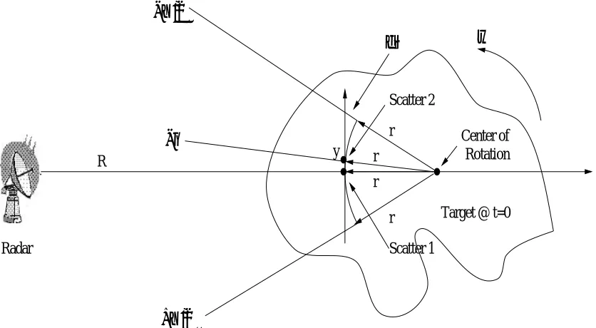
Maximum Integration Angle
r r r
r
Center of Rotation
δ
rTarget @ t=0 Scatter 2
Scatter 1 R
Radar
−Ψ/2
+Ψ/2
ω
−θ
y
Figure 2.5: Unfocused ISAR geometry
during rotation. As in Figure (2.5), for a small ,
r 2
+( r
2 )
2
=(r+Ær) 2
(2.14)
Solving for withr>>Ær, we have
=( 8Ær
r )
1=2
(2.15)
Assume a maximum allowable two-way phase deviation of=8as a criterion for focus,
the corresponding allowable range deviation Ær is =32. The maximum integration
angle [6] then becomes
max =
1 2
r r
: (2.16)
The cross-range resolution in unfocused ISAR is limited by the maximum integration angle max, and a Focused Aperture ISAR is desirable for a larger integration angle. Let’s
consider the echo signal from scatterer 1, located at (r; = 0)when t = 0as shown in
Figure (2.5), the phase advance term at timetis
1 (t)=
4 Ær =
4(!rt) 2
2.4. RANGE DOPPLER IMAGING 17
where the target rotates at a constant angular rotation rate !. The two way phase
ad-vance for scatterer 2, which is located at(r; )whent=0, is
2 (t)=
4
(!t ) 2
r 2
: (2.18)
A focused aperture for ISAR is achieved by subtracting 1
(t)from 2
(t), and we have
y (t)=
2 (t)
1 (t)=
4
[ !ty+ y
2 2r
] (2.19)
where y = r. Define the target rotation angle = !t, then we can rewrite Equation
(2.19) in terms of,
y ()=
4
[ y+ y
2 2r
] (2.20)
Equating (2.20) with (2.11), we obtain the range resolution [6]
Ær c
= 1 2
!T
: (2.21)
where T is the integration time. Equation (2.21) for focused ISAR with !T = is
the same as the cross-range resolution (2.13) for an unfocused, small integration angle ISAR.
The ISAR imaging is induced by target motion. During the imaging time, the scatterers must remain in their range cells. Reflectivity density function won’t remain the same over a wide range of radar viewing angles. Therefore we can not use an arbitrary large integration angle in Equation (2.21). Optimal Integration Angle [35] need to be estimated to achieve the highest possible cross-range resolution and prevent defocusing in the image.
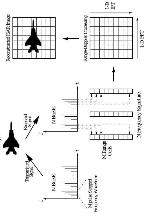
2.4
Range Doppler Imaging
f
t
N Bursts
IFT
t
f
N Bursts
1-D
...
1-D FFT
Reconstructed ISAR Image Range-Doppler Processing
M pulse Stepped
...
M Range Cells
N Frequency Signature
Transmitted
Frequency Waveform
Received Signal
Signal
Target
Figure 2.6: ISAR imaging system architecture
SF waveforms, a radar typically transmits a sequence ofN bursts. Each burst consists
ofM narrow-band pulses. Within each burst, the center frequency of each successive
pulse is increased by a constant frequency stepf. The total bandwidth of the burst,
i.e., =Mf, determines the radar range resolution. The total number of bursts for a
given imaging time determines the Doppler or cross-range resolution.
To form a radar image, N bursts of returned signals first pass through a quadrature
demodulator to obtain in-phase and quadrature signals at baseband. AnM N array
of complex data, fG m;n
g
0mM 1;0nN 1, is constructed to represent an unprocessed
compensa-2.4. RANGE DOPPLER IMAGING 19
Figure 2.7: ISAR Image of A Small Boat
tion. Range compression functions as a matched filter to resolve range. For SF signals, the range compression performs anM-point IFT to each of the N received frequency
signatures
r=F 1 m
(G) (2.22)
whereF 1
m denotes the IFT operation with respect to variable
m. All together,N range
profiles, each containing M range cells, are thus obtained.
Along each range cell, N range profiles constitute a time history series of the target.
The Fourier imaging approach applies a FFT to the time history series and generates a
N-point Doppler spectrum, or Doppler profile. By combining theN Doppler spectra at M range cells, aM N image is formed
I =F n
(r) (2.23)
where F
n denotes a FFT operation with respect to variable
n. The radar image I is
CHAPTER
3
Inverse
SAR
Image
Registration:
An
In-formation
Theoretic
Approach
E
NTROPY based divergence measures have shown promising results in many
ar-eas of engineering and image processing. In this paper, a new generalized
di-vergence measure, Jensen-R´enyi didi-vergence, is proposed. Some properties such as
con-vexity and its upper bound are derived. Based on the Jensen-R´enyi divergence, we
propose a new approach to the problem of ISAR (Inverse Synthetic Aperture Radar)
image registration. The goal of ISAR image registration is to estimate the target motion
during the imaging time. Our approach applies Jensen-R´enyi divergence to measure
the statistical dependence between consecutive ISAR image frames, which would be
maximal if the images are geometrically aligned. Simulation results demonstrate that
the proposed method is efficient and effective.
3.1
Introduction
Image registration is an important problem in computer vision [42] [43], remote
sens-ing data processsens-ing [44] [45] and medical image analysis [46] [47]. The goal of image
registration is to find a spatial transformation such that a similarity metric achieves its
maximum between two or more images taken at different times, from different sensors,
or from different viewpoints.
One such example which is the primary interest in the sequel is Inverse Synthetic Aper-ture Radar (ISAR) imaging. ISAR is a microwave imaging system capable of producing high resolution imagery from data collected by a relatively small antenna. ISAR imag-ing is induced by target motion, which unfortunately also blurs the resultimag-ing image. After a conventional ISAR translational focusing process, image registration can be ap-plied to estimate the target rotational motion parameter, upon which polar re-formating may be used to achieve a higher resolution image. Related work in this area includes the image registration in interferometric SAR processing by Gabriel [48], Li [49] and Lin [50] and Fornaro [51].
Over the last three decades, a wide variety of registration techniques have been devel-oped for different applications. These techniques can be classified [52] into correlation methods, Fourier methods, landmark mapping, and elastic model-based matching. Given two images f
1 ;f
2
: I I 2 R 2
! R, correlation methods [53] calculate the
normalized two-dimensional cross-correlation functionC(f 1
;T (l ;;)
f 2
)betweenf 1 and f
2, where
T is a Euclidean transformation with translational parameterl=(l x
;l y
),
rota-tional parameterand scaling parameter. The registration problem may be succinctly
stated as
(l
;
;
)=argmax l ;;
C(f 1
;T (l ;;)
f 2
): (3.1)
The correlation methods are generally limited to registration problems in which the image is misaligned by only a small rigid transformation. In addition, the peak of the correlation may not be clearly discernible in the presence of noise. Fourier methods [54] are the frequency domain equivalent of the correlation methods. Fourier methods make use of the translation property of the Fourier transform and search for the optimal spec-trum matching between two images. Since rotation is invariant under a Fourier trans-formation, rotating an image merely rotates the Fourier transform of that image [55]. If we denoteF
1 ;F
2 as the two-dimensional Fourier transform of f
1 ;f
2 respectively, we
obtain the phase of the cross-power spectrum rotated by as
P
(! x
;! y
)= F
1 (!
x ;!
y )T
F
2 (!
x ;!
y ) jF (! ;! )T F (! ;! )j
3.1. INTRODUCTION 23
To determine the rotational parameter, one proceeds to maximize the two-dimensional
inverse Fourier transformation ofP
(! x
;! y
), i.e., a cross-correlation which is as peaked
or as impulsive as possible, and the location of that impulse is exactly the translational parameterl. In light of their equivalence to the correlation methods, Fourier methods
are also limited to registration problems with a small rigid transformation. If there exists spatially local variation, then both the correlation methods and the Fourier meth-ods would fail. For cases of unknown misalignment type, landmark mapping tech-niques [56] and elastic model-based matching [57] [58] may be used to tackle the regis-tration problem. Landmark mapping techniques extract feature points from a reference image and a target image respectively, then apply piecewise interpolation to compute a transformation to map the feature point sets from the reference image to the target image. Landmark based methods are usually labor intensive and their accuracy de-pends on the degree of reliability of the feature points. Instead of finding the mapping between the feature point sets, elastic model-based matching methods model the dis-tortion in the image as the deformation of an elastic material. The resulting registration transformation is the deformation with a minimal bending and stretching energy. Prac-tical elastic model-based methods [59] are based on computation expensive iterative algorithms, and the choice of feature points plays a crucial role in its performance.
same argument, Hero [4] et al. extends the concept to apply R´enyi entropy to measure the joint histogram as a dissimilarity metric between images.
Inspired by this previous work, and looking to address their limitation in often dif-ficult imagery, we introduce in this chapter a novel generalized information theoretic measure, namely the Jensen-R´enyi divergence and defined in terms of R´enyi entropy [5]. Jensen-R´enyi divergence is defined as a similarity measurement among any finite number of weighted probability distributions. Shannon mutual information is a special case of the Jensen-R´enyi divergence. This generalization provides us an ability to con-trol the measurement sensitivity of the joint histogram, to ultimately result in a better registration accuracy.
In the next section, we give a brief statement of the problem. In section 3.3, we in-troduce the Jensen-R´enyi divergence and its properties. In Section 3.4, we derive the performance upper bounds of the Jensen-R´enyi divergence in terms of the Bayes error and also of the asymptotic error of the Nearest Neighbor Classifier. Section 3.5 describes the concepts of image registration with the Jensen-R´enyi divergence. Numerical exper-iments for ISAR image registration is demonstrated in Section 3.6. Finally, we provide concluding remarks in Section 3.7.
3.2
Problem Statement
ISAR imagery is induced by target motion, and the target motion in turn causes time-varying spectra of the received signals. Motion compensation has to be applied to obtain a high resolution image. The objective of ISAR image registration is to estimate the target motion during the imaging time. Let T
(l ;;) be a Euclidean transformation
with translational parameterl = (l x
;l y
), rotational parameter and scaling parameter . Given two ISAR image framesf
1 and f
2, the estimates of target motion parameters (l
;
;
)are given by (l
;
;
)=argmaxD JR
!
(f 1
;T (l ;;)
f 2
3.3. THE JENSEN-R ´ENYI DIVERGENCE 25
where D JR
!
()is an induced similarity measure based on Jensen-R´enyi divergence of
orderand weight!, which is maximal whenf
1matches T
(l ;;) f
2. As the radar tracks
the target, the reflected signal is continuously recorded during the imaging time. By registering a sequence of consecutive image frames, ff
i g
N
i=0, the target motion during
the imaging time can be estimated by interpolating f(l i ; i ; i )g N
i=1. Based on the
esti-mated trajectory of the target, translational motion compensation (TMC), and rotational motion compensation (RMC) [6] can be used to generate a focused image of the target.
3.3 The Jensen-R´enyi Divergence
Let k 2 N and X = fx 1
;x 2
;:::;x k
g be a finite set with a probability distribution p = (p
1 ;p
2 ;:::;p
k ), i.e.
P k j=1
p j
=1andp j
=P(x j
)0, whereP()denotes the probability.
R´enyi entropy is a generalization of Shannon entropy [60], and is defined as
R (p)= 1 1 log k X j=1 p j
; >0 and 6=1: (3.4)
For>1, the R´enyi entropy is neither concave nor convex.
For 2 (0;1), it is easy to see that R´enyi entropy is concave, and tends to Shannon
entropyH(p)as ! 1. It can easily be verified thatR
is a non-increasing function of , and hence
R
(p)H(p); 82(0;1): (3.5)
In the sequel, we will restrict 2(0;1), unless otherwise specified, and will use a base 2logarithm, i.e., the measurement unit is bits.
As shown in Figure 3.1, uncertainty is at a minimum when Shannon entropy is used, and it increases asdecreases. R´enyi entropy attains a maximum uncertainty when
is equal to zero.
Definition 3.1 Letp 1
;p 2
;:::;p nbe
nprobability distributions onX and!=(!
1 ;! 2 ;:::;! n )
be a weight vector such that P
n !
i
= 1and! i
0 0.1 0.2 0.3 0.4 0.5 0.6 0.7 0.8 0.9 1 0
0.5 1 1.5
Probability
Shannon and Rényi Entropy
α=0
α=0.2
α=0.5
α=0.7 Shannon
Figure 3.1: Shannon and R´enyi entropy of Bernoulli distribution p = (p;1 p) for
different values of
as
JR !
(p 1
;:::;p n
)=R
n X
i=1 !
i p
i !
n X
i=1 !
i R
(p
i );
whereR
(p)is the R´enyi entropy,>0and6=1.
Using the Jensen inequality, it is easy to check that the Jensen-R´enyi divergence is non-negative for 2 (0;1). It is also symmetric and vanishes if and only if the probability
distributions p 1
;p 2
;:::;p
n are equal, for all
> 0. Figure 3.2 illustrates the three
di-mensional representation of the Jensen-R´enyi divergence for two Bernoulli probability distributions, with=0:7.
When ! 1, the Jensen-R´enyi divergence is exactly the generalized Jensen-Shannon
divergence [61].
3.3. THE JENSEN-R ´ENYI DIVERGENCE 27
0 0.2
0.4 0.6
0.8 1
0 0.2 0.4 0.6 0.8 1 0 0.1 0.2 0.3 0.4 0.5 0.6 0.7 0.8 0.9 1
p q
JR
α
(p,q)
Figure 3.2: 3D representation of Jensen-R´enyi divergence JR !
(p;q), p = (p;1 p), q=(q;1 q),=0:7,! =(0:5;0:5).
The following result establishes the convexity of the Jensen-R´enyi divergence of a set of probability distributions.
Proposition 3.1 For 2 (0;1), the Jensen-R´enyi divergence JR !
is a convex function of
p 1
;p 2
;:::;p n.
Proof: see Appendix.
The following result, in a sense, clarifies and justifies calling upon the Jensen-R´enyi divergence as a measure of disparity among probability distributions.
Proposition 3.2 The Jensen-R´enyi divergence achieves its maximum value whenp 1
;p 2
;:::;p n
are degenerate distributions.
Proof: The domain of JR
!
is a convex polytope in which the vertices are degenerate
probability distributions. That is, the maximum value of the Jensen-R´enyi divergence occurs at one of the degenerate distributions.
maximum value when the R´enyi entropy function of the!-weighted average of
degen-erate probability distributions, achieves its maximum value as well. Assigning weights !
i to the degenerate distributions 1 ; 2 ;:::; n, i = fÆ ij
g; j = 1;2;:::k, the following upper bound
JR ! R n X i=1 ! i i ! ; (3.6)
which easily falls out of the Jensen-R´enyi divergence, may be used as a starting point. Without loss of generality, consider the Jensen-R´enyi divergence with equal weights
! i
=1=nfor alli, and denote it simply byJR
, to write
JR R n X i=1 ( i =n) ! = 1 1 log k X j=1 n X i=1 (Æ ij =n) = R (a)+ 1 log(n); (3.7) where
a=(a 1
;a 2
;:::;a k
) such that a j = n X i=1 Æ ij : (3.8) Since 1 ; 2 ;:::;
n are degenerate distributions, then we have P
k j=1
a j
= n, 8k n.
From (3.7), it is clear thatJR
achieves its maximum value when R
(a)does as well.
In order to maximizeR
(a), the concept of majorization [62] will be used. Let(x [1]
;x [2]
;:::;x [k]
)
denote a non-increasing ordering of the components of a vectorx=(x 1
;x 2
;:::;x k
).
Definition 3.2 Letaandb2R k
,ais said to be majorized byb, writtenab, if
8 < : P k j=1 a [j] = P k j=1 b [j] P ` j=1 a [j] P ` j=1 b [j]
; ` =1;2;:::;k 1:
Definition 3.3 A real-valued function defined on a set R k
is said to be Schur-concave
onif
3.3. THE JENSEN-R ´ENYI DIVERGENCE 29
Define the function g(a j
) = a j,
2 (0;1), on an interval J R. It is clear that g is a
concave function onJ, thus(a)= P
k j=1
g(a j
)is Schur-concave [62] onJ k
, that is
ab =) k X j=1 g(a j ) k X j=1 g(b j ):
Sincelog()is an increasing function, and 2(0;1), it follows that
a b =) R
(a)R
(b):
Therefore,R
()is a Schur-concave function. The following result establishes the
max-imum value of the Jensen-R´enyi divergence.
Proposition 3.3 Letp 1
;p 2
;:::;p nbe
nprobability distributions with
p i =(p i1 ;p i2
;:::;p ik ); P k j=1 p ij
=1; p ij
0:
Ifk r(modn),0r <n, then
JR
1 1
log(k r); (3.9)
where2(0;1).
Proof: It is clear that the vector
g=(
k r
z }| {
n=(k r);:::;n=(k r); r z }| { 0;:::;0)
is majorized by the vectoradefined in (3.8). Hence,R
(a)R
(g). Invoking Equation
(3.7) completes the proof.
According to Proposition 3.3, and for the special case of k 0 (mod n) the following
inequality holds JR (p 1 ;p 2
;:::;p n
)log(k):
It is of special interest for the Jensen-R´enyi divergence between the histogramsp aand p
bwith weights
f; 1 g; 2[0;1]. Let
then the corresponding Jensen-R´enyi divergence can then be expressed as a function of
JR
()=R
(p) R
((1 )p a
+p b
)+R
(p a
) 2
:
0.1 0.2 0.3 0.4 0.5 0.6 0.7 0.8 0.9 1
0 0.005 0.01 0.015 0.02 0.025 0.03
JRα(β)
β
α=.7
pa=(.3 .2 .5) pb=(.2 .4 .4)
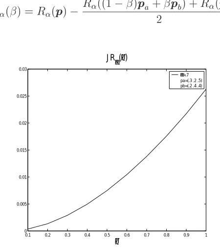
Figure 3.3: Jensen-R´enyi divergence as a function of
Proposition 3.4 Ifp a
6= p
b then the Jensen-R´enyi divergence
JR
()achieves its maximum
value when =1.
Proof: see Appendix.
Figure (3.3) illustrates the Jensen-R´enyi divergence as a function ofwhenp a
=(0:3;0:2;0:5), p
b
=(0:2;0:4;0:4)and=0:7.
3.4
The Jensen–R´enyi Divergence: Performance Bounds
In this section, performance bounds of the Jensen-R´enyi divergence in terms of the Bayes error and also of the asymptotic error of the NN classifier are derived.
Let X = fx 1
;x 2
;:::x k
gbe a set of feature vectors and C = fc 1
;c 2
;:::;c n
g be a set ofn
3.4. THE JENSEN–R ´ENYI DIVERGENCE: PERFORMANCE BOUNDS 31
vector (pattern) x 2 X to the class c = f(x). Denote X;C be two random variables
taking values inX andCrespectively. It is well known that the classifier that minimizes
the error probabilityP(f(X) 6=C)is the result of the Bayes classifier with an errorL B
written in discrete form as
L B
= inf f:X!C
Pff(X)6=Cg=1 k X j=1 max 1in f! i p ij g; where ! i
= P(C = c i
) are the class probabilities, and p ij
= P(X = x j
jC = c i
) are
the class-conditional probabilities. Denote by ! = f! i
g
1in, and p i = (p ij ) 1jk, 8i = 1;:::;n.
Proposition 3.5 The Jensen-R´enyi divergence is upper bounded by
JR ! (p 1 ;p 2
;:::;p n
)R (!) 2L B ; (3.10) whereR
(!)=R
(C), and2(0;1).
Proof: According to proposition 1, we have
R
(C) JR ! (p 1 ;p 2
;:::;p n
)=R
(CjX):
It has been proven in [63] thatH(CjX)2L
B, then (3.5) implies R
(CjX)2L
B. This
completes the proof.
A method that provides an estimate for the Bayes error without requiring knowledge of the underlying class distributions is based on the NN classifier which assigns a test pattern to the class of its closest pattern according to some metric [64].
Fornsufficiently large, the following result relating the Bayes errorL
B and the
asymp-totic errorL
NN of the NN classifier holds [64] n 1 n 1 r 1 n n 1 L NN L B L NN : (3.11)
Using (3.10), the following inequality is deduced
3.5
Image Registration with the Jensen-R´enyi Divergence
(1) (2) 50 100 150200 250 50 100 150 200 250 0 0.5 1 (3) 50 100 150200 250 50 100 150 200 250 0 0.5 1 (4)Figure 3.4: Conditional probability distributions
Letf 1
;f
2be two digital images defined on a bounded domain
N 2
, the goal of image registration is to determine the spatial transformation parameters(l
;
;
)such that (l ; ;
) = argmax (l ;;) D JR ! (f 1 ;T (l ;;) f 2 ) (3.12)
= argmax (l ;;) JR ! (p 1 (f 1 ;T (l ;;) f 2 );p 2 (f 1 ;T (l ;;) f 2
);:::;p n (f 1 ;T (l ;;) f 2 )) whereJR !
()is the Jensen-R´enyi divergence of orderand weight!.
DenoteX =fx 1
;x 2
;:::;x n
gandY =fy 1
;y 2
;:::;y n
gthe sets of pixel intensity values of f
1 and T
(l ;;) f
2 respectively, and let
3.5. IMAGE REGISTRATION WITH THE JENSEN-R ´ENYI DIVERGENCE 33
andY. p i
(f 1
;T (l ;;)
f 2
)=(p ij
)
1jnis defined as p
ij
=P(Y =y j
jX =x i
); j =1;2;:::;n
which is the conditional probability of T (l ;;)
f
2 given f
1 for the corresponding pixel
pairs. Here the Jensen-R´enyi divergence acts as a similarity measure between images. If the two images are exactly matched, thenp
i =(Æ
ij )
1jn
; i= 1;2;:::;n. Sincep 0 i
sare
degenerate distributions, by Proposition 3.2, the Jensen-R´enyi divergence is maximized for a fixed and !. Figure (3.4.1-3.4.2) show two brain MRT images in which the
misalignment is a Euclidean rotation. The conditional probability distributions fp i
g
are crisp, as in Figure (3.4.3), when the two images are aligned, and dispersed, as in Figure (3.4.4), when they are not matched.
It is worth noting that the maximization of the Jensen-R´enyi divergence holds for any
and!such that0 1and! i
0; P
i !
i
=1. If we take=1and! i
=P(X =x i
)
then, by Proposition 3.1, the Jensen-R´enyi divergence is exactly the Shannon mutual information. Indeed, the Jensen-R´enyi divergence induced similarity measure provides a more general framework for the image registration problem.
0 2 4 6 8 10 12 14 16 18 20
1 2 3 4 5 6 7 8
θ
d(A,B)
Mutual Information JR Divergence
Figure 3.5: Mutual information vs. Jensen-R´enyi divergence of uniform weights
If the two images f 1 and
T (l ;;)
f
2 are matched, the Jensen-R´enyi divergence is
maxi-mized for any valid weight. Assigning ! i
= P(X = x i
Figure (3.5) shows the registration results of the two brain images in Figure (3.4) us-ing the mutual information and the Jensen-R´enyi divergence of = 1 and uniform
weights. The peak at the matching point generated by the Jensen-R´enyi divergence is clearly much higher than the peak by the mutual information. !
i
= P(X = x i
)gives
the background pixel the largest weight. In the presence of noise, the matching in back-ground is corrupted. Mutual information may fail to identify the registration point. This phenomenon is demonstrated in Figure (3.6). The following proposition estab-lishes the optimality of the uniform weights for image registration in the context of the Jensen-R´enyi divergence.
Proposition 3.6 Letbe a uniform weight defined as i
=1=n; i =1;2;:::;nand!be any
vector such that!
i 0; P n i=1 ! i
= 1:If the misalignment between f
1 and f
2 can be modeled
by a spatial transformationT
, then the following inequality holds
JR (p 1 (f 1 ;T f 2
);:::;p n (f 1 ;T f 2
))JR ! (p 1 (f 1 ;T f 2
);:::;p n (f 1 ;T f 2
)); 82[0;1]:
(3.13)
Proof:p
i =
i,
i = 1;2;:::;n when f 1 and
f
2 are aligned by the spatial transformation T
, thenJR ! ()becomes JR ! (p 1 (f 1 ;T f 2
);:::;p n (f 1 ;T f 2
))=R ( n X i=1 ! i i )=R
(!):
Since![62] andR
()is Schur-concave, we obtainR
()R
(!). This completes
the proof of the proposition.
After assigning uniform weights to the various distributions in the Jensen-R´enyi di-vergence, a free parameter, which is directly related to the measurement sensitivity,
remains to be selected. In the image registration problem, one desires a sharp and distinguishable peak at the matching point. The sharpness of the Jensen-R´enyi diver-gence can be characterized by the maximal value as well as the width of the peak. The sharpest peak is clearly a Dirac function. The following proposition establishes that the maximal value of the Jensen-R´enyi divergence is independent of if the two images
3.5. IMAGE REGISTRATION WITH THE JENSEN-R ´ENYI DIVERGENCE 35
(1)Image A (2)Image B (3)d(A;B)
0 2 4 6 8 10 12 14 16 18 20 0.8
1 1.2 1.4 1.6 1.8 2
θ
Mutual Information JR Divergence
Figure 3.6: Registration result in the presence of the noise with =1.
Proposition 3.7 Letbe a uniform weight vector. If the misalignment betweenf 1and
f 2can
be modeled by a spatial transformationT
, then
JR
(p 1
(f 1
;T
f 2
);:::;p n
(f 1
;T
f 2
))=logn; 82[0;1]: (3.14)
In case of=0,
JR
(p 1
;p 2
;:::;p n
)=0
for any probability distributionp
isuch that
p ij
>0; i;j =1;2;:::;nand
JR
(p 1
;p 2
;:::;p n
)=logn
if and only ifp
i =
i
; i=1;2;:::;n.
Proof: see Appendix
If there exists local variation betweenf 1and
f
2, or, if the registration of the two images is
in the presence of noise, then an exact alignmentT
may not be found. The conditional probability distributionp
i (f
1 ;T
f
2
)is no longer a degenerate distribution in this case.
The following proposition establishes that taking = 1would provide a higher peak
Proposition 3.8 Letp i = i +Æp i
; i= 1;2;:::;n, whereÆp
i =(Æp
ij )
1jnis a real
distor-tion vector such thatp
ij 0; P n j=1 Æp ij
=0and P
n i=1
Æp ij
=0. Let!be a weight vector and
denoteJR
!
()as the Jensen-R´enyi divergence with=1, then we have
JR ! (p 1 ;p 2
;:::;p n
)JR ! (p 1 ;p 2
;:::;p n
); 82(0;1): (3.15)
Proof: Observe that for any probability distributionp,R
(p)H(p); 82(0;1), then, n X i=1 ! i H(p i ) n X i=1 ! i R (p i
); 82(0;1) (3.16)
SinceP n j=1 Æp ij =0; P n i=1 Æp ij
=0, and the R´enyi entropy of=1is exactly the
Shan-non entropy, the inequality (3.15) is equivalent to the inequality (3.16). This completes the proof of Proposition 3.8.
3.5.1 Discussion
0 5 10 15 20
0 1 2 3 4 5 6 7 8 θ d(A,B) (1) α=0.1 α=0.3 α=0.8 α=1.0
0 5 10 15 20
0 1 2 3 4 5 6 7 8 θ d(A,B) (2) α=0.0
Figure 3.7: Effect of the orderin image registration
In real world applications, there is a trade off between optimality and practicality in choosing . If one can model the misalignment betweenf
1 and f
2 completely and
ac-curately,=0would correspond to the best choice since it generates the sharpest peak
3.6. NUMERICAL EXPERIMENTS: ISAR IMAGE REGISTRATION 37
all thep 0 i
sthe same as the uniform distribution, ifp
i is not degenerate distribution and p
ij
>0, then the Jensen-R´enyi divergence would be zero for the whole transformation
parameter space as in case where the adapted transformation group can not “accu-rately”1model the relationship between
f 1and
f
2 accurate enough. On the other hand, = 1 is the most robust choice, in spite of also resulting in the least sharp peak. The
choice oftherefore depends largely on the accuracy of the invoked model and on the
specific application as well as the available computational resource. As an example, Figure (3.7.1) demonstrates the registration results of the two brain images in Figure (3.4) with the choice of different. In this case,=0is the best choice and would
gen-erate a Dirac function with a peak at the matching point, as illustrated in Figure (3.7.2).
3.6
Numerical Experiments: ISAR Image Registration
x y
u v
(x,y)
R(t) r(t)
θ
Figure 3.8: ISAR geometry of a moving target
Generating an ISAR image by using stepped frequency waveform [6] can be under-stood as a process of estimating the target’s two-dimensional reflectivity density func-tion (x;y) from data collected in the frequency space. Suppose a stepped frequency
burst consists of M pulses in which the transmitted frequency linearly increases from !
0 to !
0
+(M 1)!, where!
0 is the base frequency in rads/s and
!is the step
fre-quency. Let themth transmitted pulses m
(t)be a pulse of durationT
p and expressed in
complex form as
s m
(t)=e j!
m t
W(
t mT p T
p
); m =0;1;:::M 1: (3.17)
where! m
=! 0
+m!, and
W(t)= 8 < :
1; 0t<1
0; otherwise:
(3.18)
Ψ
ω ω
x y
ω0
ω0
ωM-1
ωM-1
0
Figure 3.9: Polar formatted data in spatial frequency space
Let’s define!(t) = ! 0
+(m 1)!; mT p
t < (m+1)T p
; m = 0;1;:::M 1. Under
uniform illumination, the reflected signal from the target differential areadxdyat the
target coordinate(x;y)is
h(x;y;t)=A(x;y)e
j!(t)(t 2r(t)=c)
dxdy; 0t <(M 1)T
p (3.19)
where A is a constant attenuation factor, which we can set to1 without a loss of
gen-erality. The distance between the radar antenna and the target reflection point lo-cated at (x;y) is denoted by r(t). We obtain the expression of the received signal for 0t<(M 1)T
p by integrating reflections from all the point scatterers in the target ~
g(t) = Z
+1
1 Z
+1
1
h(x;y;t)dxdy
= Z
+1 Z
+1
(x;y)e
j!(t)(t 2r(t)=c)
3.6. NUMERICAL EXPERIMENTS: ISAR IMAGE REGISTRATION 39
After quadrature demodulation, we obtain
g(t)= Z
+1
1 Z
+1
1
(x;y)e
j2!(t)r(t)=c
dxdy:; 0t <(M 1)T
p (3.21)
It can be observed from Figure (3.8) that, for target dimension that are relatively smaller than the target range R, the distance r() from the radar antenna to target reflection
point located at(x;y)is
r(t)R (t)+xcos(t) ysin(t): (3.22)
Inserting Equation (3.22) into Equation (3.21), we deduce the baseband signal in terms of target coordinate(x;y)and rotation angle
g(t)=e
j2!(t)R(t)=c Z
+1
1 Z
+1
1
(x;y)e j(x!
x (t) y!
y (t))
dxdy; 0t<(M 1)T
p (3.23)
where
! x
(t)= 2!(t)
c
cos(t) (3.24)
and
! y
(t)= 2!(t)
c
sin(t) (3.25)
are spatial frequency quantities defined at frequency!(t)and target rotation angle(t).
The phase term e
j2!(t)R(t)=c
is related to the target translational motion only, and can by compensated by traditional translational motion compensation methods.
By samplinge
j2!(t)R(t)=c
g(t)att m
=(m+ 1 2
)T p
; m = 0;1;:::(M 1), we obtain the data
collected in the frequency spaceG(m)as
G(m)= Z
+1
1 Z
+1
1
(x;y)e j(x!
x (t
m ) y!
y (t
m ))
dxdy; m=0;1;:::(M 1) (3.26)
To form a radar image,N bursts of received signal are sampled and organized burst by
burst into aMN two-dimensional array, which is shown in Figure (3.9). This sample
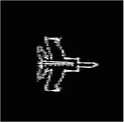
Figure 3.10: ISAR image of moving target reconstructed by the Discrete Fourier Trans-formation
ISAR image of an aircraft MIG-25 [65]. The radar is assumed to be operating at9GHz
and transmits a stepped-frequency waveform. Each burst consists of64narrow-band
pulses stepped in frequency from pulse to pulse by a fixed frequency step of 8MHz.
The pulse repetition frequency is 15KHz. Basic motion compensation processing has
been applied to the data. A total of512bursts of received signal are taken to reconstruct
the image of this aircraft, which corresponds to 2:18sintegration time. As we can see,
the resulting image is defocused due to the target rotation. In fact, the defocused im-age in Figure (3.10) is formed by overlapping a series of MIG-25s at different viewing angles. By replacing the Fourier transform with the time varying spectral analysis tech-niques [35] [65], we can take a sequence of snapshots of the target during the 2:18sof
integration time. Figure (3.11.1-3.11.6) shows the trajectory of the MIG-25, with6image
frames taken att =0:1280s; 0:4693s; 0:8107s; 1:1520s;1:4933s; 1:8347srespectively.
Image registration can be applied to estimate the target motion from this sequence of images. For the synthetic ISAR images shown in Figure(3.11), we search for the rotation anglesf
i g
N
between a sequence of image framesfI i
g N