A New Bayesian Method to Identify the Environmental Factors That Influence Recent Migration

DOI: 10.1534/genetics.107.082560

A New Bayesian Method to Identify the Environmental Factors

That Influence Recent Migration

Pierre Faubet and Oscar E. Gaggiotti

1

Ge´nomique des Populations et Biodiversite´ Laboratoire d’Ecologie Alpine, CNRS UMR 5553, Universite´ Joseph Fourier, 38041 Grenoble, France

Manuscript received September 29, 2007 Accepted for publication December 20, 2007

ABSTRACT

We present a new multilocus genotype method that makes inferences about recent immigration rates and identifies the environmental factors that are more likely to explain observed gene flow patterns. It also estimates population-specific inbreeding coefficients, allele frequencies, and local population FST’s and performs individual assignments. We generate synthetic data sets to determine the region of the parameter space where our method is and is not able to provide accurate estimates. Our simulation study indicates that reliable results can be obtained when the global level of genetic differentiation (FST) is.1%, the number of loci is only 10, and sample sizes are of the order of 50 individuals per population. We illustrate our method by applying it to Pakistani human data, considering altitude and geographic distance as explanatory factors. Our results suggest that altitude explains better the genetic data than geographic distance. Additionally, they show that southern low-altitude populations have higher migration rates than northern high-altitude ones.

T

HE study of dispersal processes is an essential problem in ecology, population genetics, conser-vation, and management of wildlife. For this reason, the estimation of migration rates has been one of the most investigated problems in population biology. Migration parameters can be directly estimated using ecological approaches such as mark-release-recapture methods but they are not applicable to the study of large or extended metapopulations. In these cases, population genetics approaches provide a better alternative because the in-formation contained in DNA can provide gene flow parameter estimates for different and complementary timescales. Methods based on coalescent theory provide long-term migration rates because they use the genea-logical information contained in a sample of genes (e.g., MIGRATE, Beerli and Felsenstein 2001). On the other hand, methods based on multilocus genotypes (e.g., BAYESASS, Wilson and Rannala 2003) provide estimates of recent immigration rates by extracting the gametic disequilibrium signal generated by immigrant individuals or their descendants.

Besides simply estimating migration rates, it is very important to identify the biotic and/or abiotic factors that influence them. This can be done by first obtaining gene flow estimates and then searching for correlations between them and various environmental variables (e.g., Giordanoet al.2007). Such an approach requires the use of summary statistics that do not take advantage of all the information contained in genetic data. An

alterna-tive approach is to implement the joint analysis of genetic and nongenetic data. Several current methods that combine both genetic and geographic data can be used to detect recent migrants (e.g., GENELAND, Guillotet al.2005; TESS, Francxoiset al.2006) but they do not take into account other environmental factors.

In previous studies we presented methods that use genetic and environmental data to study colonization processes (Gaggiottiet al.2002, 2004) and population genetic structure (Foll and Gaggiotti 2006). These approaches based on hierarchical Bayesian methods (e.g., Gelmanet al.1995) estimate the probability that a given environmental factor influences the parameters of interest (e.g., composition of colonizing groups or local population FST’s) because they explicitly model the relationship between them and the relevant ecological factors. In this article we present a new multilocus genotype method for inferring recent immigration rates and identifying the environmental factors that best ex-plain observed gene flow patterns. We use a hierarchical Bayesian approach that introduces nongenetic data through the prior distribution of the migration rates. Following Wilsonand Rannala’s (2003) approach we implement the estimation of inbreeding coefficients to allow for departures from Hardy–Weinberg equilibrium within local populations. Finally, the method infers the population ancestry of individuals by assigning their alleles to populations from which they originated. We carry out a simulation study to identify the region of parameter space where the method is and is not able to provide accurate posterior estimates. We also illustrate our method with a real data example.

1_{Corresponding author: LECA, BP 53, 2233 Rue de la Piscine, 38041}

Grenoble Cedex 9, France. E-mail: [email protected]

DATA AND MODEL PARAMETERS

Inferring migration rates from genetic data: The method is based on a population genetics model that differs from that used by Wilsonand Rannala(2003). More specifically, instead of assuming that sampling takes place right after migration, we consider that this is done after reproduction and before migration. Let us consider a metapopulation of a diploid species with nonoverlapping generations that is subdivided into I demes that can exchange migrants. Let X¼ ðXhlÞ be

the observed multilocus genotypes of n individuals scored atLmarker loci, whereXhldenotes the genotype

of individualhat locusl. We assume thatniindividuals

were sampled from population i and use the vector S¼ ðShÞ to identify the population Sh where the

in-dividualhwas sampled from.

Population allele frequencies are given by a matrixp composed of vectorsp_il¼ ðpilaÞthat give the frequency

of alleleaat locuslfor populationi. Following Falush

et al.(2003), we consider a model with correlated allele

frequencies based on the approach introduced by Balding and Nichols (1995). Thus, we assume that before the last generation, the population was at migration–drift equilibrium so that allele frequencies in each population are determined by the global allele frequencies in the metapopulation as a whole,p˜_l ¼ ð˜plaÞ,

and the degree of genetic differentiation between each local population and the overall metapopulation,u¼ ðu_iÞ, whereui¼1=FSTi 1. Finally, to allow departures from Hardy–Weinberg equilibrium, we introduce population-specific inbreeding coefficientsF¼ ðFiÞ, whereFiis the

inbreeding coefficient for populationi. Thus, we con-sider two levels of inbreeding, one at the population level corresponding toFSTand another one at the in-dividual level, corresponding toFIS.

Instead of focusing directly on individual migration rates, we consider the probability that genes in a deme originated in another one over the last generation. Thus, migration is described by a matrix m¼ ðmijÞ,

wheremijis the probability that alleles in populationi

came from populationjduring the previous generation. The ancestral state of the individuals is described by a matrix M¼ ðMhÞ, where Mh¼ ði;jÞ is a two-element

vector identifying the source demes (iandj) for the two alleles of individual h. All possible ancestry states are considered: both alleles come from the deme where the individual was sampled, or both come from another deme, or they come from two different ones. Thus, migration rates for individuals are obtained as

˜ mijk¼

m2_ij ifj¼k

2mijmik ifj6¼k

; j#k; (

ð1Þ

where m˜ijk is the probability that individuals sampled

from populationi belong to the ancestry class (j, k). Note that our approach estimates migration rates only over the last generation. Moreover, as opposed to Wilson

and Rannala(2003) migration rates vary freely in the interval (0, 1) and do not have to be small.

The model parameters described above (p;p˜;u;F;

M;m) are estimated from the genetic data using a Bayesian approach and Markov chain Monte Carlo (MCMC) techniques.

Likelihood:The likelihood is the probability of the

ob-served genotypes given model parameters and is con-structed by defining the probability of observing the genotype of individual h at locus l in terms of the ancestry classes. We note these genotypes Xhl¼ ðXhl1; Xhl2Þ, whereXhlcis the allele observed at locuslin

chro-mosomec¼1, 2 of individualh. Thus, individualh ge-notype likelihood at locuslis given by

PrðXhljMh;F;pÞ ¼

fðXhl;iÞ ifMh¼ ði;iÞ pilXhl1pjlXhl21gpjlXhl1pilXhl2 ifMh¼ ði; jÞ;

(2)

where

fðXhl; iÞ ¼

ð1FiÞpilX2 hl11FipilXhl2 ifXhl1 ¼Xhl2

2ð1FiÞpilXhl1pilXhl2 otherwise (

ð3Þ

and

g¼ 0 ifXhl1¼Xhl2

1 otherwise:

ð4Þ

The first case considered in Equation 2 corresponds to the scenario where both alleles originated in the same source population, in which case we need to take into account possible deviations from Hardy–Weinberg equi-librium (see Equation 3). The second case considers that the individual is the descendant of parents that come from two different source populations, in which case we need to take into account that there are two different ways of assigning the alleles to the parents.

If we assume that individuals were sampled at random and loci are unlinked, then the likelihood of the whole sample is obtained by multiplying across all loci and individuals,

PrðXjM;F;pÞ ¼Y

n

h¼1 YL

l¼1

PrðXhljMh;F;pÞ: ð5Þ

This likelihood can be used as the basis for inference using a Bayesian approach.

Combining genetic and environmental data:One can expect that migration patterns are influenced by envi-ronmental factors such as population densities, distan-ces between local populations, etc. To identify which environmental factors have influenced gene flow we use Gaggiottiet al.’s (2004) approach. Let us suppose that our knowledge of the species under study leads us to think that R environmental factors G¼ ðGðrÞ_{Þ may}

mi-gration rates. More specifically, we focus on the ancestry of immigrant alleles by conditioning on not being a resident allele

mw_ij ¼ mij

1mii

ð6Þ

and assume that the vector mw

i ¼ ðm

w

ijÞj6¼i follows a

Dirichlet distribution;i.e.,mw

i jciDirðciÞ, whereci¼

ðc_ijÞ_j6¼i are shape parameters for the Dirichlet

distribu-tion. Furthermore, we assume that each shape parameter

cijfollows a lognormal distribution;i.e., for each pair of

distinct populationsi6¼j

logc_ij N ðm_ij;s2_{Þ; ð7Þ}

where the meanmij is given by the generalized linear

regression

m_ij¼a01 X

r

arG ðrÞ

ij 1

X

r,s

arsG ðrÞ

ij G

ðsÞ

ij ; ð8Þ

where ardenotes the effect of environmental factor r

and ars denotes the effect of first-order interactions

between factorsrands; these parameters are collected into a single vectora¼ ðar;arsÞ. The sign and the

mag-nitude of the a’s tell us about the direction and the strength of the environmental factors. Finally, s2 _is

the amount of variation that remains unexplained by the regression andGijðrÞis the observed value for factorr,

which is hypothesized to influence migration between populations i and j. To reduce posterior correlation and to simplify prior elicitation and posterior interpre-tation process, explanatory factors are normalized before analysis so that they have zero mean and variance one.

By excluding different regression terms we can define different alternative models. We note, however, that as opposed to previous applications of this approach (cf. Gaggiottiet al.2004; Folland Gaggiotti2006), the intercept a0is included in all models because it takes into account the effect of factors that act at a geographic scale larger than that of the metapopulation under study (seediscussionfor more details).

Other priors: We assume that there is no prior

infor-mation on the shape of the other parameters and, therefore, adopt the vague priors that are given in the appendix. Note that in the particular case of the

prob-ability to observe nonmigrant genes (i.e.,mqq), we adopt

a uniform prior between 0 and 1 because, although some environmental factors may influence whether or not an individual decides to emigrate, our method is aimed at estimating immigration rates and, therefore, cannot take into account this possibility.

Posterior distribution:The model is now expressed in terms of parametersQ¼ ðp;p˜;u;F;M;m;c;a;s2_Þand the corresponding posterior distribution is given by Bayes’ rule:

ð9Þ

The full model is represented by the directed acyclic graph (DAG) in Figure 1.

The posterior distributions of parameters given in Equation 9 are estimated using MCMC methods that are described in the supplemental information.

Posterior model probabilities: Besides estimating migration rates our method is aimed at identifying the environmental factors influencing gene flow. As we mentioned before, several alternative models can be obtained from the full regression (8) by canceling ele-ments of the vectora. Note that models that include first-order interactions between factors rands are allowed only if both factors are included. Thus for modelM, the corresponding posterior distribution is given by

Figure1.—The DAG for the model given in Equation 9.

fðQMjX;S;GÞ

}PrðXjM;F;pÞPrðMjS;mÞfðFÞfðpjp˜;uÞfðp˜ÞfðuÞ

3fðmjcÞfðcjaM;s2;GÞfðaMÞfðs2ÞPrðMÞ; ð10Þ

whereQMis the parameter vector under modelM,aM

is the corresponding regression vector, and PrðMÞ

denotes prior model probability. Posterior model prob-abilities are estimated using the reversible-jump (RJ) MCMC approach (Green1995, detailed in supplemen-tal information). Here we note only that one of the problems faced when estimating posterior model prob-abilities is that the prior fors2

acan have a large effect on the estimates. When very vague priors are used, more posterior weight is placed on the model with the fewest parameters. This is the well-known Jeffreys–Lindley paradox (Robert1994). This problem was avoided by first running an MCMC of the full model with vague priors and then using the posterior estimates of thea’s as informative priors for a new MCMC run.

SIMULATION STUDY

We evaluated the sensitivity of our method by gener-ating synthetic data under a particular scenario in which gene flow is influenced by two factors. We considered various levels of genetic differentiation and migration rates. We are interested in the ability of our algorithm to find the correct scenario and to provide accurate pos-terior estimates for migration rates (with corresponding fairly narrow highest posterior density intervals, HPDI).

Generation of synthetic data: We simulated data following the inference model presented in Figure 1. We initially considered a scenario withI¼4 populations, each with local population sizes ofNi¼5000 individuals.

The sample size per population was ni ¼100 and we

assumed that each sampled individual was scored for L¼10 polymorphic loci, each withK¼10 alleles.

Generating migration rates from environmental factors: We consider two environmental factors that could be, for example, geographic distance (G1) and population density (G2). The pairwise geographic distances were generated using a standard normal distribution. The pairwise differences in population density were generated by first filling the top triangular matrix with values drawn from a standard normal and then filling the bottom triangular matrix with the opposite values. This procedure is equivalent to standardizing the observed pairwise differences in environmental factors before analysis.

To generate the migration matrix, we first chose the values for the diagonal elements (proportion of non-migrant genes) and then we calculated the values for the nondiagonal elements (immigration rates) using the following procedure. We seta1¼ 0.9, a2¼1.1, and

a₁₂¼0 (i.e., no interaction effect) and calculatedm_ij’s using Equation 8. Assuming no deviation from the linear

regression (i.e., s2 _{¼ 0), we set c} ij¼e

m_ij

. Finally we computed the means E½mijwjci ¼cij=

P

j6¼icij of the

Dirichlet distribution used for the migration rates (Equation A2) and rescaled them so that they added up to 1mii.

Genetic data:To generate multilocus genotypes with a

given level of genetic differentiation, we need to generate parametric allele frequencies. This task was performed using Baldingand Nichols’(1997) sampling formula forFST. According to this formula, genes are sampled one by one during an iterative process. The probability that the next gene sampled isaafter having sampledngenes of whichnacorrespond to alleleais given by

paðna;nÞ ¼

naFST1ð1FSTÞpa 11ðn1ÞFST

; ð11Þ

where pa is the global frequency of allele a in the

metapopulation.

To generate the parametric allele-frequency distribu-tion of each locus in any given local populadistribu-tion for a givenFSTvalue, we first sample an allele at random from the metapopulation allele-frequency distribution and then use Equation 11 to calculate the probability distri-bution for the type of the allele that will be sampled next. Using this distribution we obtain the next allele. This process is repeated iteratively until we obtain the 2Ni alleles present in local populationi. We used

uni-form allele frequencies for the metapopulation. Large departures from the target FST value were avoided by using the following iterative process. We generated the local population’s allele-frequency distri-butions and calculated the global and pairwiseFST’s. If one or more of these values were not within 10% of the target value we discarded the allele frequencies and generated new ones. If the new allele frequencies sat-isfied the requirement, we generated the genotypes; otherwise we continued this iterative procedure until the constraint was satisfied. This procedure was used to control for the effect of genetic differentiation on the performance of the method.

Using the gene migration rates calculated above, we obtained the proportion of migrant individuals in each population using Equation 1. Multilocus genotypes for each local population were generated assuming Hardy– Weinberg equilibrium. Genotypes of nonmigrant indi-viduals were obtained by drawing two alleles from the local population allele-frequency distribution. For the migrant individuals with both parents coming from the same local population, the genotype was obtained by drawing two alleles at random from the parents’ source population. For migrant individuals with parents com-ing from different source populations, we sampled one allele from the source population of each parent. Finally, samples were generated by drawingni

Implementation details: Each MCMC was run for 1,030,000 iterations. The first 20,000 iterations consist of short pilot runs used to tune up the proposal distri-butions to obtain acceptance rates between 25 and 45%. The next 10,000 iterations were discarded as burn-in and the remaining observations were sampled every 100 itera-tions, giving a sample size of 10,000 for each analysis.

To take into account model uncertainty, parameters are estimated using Bayesian model-averaging methods. The only exception to this rule are the regression pa-rameters, which are model specific and, therefore, were estimated using the subset of values corresponding to the model with the highest posterior probability. Finally, posterior model probabilities are obtained by observing the number of times the chain visits each alternative model. Posterior estimates are based on the sample mean except for the deviation from the regressions2_{, which}

usually has a highly asymmetric posterior distribution. In this latter case we used the posterior mode, which was estimated using kernel density estimation.

We investigated the effect of varying three parame-ters: the level of genetic differentiation, FST ¼ {0.01, 0.05, 0.10, 0.25}; the proportion of nonmigrant alleles, mii¼{0.7, 0.9}; and the number of populations,I¼{4, 6}.

For each parameter set we generated 10 independent genetic data sets as described above. The results we present below are averages across these 10 replicates. As a measure of accuracy we also present the relative mean square errors (RMSE).

Results: We investigated the performance of our method to provide reliable estimates under different scenarios of migration and genetic differentiation and number of populations studied. We consider first the effects on model determination, and then we address the influence on migration rate estimates and finally on individual assignments.

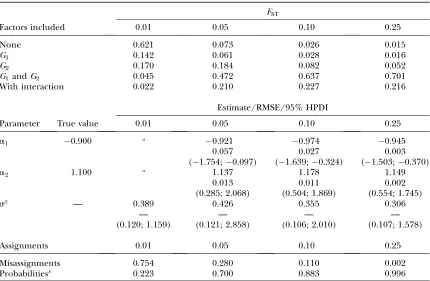
When the immigration rate is high (mii ¼ 0.7; see

Table 1), estimates of posterior model probabilities are strongly influenced by the degree of genetic differenti-ation (FST). When differentiation is low (FST¼0.01), the method fails to identify the model used to generate the synthetic data. However, the correct model is identified when FST . 0.01, and, moreover, its posterior model probability increases steadily with increasing genetic differentiation. The estimation of regression parame-ters is also influenced by the magnitude ofFSTbut to a lesser degree. The RMSE decreases with increasing genetic differentiation but the bias is largely unaffected.

TABLE 1

Posterior estimates for various levels of genetic differentiation and high gene flow

FST

Factors included 0.01 0.05 0.10 0.25

None 0.621 0.073 0.026 0.015

G1 0.142 0.061 0.028 0.016

G2 0.170 0.184 0.082 0.052

G1andG2 0.045 0.472 0.637 0.701

With interaction 0.022 0.210 0.227 0.216

Estimate/RMSE/95% HPDI

Parameter True value 0.01 0.05 0.10 0.25

a1 0.900 a 0.921 0.974 0.945

0.057 0.027 0.003

(1.754;0.097) (1.639;0.324) (1.503;0.370)

a₂ 1.100 a _{1.137 1.178 1.149}

0.013 0.011 0.002

(0.285; 2.068) (0.504; 1.869) (0.554; 1.745)

s2 _{— 0.389 0.426 0.355 0.306}

— — — —

(0.120; 1.159) (0.121; 2.858) (0.106; 2.010) (0.107; 1.578)

Assignments 0.01 0.05 0.10 0.25

Misassignments 0.754 0.280 0.110 0.002

Probabilitiesb _{0.223 0.700 0.883 0.996}

Posterior model probabilities, regression parameter mean estimates, and assignment accuracy for synthetic data generated with proportions of nonmigrant alleles set tomii¼0.70 are shown.

Thus, it is the accuracy of the estimates (as illustrated by the HPDIs) that is influenced byFST. The proportion of the variance that remains unexplained by the model,s2_,

decreases as genetic differentiation increases.

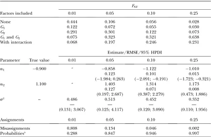
Decreasing the immigration rate (mii ¼0.90) has a

detrimental effect on estimates (Table 2). Although the true model is correctly identified for FST . 0.01, its posterior probability is lower than that observed when mii¼0.70. Estimates of regression parameters are more

biased and less accurate (wider HPDIs), leading to higher RMSEs. Also, the proportion of the variance that remains unexplained,s2_{, is larger. Note, however, that}

as was the case before, the quality of all estimates im-proves with increasing genetic differentiation.

Increasing the number of populations studied (I¼6) improves model determination (Table 3). More precisely, the posterior probability of the true model is strongly increased and the proportion of variance that remains unexplained decreases sharply (see Table 3 and last columns of Tables 1 and 2). However, the effect on the quality of the regression parameter estimates is some-what decreased since the bias and the RMSE increase. Nevertheless, the width of the HPDIs decreases, in-dicating that the precision increases.

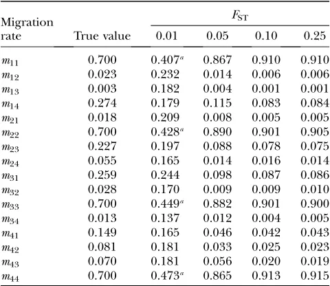
Estimates of gene migration rates improve with in-creasing genetic differentiation (Table 4). The bias de-creases sharply betweenFST ¼0.01 and 0.1 and then remains very low. Note that the only cases where the HPDI does not include the true value correspond to the case with the weakest genetic differentiation (FST¼0.01). When the number of nonmigrant genes decreases we observe the same pattern but in this case the number of estimates for which the HPDIs do not include the true value is smaller and corresponds only to the estimates of nonmigrant proportions (Table 5).

In terms of posterior individual assignments, increas-ing genetic differentiation improves the quality of the estimation (see the bottom three rows of Tables 1 and 2). That is, the proportion of individuals that are misas-signed decreases while the average posterior assignment probability increases. Decreasing the proportion of mi-grant genes also improves the quality of assignments; the proportion of misassignments decreases and the average posterior probabilities with which individuals are as-signed increase. The effect of varying the number of populations is very small, being somewhat more distin-guishable when the proportion of nonmigrants is larger (see bottom three rows of Tables 1–3).

TABLE 2

Posterior estimates for various levels of genetic differentiation and low gene flow

FST

Factors included 0.01 0.05 0.10 0.25

None 0.444 0.106 0.056 0.028

G1 0.122 0.072 0.055 0.030

G2 0.291 0.301 0.122 0.073

G1 andG2 0.075 0.323 0.521 0.638

With interaction 0.068 0.197 0.246 0.231

Estimate/RMSE/95% HPDI

Parameter True value 0.01 0.05 0.10 0.25

a1 0.900 a 0.858 1.122 1.010

0.123 0.101 0.015

(1.984; 0.263) (2.091;0.191) (1.723;0.321)

a₂ 1.100 a _{1.403 1.314 1.173}

0.127 0.071 0.008

(0.197; 2.687) (0.387; 2.279) (0.473; 1.886)

s2 _{– 0.486 0.513 0.452 0.352}

— — — —

(0.131; 3.067) (0.125; 4.117) (0.120; 3.090) (0.110; 1.956)

Assignments 0.01 0.05 0.10 0.25

Misassignments 0.808 0.134 0.046 0.002

Probabilitiesb _{0.288 0.847 0.946 0.997}

Posterior model probabilities, regression parameter mean estimates, and assignment accuracy for synthetic data generated with proportions of nonmigrant alleles set tomii¼0.90 are shown.

a_{The corresponding regression parameter is not included in the model with the highest posterior model}

probability.

We also investigated what is the effect of using ex-plicative variables that are different from the ones used to generate the synthetic data. The results (Table 6) show that the highest posterior probability is assigned to the null model, which indicates that the method does not wrongly identify as important factors that are not responsible for the observed migration pattern.

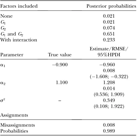
It is also important to investigate the effect of the amount of data used for the estimation, which can be characterized by the sample sizes and number of loci scored. The effect of decreasing the sample size from 100 to 50 individuals per population does not have much of an effect on posterior model probabilities while estimates of regression parameters have a slightly larger bias and wider HPDIs leading to somewhat larger RMSEs (com-pare last column of Table 1 with Table 7). Migration rate estimates show no increase in bias but their HPDIs are larger (compare Tables 8 and 9). Finally, the quality of the assignments is barely influenced by a decrease in the sample sizes (compare Tables 1 and 7). The effect of increasing the number of loci scored from 10 to 20 does not have an effect on model determination, estimates of regression parameters, and migration rates when the

level of genetic differentiation is moderate (FST ¼0.1) (results not shown). The only result that changes is the proportion of individuals that are misassigned, which decreases from 0.002 to 0. We also carried out analysis of a

TABLE 3

Posterior estimates for the scenario with six populations

FST¼0.25

Factors included mii¼0.70 mii¼0.90

None 0.000 0.000

G1 0.000 0.000

G2 0.000 0.001

G1andG2 0.915 0.883

With interaction 0.085 0.116

Estimate/RMSE/95%HPDI

Parameter True value mii¼0.70 mii¼0.90

a1 0.900 1.056 1.022

0.031 0.022

(1.416;0.707) (1.521;0.537)

a₂ 1.100 1.244 1.246

0.018 0.018

(0.960; 1.531) (0.856; 1.659)

s2 _{— 0.164 0.213}

— —

(0.080; 0.381) (0.096; 0.566)

Assignments mii¼0.70 mii¼0.90

Missassignments 0.010 0.002 Probabilitiesa _{0.985 0.997}

Model determination, regression parameters, mean esti-mates, and assignment accuracy for synthetic data when vary-ing nonmigrant gene proportionsmii.

a

Maximum posterior assignment probabilities averaged across all individuals.

TABLE 4

Migration estimates for various levels of genetic differentiation and high migration rate

Migration rate

FST

True value 0.01 0.05 0.10 0.25

m11 0.700 0.355a _{0.663 0.702 0.710}

m12 0.023 0.173 0.036 0.021 0.020 m13 0.003 0.222a _{0.007 0.002 0.002}

m14 0.274 0.250 0.293 0.275 0.269 m21 0.018 0.184 0.027 0.021 0.020 m22 0.700 0.359a _{0.656 0.720 0.710}

m23 0.227 0.252 0.240 0.213 0.220 m24 0.055 0.205 0.076 0.047 0.050 m31 0.259 0.224 0.291 0.273 0.256 m32 0.028 0.252a _{0.029 0.027 0.025}

m33 0.700 0.336a _{0.662 0.689 0.704}

m34 0.013 0.188a _{0.020 0.010 0.014}

m41 0.149 0.243 0.151 0.136 0.142 m42 0.081 0.211 0.111 0.085 0.079 m43 0.070 0.185 0.074 0.061 0.064 m44 0.700 0.362a _{0.664 0.719 0.715}

Posterior estimates averaged across analyses of 10 simulated data sets with proportions of nonmigrant alleles set tomii¼

0.70 are shown.

a

The 95% HPDI does not contain the true value.

TABLE 5

Migration estimates for various levels of genetic differentiation and high migration rate

Migration rate

FST

True value 0.01 0.05 0.10 0.25

m11 0.700 0.407a _{0.867 0.910 0.910}

m12 0.023 0.232 0.014 0.006 0.006 m13 0.003 0.182 0.004 0.001 0.001 m14 0.274 0.179 0.115 0.083 0.084 m21 0.018 0.209 0.008 0.005 0.005 m22 0.700 0.428a _{0.890 0.901 0.905}

m23 0.227 0.197 0.088 0.078 0.075 m24 0.055 0.165 0.014 0.016 0.014 m31 0.259 0.244 0.098 0.087 0.086 m32 0.028 0.170 0.009 0.009 0.010 m33 0.700 0.449a _{0.882 0.901 0.900}

m34 0.013 0.137 0.012 0.004 0.005 m41 0.149 0.165 0.046 0.042 0.043 m42 0.081 0.181 0.033 0.025 0.023 m43 0.070 0.181 0.056 0.020 0.019 m44 0.700 0.473a _{0.865 0.913 0.915}

Posterior estimates averaged across analyses of 10 simulated data sets with proportions of nonmigrant alleles set tomii¼

0.90 are shown.

a

scenario with FST ¼ 0.05 and in this case, increasing the number of loci from 10 to 20 decreased the width of the HPDIs for migration rate estimates and improved the

accuracy of individual assignments. APPLICATION TO REAL DATA

We use the human genome diversity cell line panel– Centre d’Etude du Polymorphisme Humain (HGDP– CEPH) presented by Cannet al.(2002) to illustrate how our method can be used to make inferences about the

TABLE 6

Posterior model estimates when testing for nonexplanatory factors

FST

Factors included 0.01 0.05 0.10 0.25

None 0.636 0.533 0.512 0.505

G1 0.127 0.224 0.243 0.241

G2 0.184 0.157 0.151 0.158

G1andG2 0.039 0.065 0.071 0.076 With interaction 0.013 0.022 0.022 0.021

FST

Assignments 0.01 0.05 0.10 0.25

Misassignments 0.741 0.282 0.110 0.002 Probabilities 0.218 0.694 0.881 0.996

Posterior model probabilities and assignment accuracy when varying the level of genetic differentiationFSTand test-ing for two nonexplanatory factors (i.e., different from the ones we used for generating migration rates) are shown. Data were simulated with proportions of nonmigrant alleles set to mii¼0.70.

TABLE 7

Model estimates when sampling 50 individuals per population

Factors included Posterior probabilities

None 0.021

G1 0.021

G2 0.074

G1andG2 0.651

With interaction 0.233

Parameter True value

Estimate/RMSE/ 95%HPDI

a₁ 0.900 0.960

0.008 (1.608;0.322)

a₂ 1.100 1.208

0.014 (0.536; 1.909)

s2 _{– 0.349}

(0.108; 1.922)

Assignments

Misassignments 0.008

Probabilities 0.989

Posterior model probabilities, regression parameter mean estimates, and assignment accuracy for synthetic data gener-ated with proportions of nonmigrant alleles set to mii ¼

0.70 and level of genetic differentiation set to FST ¼ 0.25 are shown.

TABLE 8

Migration estimates when sampling 50 individuals per population

Parameter

True value

Posterior

estimate RMSE 95% HPDI

m11 0.700 0.702 ,0.001 (0.612; 0.790) m12 0.023 0.026 0.043 (0.003; 0.056) m13 0.003 0.002 0.070 (0.000; 0.010) m14 0.274 0.270 0.001 (0.185; 0.356) m21 0.018 0.011 0.149 (0.000; 0.029) m22 0.700 0.722 0.001 (0.632; 0.808) m23 0.227 0.220 0.001 (0.142; 0.301) m24 0.055 0.047 0.025 (0.013; 0.086) m31 0.259 0.238 0.007 (0.158; 0.322) m32 0.028 0.026 0.030 (0.003; 0.055) m33 0.700 0.725 0.001 (0.637; 0.811) m34 0.013 0.011 0.033 (0.000; 0.028) m41 0.149 0.136 0.008 (0.074; 0.201) m42 0.081 0.075 0.006 (0.031; 0.124) m43 0.070 0.067 0.001 (0.025; 0.115) m44 0.700 0.721 0.001 (0.634; 0.808)

Estimates based on the posterior mean, RMSE, and 95% HPDI are reported for synthetic data generated with propor-tions of nonmigrant alleles set tomii¼0.70 and the level of

genetic differentiation set toFST¼0.25.

TABLE 9

Migration rate estimates when sampling 100 individuals per population

Parameter

True value

Posterior

estimate RMSE 95% HPDI

m11 0.700 0.710 ,0.001 (0.647; 0.772) m12 0.023 0.020 0.018 (0.004; 0.038) m13 0.003 0.002 0.218 (0.000; 0.006) m14 0.274 0.269 ,0.001 (0.208; 0.323) m21 0.018 0.020 0.014 (0.005; 0.038) m22 0.700 0.710 ,0.001 (0.647; 0.772) m23 0.227 0.220 0.001 (0.165; 0.277) m24 0.055 0.050 0.009 (0.023; 0.079) m31 0.259 0.256 ,0.001 (0.198; 0.317) m32 0.028 0.025 0.009 (0.007; 0.046) m33 0.700 0.704 ,0.001 (0.640; 0.766) m34 0.013 0.014 0.013 (0.002; 0.029) m41 0.149 0.142 0.002 (0.097; 0.190) m42 0.081 0.079 0.001 (0.045; 0.115) m43 0.070 0.064 0.007 (0.033; 0.098) m44 0.700 0.715 ,0.001 (0.652; 0.777)

Estimates based on the posterior mean, RMSE, and 95% HPDI are reported for synthetic data generated with propor-tions of nonmigrant alleles set tomii¼0.70 and the level of

factors influencing migration patterns. In our example we selected a subset of eight populations, all from Pakistan (see Figure 2), corresponding to 200 individ-uals (25 per population). We grouped together the Balochi and Brahui samples because the STRUCTURE analyses carried out by Rosenberget al. (2002) place them in the same genetic cluster (see their Figure 2). Also, instead of using all 377 loci we did a first screening using an improved version of Beaumontand Balding’s (2004) method to identify outlier loci that could be influenced by selection. On the basis of this screening we selected a total of 247 loci that were used in the analysis. The effect of distance is supposed to be one of the main factors in determining gene flow in many species, but other factors such as altitude can influence geo-graphic isolation and, therefore, migration patterns. We use our method to evaluate the relative importance of these two factors. We obtained pairwise geographic distances from latitude and longitude coordinates and also calculated the difference in altitude between each focal population and all other populations. Cannet al. (2002) give the geographic coordinates of each popula-tion as sample intervals; thus we used the gravity center of the area for the calculation of geographic distances be-tween populations. With two parameters we can define five alternative models, which are presented in Table 10. As was the case for the simulation study we used short pilot runs to tune up the proposal distributions to achieve reasonable acceptance ratios. To ensure convergence we increased the burn-in to 106_{and the sample size to 20,000}

and used a thinning interval of 50 iterations.

Some of the population-specificFSTvalues are,0.01 (see Table 11), the level of genetic differentiation that our simulation study identified as problematic for the

estimation of parameters. This example, therefore, provides us with an opportunity to illustrate the prob-lems that may arise when our method (or any other MCMC-based method) is used in scenarios with weak genetic differentiation. In these situations, it is neces-sary to run many independent replicates and compare their results; in the present case we used 10 runs. In 6 of

Figure2.—Geographic locations of sampled populations.

Solid circles represent centers of gravity of sampled areas of Pakistan. Abbreviations for population names are as follows: Ba, Balochi; Br, Brahui; Bu, Burusho; Ha, Hazara; Ka, Kalash; Ma, Makrani; Pa, Pathan; Si, Sindhi.

TABLE 10

Posterior model probabilities for the Pakistani human data set

Factors included

Estimate/95% HPDI

Pr(M) a₁ a₂ a₃

None 0.064

Distance 0.093 0.756 (2.88; 0.417)

Altitude 0.550 1.74

(3.35; 0.338) Distance and

altitude

0.232 0.469 1.55 (2.95; 0.639)(2.91; 0.747) With

interaction

0.061 0.524 1.64 0.302 (2.66; 0.71) (3.4; 0.599) (1.2; 1.44)

Posterior model probabilities for the human data set when considering geographic distances and differences in altitudes as environmental factors are shown. Posterior estimates for re-gression parameters are based on the mode and 95% HPDI. The maximuma posterioriestimate ofs2_{is 0.657 with the 95%} HPDI ranging from 0.089 to 11.1.

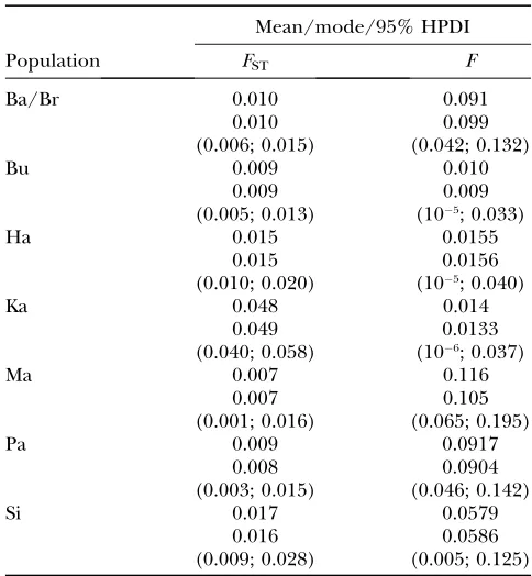
TABLE 11

Local populationFST’s and inbreeding coefficient

for Pakistani populations

Mean/mode/95% HPDI

Population FST F

Ba/Br 0.010 0.091

0.010 0.099

(0.006; 0.015) (0.042; 0.132)

Bu 0.009 0.010

0.009 0.009

(0.005; 0.013) (105_{; 0.033)}

Ha 0.015 0.0155

0.015 0.0156

(0.010; 0.020) (105_{; 0.040)}

Ka 0.048 0.014

0.049 0.0133

(0.040; 0.058) (106_{; 0.037)}

Ma 0.007 0.116

0.007 0.105

(0.001; 0.016) (0.065; 0.195)

Pa 0.009 0.0917

0.008 0.0904

(0.003; 0.015) (0.046; 0.142)

Si 0.017 0.0579

0.016 0.0586

(0.009; 0.028) (0.005; 0.125)

them, the most probable model included altitude only and in all cases there was a posterior probability of at least 50%. The second most probable model included both factors. However, in 4 other runs two other models, one including distance only and the other including both distance and altitude, gave similar high posterior probabilities while the model including altitude only was ranked third. Given these results, we followed Faubetet al.(2007) and chose the run with the lowest deviance for estimation purposes. The Bayesian devi-ance has been proposed as a measure of model fit by a number of authors (Faubetet al.2007 and references therein) and in our specific case we considered the assignment component of the total deviance,Dassign ¼ 2 log PrðMjS;mÞ. Table 10 presents these results. The model with the highest posterior probability includes altitude only and the second most probable model includes both altitude and distance. In this latter case, the regression coefficients for the effects of altitude and distance are both negative, indicating that, as expected, both factors decrease migration rates between popula-tions. Note, however, that the former seems to have a stronger effect (i.e., larger absolute value).

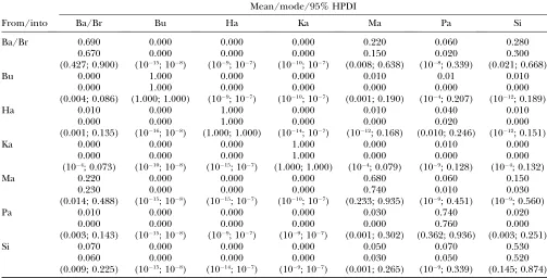
Table 12 presents the mode and HPDI of migration rates between populations. Although the sum of max-imum posterior estimates does not necessarily add up to one, we used them as estimators because of the inherent asymmetry of migration rate posterior distributions. There are three populations that do not receive mi-grants (Burusho, Bu; Hazara, Ha; and Kalash, Ka) and

they correspond to those located in high-altitude areas. Moreover, two of these populations (Bu and Ka) do not seem to send migrants either and a third one (Ha) seems to contribute very little to the gene pool of the Pathan. The population with the highest proportion of migrant genes is the Sindhi, which receives migrants mainly from Balochi/Brahui (Ba/Br). Three other pop-ulations have a somewhat lower proportion of migrant genes (Ba/Br; Makrani, Ma; and Pathan, Pa). In the case of Ba/Br, most of the genes come from Ma, and, con-versely, most of the genes of Ma come from Ba/Br. Finally, the Pathan receive similar proportions of genes from Ba/Br, Ha, and Sindhi (Si). In general, there are frequent gene exchanges among southern populations while northern populations remain fairly isolated. The best explanation for this migration pattern is altitude differences with the most isolated populations being at high altitude and the least isolated ones at low altitude. Finally, the mean and mode of inbreeding coefficient estimates are somewhat large when compared to FST estimates but this is not the case if we compare the lower bounds of the HPDIs (Table 11). Still, there are three local populations (Ba/Br, Ma, and Pa) for which the lower bound ofFISHPDIs is.0.04 while that ofFST’s is much lower. A potential explanation for this result could be that samples were taken from adult individuals and, therefore, the data set does not fit model assump-tions concerning the moment at which sampling takes place. However, we do not have information concerning the age group involved in the sampling.

TABLE 12

Migration rates between Pakistani populations

Mean/mode/95% HPDI

From/into Ba/Br Bu Ha Ka Ma Pa Si

Ba/Br 0.690 0.000 0.000 0.000 0.220 0.060 0.280

0.670 0.000 0.000 0.000 0.150 0.020 0.300

(0.427; 0.900) (1015_{; 10}8_{) (10}9_{; 10}7_{) (10}10_{; 10}7_{) (0.008; 0.638) (10}8_{; 0.339) (0.021; 0.668)}

Bu 0.000 1.000 0.000 0.000 0.010 0.01 0.010

0.000 1.000 0.000 0.000 0.000 0.000 0.000

(0.004; 0.086) (1.000; 1.000) (109_{; 10}7_{) (10}10_{; 10}7_{) (0.001; 0.190) (10}4_{; 0.207) (10}12_{; 0.189)}

Ha 0.010 0.000 1.000 0.000 0.010 0.040 0.010

0.000 0.000 1.000 0.000 0.000 0.020 0.000

(0.001; 0.135) (1016_{; 10}8_{) (1.000; 1.000) (10}14_{; 10}7_{) (10}12_{; 0.168) (0.010; 0.246) (10}12_{; 0.151)}

Ka 0.000 0.000 0.000 1.000 0.000 0.010 0.000

0.000 0.000 0.000 1.000 0.000 0.000 0.000

(104_{; 0.073) (10}10_{; 10}8_{) (10}15_{; 10}7_{) (1.000; 1.000) (10}4_{; 0.079) (10}9_{; 0.128) (10}4_{; 0.132)}

Ma 0.220 0.000 0.000 0.000 0.680 0.060 0.150

0.230 0.000 0.000 0.000 0.740 0.010 0.030

(0.014; 0.488) (1015_{; 10}8_{) (10}15_{; 10}7_{) (10}10_{; 10}7_{) (0.233; 0.935) (10}9_{; 0.451) (10}9_{; 0.560)}

Pa 0.010 0.000 0.000 0.000 0.030 0.740 0.020

0.000 0.000 0.000 0.000 0.000 0.760 0.000

(0.003; 0.143) (1015_{; 10}8_{) (10}9_{; 10}7_{) (10}9_{; 10}7_{) (0.001; 0.302) (0.362; 0.936) (0.003; 0.251)}

Si 0.070 0.000 0.000 0.000 0.050 0.070 0.530

0.060 0.000 0.000 0.000 0.030 0.050 0.520

(0.009; 0.225) (1015_{; 10}8_{) (10}14_{; 10}7_{) (10}9_{; 10}7_{) (0.001; 0.265) (10}9_{; 0.339) (0.145; 0.874)}

DISCUSSION

We present a new method for the estimation of recent migration rates that also allows for making inferences about the factors that influence gene flow in subdivided populations. It focuses on the F1descendants of migrant individuals and, therefore, estimates the probability that a given individual migrated during the previous generation. Our approach also estimates various other population-specific parameters such as local FST, in-breeding coefficients, and allele frequencies. The method requires data from codominant markers such as RFLPs, microsatellites, allozymes, and SNPs and environmental data specific to each local population. Note, however, that the modeling of dispersal barriers (mountains, roads, deforested areas, etc.) between pairs of populations can be introduced by considering land-scape resistance measures usually used by landland-scape ecologists (see,e.g., McRae2006).

We generated synthetic data following the inference model described above to investigate the effect of vary-ing levels of genetic differentiation, proportions of non-migrant genes, and numbers of populations, loci, and individuals. The results of this simulation study indicate that the method can provide reliable estimates when globalFSTvalues are.1%, the number of loci is only 10, and sample sizes are of the order of 50 individuals per population. Additionally, the identification of the envi-ronmental factors influencing migration is easier when migration rates are high and the number of local pop-ulations considered increases. We did not investigate the effect of varying the degree of polymorphism (i.e., the number of allelic classes) or the effect of unsampled populations. We expect that increasing polymorphism will increase accuracy while the effect of unobserved populations is more likely to decrease it depending on true migration rates between unsampled and sampled populations. Our simulation study could be extended to take into account these considerations. Additionally, it would be desirable to consider demographic scenarios that differ from the one assumed by the inference model to test the robustness of our method.

We applied our method to a previously published microsatellite human data set for which localFST’s are within the range of values that our simulation study identified as problematic for parameter estimation. As expected, we observed convergence problems for this application and followed the approach of Faubetet al. (2007) to minimize them (see previous section for a more detailed explanation). We found that altitude influences recent migration among Pakistani populations and that gene exchanges are more frequent in the south than in the north of Pakistan. Geographic distance seems to have little effect on migration, a result that can be explained by the limited geographic scale considered and the fact that even in poorly developed areas there are many means of transportation that facilitate movement of humans. On

the other hand, altitude can represent an important barrier particularly in winter when populations at high altitude can remain isolated for long periods of time.

The estimation of migration rates has proved to be a very difficult task. Several methods exist for this purpose; some of them estimate long-term migration rates and are based on coalescent theory (e.g., MIGRATE, Beerliand Felsenstein 2001) while others provide recent migra-tion rate estimates and are based on multilocus genotype approaches (e.g., BAYESASS, Wilson and Rannala 2003). All recent methods for estimating migration rates rely on MCMC approaches and require one to pay special attention to convergence issues (Faubetet al.2007). This is particularly important when genetic differentiation among populations is weak. This caveat also applies to our method, and the human example we present illus-trates how to deal with these problems.

Being a multilocus genotype approach, our method resembles in many respects BAYESASS. It is important to note, however, that this resemblance is only superficial because we do not assume the same sampling scheme and we allow for high migration rates. Indeed, as op-posed to Wilsonand Rannala(2003) we assume that sampling takes place after reproduction and before migration. This was done to avoid the low migration rate restriction underlying their method and to allow migration rates to vary between 0 and 1. More specifi-cally, Wilsonand Rannala’s (2003) formulation pro-vides estimates of migration rates restricted to the interval (0,1

3) and assumes thatmis very small because

the case of our method, the simulation study indicates that reliable estimates can be obtained when the effective number of migrants is less than five (i.e.,FST$0.05). The gametic disequilibrium due to long-term migration can also lead to a deviation from the hypothesis of indepen-dence among loci used to derive the likelihood function. This is a problem shared by all the methods that estimate migration rates from multilocus genotype data. The potential biases that could be introduced due to this problem require a very detailed simulation study, using an individually based model that produces synthetic data that allow for the estimation of gametic disequilibrium.

Another improvement introduced in our method is the use of the F-model first proposed by Baldingand Nichols (1995). This feature allows us to take into account the population admixture that may have taken place before the last generation of migration. Addition-ally, as pointed out by Falush et al.(2003), the imple-mentation of this model permits identification of subtle population subdivisions and, therefore, improves the estimation of allele-frequency distributions when genetic differentiation is weak. This in turn improves the esti-mation of migration rates as shown by a pilot study com-paring the performance of our method with and without the F-model (results not shown). All the improvements implemented by our method lead to good mixing prop-erties of the MCMC and therefore minimize convergence problems. We stress, however, that users should always carefully check the convergence of the MCMC by run-ning multiple analyses and comparing their results.

An important feature of our method is that besides simply estimating migration rates it also identifies the factors that influence them. We use the same approach as that first proposed by Gaggiottiet al.(2004), which consists of using a Dirichlet prior for the immigration rates and linking its shape parameters with the environ-mental data, using a generalized linear model. In the present case, however, we do not consider models with-out the constant factor (i.e., the regression intercept). This was done because our experience with the appli-cation of this type of method (Gaggiotti et al. 2004; Foll and Gaggiotti 2006) indicates that models ex-cluding this parameter almost always had null posterior probabilities. These results can be explained by the fact that the regression intercept captures the effects of factors that act at a larger geographic scale than that considered for the metapopulation under study. It also takes into account behavioral characteristics of the species under study that remain the same regardless of the environment. In fact, the regression intercept influ-ences only the variance of immigration rates, which in-creases asa0decreases. For example, we expect that the variance of the migration rate between two given pop-ulations will be larger for species that can disperse very long distances than for species with very poor dispersal abilities. In this case, then we expect to obtain estimates of the intercept that are smaller for the former.

In our approach we assumed that the probability of observing nonmigrant alleles in any given population is independent of environmental factors. The underlying rationale for this is that local environmental conditions will influence only emigration rates but do not have any effect on the immigration rates that are the focus of our estimation method. Ideally we would also like to estimate emigration rates. As Wilsonand Rannala(2003) point out, this could be done if we know local population sizes or, alternatively, if we could develop a method that can make use of temporal samples. However, such approaches are likely to involve much more complex likelihood functions that will necessarily lead to a worsening of con-vergence problems that are typical of complex methods that use MCMC approaches.

The software that implements the method incorporates features that facilitate the interpretation of results. For example, it provides estimates of both means and modes, which allows the user to choose the best parameter esti-mator depending on the shape of the posterior distribu-tion (which is also provided by the software). Indeed, when posteriordistributions are asymmetric, posterioresti-mates based on the mode and on the mean are rather dif-ferent and the former provides a better way of describing the results. Thus, users should always have a look at the shape of posterior distributions to choose appropriate estimators.

Bayesian methods such as the one we present here are powerful tools for the study of natural populations. Users, however, should keep in mind that their applica-tion requires some expertise on the computaapplica-tional methods underlying their implementation, particularly on MCMC approaches. These issues are discussed more in detail in Faubet et al. (2007) and also in the user manuals of several of the currently available methods. If these recommendations are followed, population biol-ogists will be able to extract highly valuable information about the species under study.

Most of the computations presented in this article were performed on the cluster HealthPhy (CIMENT, Grenoble, France). We are grateful to Matthieu Foll for providing us the software to identify outlier loci in the human data set. We also thank Olivier Francois and two anonymous reviewers for their useful suggestions that helped to improve the manuscript. The software that implements the method is available for the three most popular operating systems at http://www-leca.ujf-grenoble.fr/logiciels.htm. This work was supported by the Fond National de la Science (grant ACI-Impbio-2004-42-ADGP). P.F. holds a Ph.D. studentship from the Ministe`re de la Recherche.

LITERATURE CITED

Balding_{, D. J., and R. A. N}ichols_{, 1995 A method for quantifying}

differentiation between populations at multi-allelic loci and its implications for investigating identity and paternity. Genetica

96:3–12.

Balding_{, D. J., and R. A. N}ichols_{, 1997 Significant genetic}

Beaumont, M. A., and D. J. Balding, 2004 Identifying adaptive

ge-netic divergence among populations from genome scans. Mol. Ecol.13:969–980.

Beerli_{, P., and J. F}elsenstein_{, 2001 Maximum likelihood}

estima-tion of a migraestima-tion matrix and effective populaestima-tion sizes in n sub-populations by using a coalescent approach. Proc. Natl. Acad. Sci. USA98:4563–4568.

Brooks, S. P., P. Giudiciand G. O. Roberts, 2003 Efficient

con-struction of reversible jump proposal distribution. J. R. Stat. Soc. Ser. B Stat. Methodol.65:3–55.

Cann_{, H., C. T}oma_{, L. C}azes_{, M. L}egrand_{, V. M}orel_{et al., 2002 A}

human genome diversity cell line panel. Science296:261–262. Falush_{, D., M. S}tephens_{and J. K. P}ritchard_{, 2003 Inference of}

population structure using multilocus genotype data: linked loci and correlated allele frequencies. Genetics164:1567–1587. Faubet, P., R. S. Waplesand O. E. Gaggiotti, 2007 Evaluating the

performance of a multilocus Bayesian method for the estimation of migration rates. Mol. Ecol.16:1149–1166.

Foll, M., and O. E. Gaggiotti, 2006 Identifying the environmental

factors that determine the genetic structure of populations. Ge-netics174:875–891.

Francxois_{, O., S. A}ncelet_{and G. G}uillot_{, 2006 Bayesian clustering}

using hidden Markov random fields in spatial population genet-ics. Genetics174:805–816.

Gaggiotti, O. E., F. Jones, W. M. Lee, W. Amos, J. Harwoodet al.,

2002 Patterns of colonization in a grey seal metapopulation. Nature416:424–427.

Gaggiotti, O. E., S. P. Brooks, W. Amosand J. Harwood, 2004

Com-bining demographic, environmental and genetic data to test hy-potheses about colonization events in metapopulations. Mol. Ecol.13:811–825.

Gelman, A., J. B. Carlin, H. S. Stern and D. B. Rubin,

1995 Bayesian Data Analysis.Chapman & Hall, London. Giordano, A. R., B. J. Ridenhourand A. Storfer, 2007 The

influ-ence of altitude and topography on genetic structure in the long-toed salamander (Ambystoma macrodactulym). Mol. Ecol.16:1625– 1637.

Green_{, P. J., 1995 Reversible jump mcmc computation and bayesian}

model determination. Biometrika82:711–732.

Guillot_{, G., A. E}stoup_{, F. M}ortier_{and J. F. C}osson_{, 2005 A spatial}

statistical model for landscape genetics. Genetics 170: 1261– 1280.

McRae, B. H., 2006 Isolation by resistance. Evolution60:1551–1561.

Ohta, T., 1982 Linkage disequilibrium due to random genetic drift

in finite subdivided populations. Evolution79:1940–1944. Robert, C. P., 1994 _{The Bayesian Choice: A Decision-Theoretic}

Motiva-tion.Springer, New York.

Rosenberg, N., J. Pritchard, J. Weber, H. Cann, K. Kiddet al., 2002

Ge-netic structure of human populations. Science298:2981–2985. Wilson, G. A., and B. Rannala, 2003 Bayesian inference of recent

migration rates using multilocus genotypes. Genetics163:1177– 1191.

Communicating editor: L. Excoffier

APPENDIX: PRIOR DISTRIBUTIONS FOR PARAMETERS

We take the following priors for each parameter discussed in the text.

Probability to observe nonmigrant genes: We assume that nonmigrant proportions are not influenced by environmental factors and therefore use a uniform distribution:

mii Uð0;1Þ; i:e:;fðmiiÞ ¼

1 ifmii 2 ð0;1Þ 0 otherwise:

ðA1Þ

Probability to observe migrant genes:We use a Dirichlet prior for the rate of migrant genes contributed by local populations other than the focal one,mijw,

mw_i jc_i Dirðc_iÞ; i:e:;fðmw_i jc_iÞ ¼G X

j6¼i

c_ij

0 @

1 AY

j6¼i mwcij1

ij

Gðc_ijÞ; ðA2Þ

where themw

ij’s are given by Equation 6.

Shape parameters for the Dirichlet prior:Ascij’s must be positive we use a log-normal distribution,

logc_ijja;s2_{;G N ðm}

ij;s2Þ; i:e:;fðcijja; s2;GÞ ¼ 1

c_ijpffiffiffiffiffiffiffiffiffiffiffi2ps2exp

ðlogc_ijm_ijÞ2

2s2

!

; ðA3Þ

wheremijis given by the regression (8).

Regression coefficients:We use a normal distribution,

a N ð0;s2_aÞ; i:e:; fðaÞ ¼ ffiffiffiffiffiffiffiffiffiffiffi1

2ps2_a

q exp a

2

2s2 a

; ðA4Þ

wheres2

a¼10.

Deviation from the regression:We assume thats2_{follows an inverse-gamma distribution,}

t¼s2 Gammaðat;btÞ; i:e:;fðtÞ ¼

bat

t

GðatÞ

tat1_expðtb

tÞ; ðA5Þ

Local populationFST’s:Asui’s must be positive we use a log-normal distribution,

logu_i N ðv;jÞ; i:e:;fðu_iÞ ¼ 1

u_ipffiffiffiffiffiffiffiffi2pjexp

ðlogu_ivÞ2

2j

; ðA6Þ

wherev¼j¼1.

Metapopulation allele frequencies:We use an uninformative Dirichlet prior,

˜

p_l Dirðl; . . .;lÞ; i:e:;fðp˜_lÞ ¼GðkllÞ

GðlÞkl

Ykl

a¼1

˜pl1

la ; ðA7Þ

whereklis the number of alleles observed at locuslin the metapopulation andl¼1.

Population allele frequencies:We use a Dirichlet prior,

p_ilju_i;p˜_l Dirðu_ip˜_lÞ; i:e:;fðp_ilju_i;p˜_lÞ ¼Gðu_iÞY

kl

a¼1

puip˜la1 ila

Gðu_i˜plaÞ

: ðA8Þ

Population-specific inbreeding coefficients:We use a uniform distribution,

Fi Uð1;1Þ; i:e:;fðFiÞ ¼

1

2 ifFi2 ð1;1Þ

0 otherwise:

ðA9Þ

Ancestry assignments:Following Wilsonand Rannala(2003), we use a multinomial prior,

MjS;mi Multðni;miÞ; i:e:;PrðMjS;miÞ ¼ni!

Y

j#k ˜ mnijk

ijk nijk!

; ðA10Þ

wherenijkis the number of individuals sampled from populationithat belongs to ancestry class (j,k) andm˜ijkis given