Numerical Simulation of Soil-water Distribution and Root Uptake from Subsurface Drip Irrigation Considering its Design and Management Parameters Using Hydrus-2D.

(1)

ABSTRACT

KONG VIREAK. Numerical Simulation of Soil-Water Distribution and Root Uptake from Subsurface Drip Irrigation Considering its Design and Management Parameters Using Hydrus-2D. (Under the direction of Dr. Garry L. Grabow).

Subsurface drip irrigation (SDI) systems in the United States are gaining interest since they supply water directly to the root zone, and minimize water loss due to soil

evaporation. SDI implementation is increasing even in semi-humid to humid regions such as the southeast. SDI potential lies in increasing water use efficiency and attaining economical production of crops. Realizing the potential of SDI requires optimizing SDI design and management parameters: dripline spacing, dripline depth, emitter spacing, and irrigation treatment vis-a-vis soil type. As field studies require time and resources to install different SDI configurations, numerical modeling offers an alternative to assess the impact of SDI design configurations on soil-water distribution and transpiration. However, little work has been conducted to prove that numerical simulations can be used as SDI management and design tools.

In this study, the computer software package Hydrus-2D was used to simulate transpiration and soil-water distribution from SDI in North Carolina. The objectives of this study were to 1) calibrate the Hydrus-2D model for its subsequent use in evaluating SDI design factors by comparing soil-water distribution results from Hydrus-2D simulations of corn grown on a coastal plain soil to measured soil-water data, and 2) use Hydrus-2D to simulate transpiration from corn under selected dripline depth, dripline spacing, soil type, flow rate, and irrigation treatment to identify designs that tend to maximize transpiration.

(2)

between simulated and measured soil-water content was assessed using three indicators: root mean square error (RMSE), mean bias error (ME), and coefficient of determination (r2). After model calibration, Hydrus-2D was subsequently used to simulate corn transpiration from different SDI design configurations. SDI design configurations were varied by 2 levels of the following design factors: dripline spacing (1.52 and 2.28 m), dripline depth (0.20 and 0.30 m), emitter spacing (0.30 and 0.60 m), soil texture (clay loam and sandy loam), and irrigation treatment (100% and 75% peak daily crop evapotranspiration, ETc). Two locations

were selected to reflect corn growing areas in North Carolina: Salisbury (piedmont) and Kinston (coastal plain). The ratio of actual to potential transpiration (T/Tp) was used as the

criterion to evaluate design combinations.

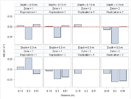
Calibration results showed values of RMSE and ME between simulated and measured soil-water content ranged from 0.012 to 0.091 m3 m-3, and -0.08 to 0.057 m3 m-3, respectively indicating that the simulations agree reasonably well with the measured data. The extreme values of RMSE and ME were occurred at locations occupied by the root zone 0.30 m from the dripline at both sensor depths. The coefficient of determination (r2) ranged between 0.7 and 0.56 at locations 0.15 and 0.50 m from the dripline, respectively.

The modeling of different SDI design configurations predicted that dripline spacing, dripine depth, and irrigation treatment had pronounced effects on T/Tp. Emitter spacing

(dripline flow rate) had no significant effect on T/Tp. An irrigation treatment of 100% peak

daily ETc provided greater amounts of water available for transpiration than 75% peak daily

ETc. With the same amount of irrigation water, transpiration was greater at a dripline spacing

(3)

(4)

Numerical Simulation of Soil-Water Distribution and Root Uptake from Subsurface Drip Irrigation Considering its Design and Management Parameters Using Hydrus-2D

by Vireak Kong

A thesis submitted to the Graduate Faculty of North Carolina State University

in partial fulfillment of the requirements for the degree of

Master of Science

Biological and Agricultural Engineering

Raleigh, North Carolina

2014

APPROVED BY:

_______________________________ ______________________________ Dr. Rodney L. Huffman Dr. Joshua L. Heitman

________________________________ Dr. Garry L. Grabow

(5)

ii

DEDICATION

(6)

iii

BIOGRAPHY

Vireak Kong was born in Kampong Thom, Cambodia, to Chanty Kong and Samnang Toun. Vireak has a sister, Chakrya Kong. Vireak realized his interest in science when he realized he was better at mathematics in high school. Vireak realized his appreciation for agricultural landscapes when his parents took him and his sister on trips to countryside annually during high school summer break. Agricultural landscapes there are beautiful and pristine. There, Vireak would walk rice paddy dams or ride wooden canoes along canals with some of his relatives.

(7)

iv

ACKNOWLEDGMENTS

I would like to express my sincere gratitude to my advisor, Dr. Garry Grabow for your invaluable time, guidance, thoughtfulness, and patience throughout the program. Thank you for your support to travel to the conference. Your research rigor and enthusiasm are contagious, keeping me motivated to go through critical times. Your writing rigor has always helped me have a better writing skill. You always found good solutions for me when I

encountered challenges or inadvertently made mistakes. Thank you for your understanding. Without your guidance, extensive reviews, and edits, I never would make this thesis a reality. Your feedback and constructive criticism are uplifting and have always helped me grow as a student and a person, and they will always stay inside me throughout my life. Thank you for everything you have done for me.

My appreciation also goes to my other committee members, Dr. Rodney Huffman and Dr. Joshua Heitman, for your contribution to this research project. Dr. Huffman, I was

impressed with your words of wisdom. I was particularly fascinated with ‘swim or drown’ and the examples you provided. Dr. Heitman, thank you for kindly providing the Hydrus-2D software for me to use for this research. Thank you to Dr. Jason Osborne for the statistical model guidance. Thank you to Dr. Ronnie Heiniger for corn production information. Thank you to Dr. Dan Willits for the research seminars. And, thank you to the department of Biological and Agricultural Engineering for the friendly atmosphere.

(8)

v

LIST OF TABLES

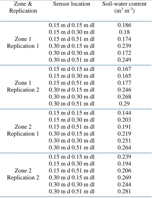
Table 2.1. Observed initial soil volumetric water content at sensor locations. ... 54

Table 2.2. Soil particle distribution, USDA classification, saturated hydraulic conductivity, and soil-water content at five levels of pressure from soil cores obtained near sensor locations of the field. ... 55

Table 3.1. Annual reference evapotranspiration ETo (mm) from 1982-2013 generated by

Ref-ET (Allen, 2003). ... 97

Table 3.2. Calculated irrigation durations and Hydrus-2D variable flux in regard to dripline spacing and emitter spacing. ... 98

Table 3.3. Simulation scenarios derived from varying levels of different factors: Dripline depth, dripline spacing, dripline flow rate, irrigation treatment, and soil type. ... 99

Table 3.4. Corn growing degree days (GDD) for the 2008 corn growing season for Salisbury for a planting date of 11 April... 100

Table 3.5. Corn growing degree days (GDD) for the 2008 corn growing season for Kinston for a planting date of 5 April... 102

(12)

ix

LIST OF FIGURES

Figure 2.1. Locations of the soil-water sensors in the soil profile (cross-section view) used to

measure soil-water content. Figure not to scale. ... 56

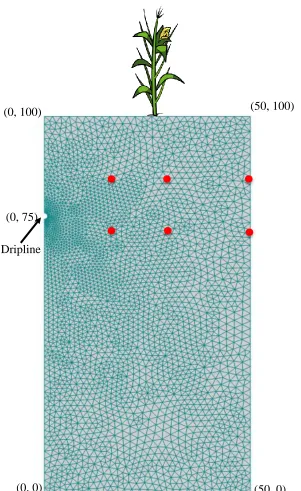
Figure 2.2. Domain geometry and generated unstructured finite element mesh for Hydrus-2D simulations. Coordinates in cm. ... 57

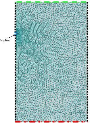
Figure 2.3. Boundaries used for Hydrus-2D simulations. ... 58

Figure 2.4. Normalized root distribution used for Hydrus-2D. ... 59

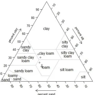
Figure 2.5. USDA triangle soil texture for Trebloc loam soil at study location. ... 60

Figure 2.6. Soil-water release curve for Trebloc loam soil at study location. ... 61

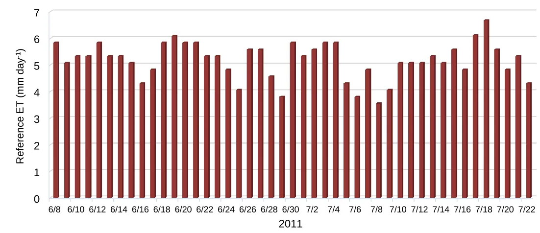
Figure 2.7. Daily reference evapotranspiration (mm day-1) for the simulation period from 8 June to 22 July 2011. ... 62

Figure 2.8. Basal crop coefficient (Kcb) for field corn using growth stage durations of 20, 35, 40 and 20 days for initial, crop development, midseason, and late season respectively using the daily dual crop coefficient procedure from Allen (1998). ... 63

Figure 2.9. Crop evapotranspiration (ETc), transpiration (Tp) and soil evaporation (E) from 8 June to 22 July 2011. Crop evapotranspiration was calculated using the dual crop coefficient method... 63

Figure 2.10. Mean bias Error (ME) for measured and modeled soil-water data by depth and distance from the dripline for both SDI zones and replications... 64

(13)

x Figure 2.12. Time series of simulated and measured soil-water data at 0.15-m depth 0.15 m from the dripline during the simulation period from day of the year (DOY) 159 to DOY 203 (8 June to 22 July 2011). ... 66

Figure 2.13. Measured soil-water data vs. simulated soil-water content at 0.15-m depth 0.15 m from the dripline. ... 67

Figure 2.14. Time series of simulated and measured soil-water data at 0.30-m depth 0.15 m from the dripline during the simulation period from day of the year (DOY) 159 to DOY 203 (8 June to 22 July 2011). ... 68

Figure 2.15. Measured soil-water data vs. simulated soil-water content at 0.30-m depth 0.15 m from the dripline. ... 69

Figure 2.16. Time series of simulated and measured soil-water data at 0.15-m depth 0.50 m from the dripline during the simulation period from day of the year (DOY) 159 to DOY 203 (8 June to 22 July 2011). ... 70

Figure 2.17. Measured soil-water data vs. simulated soil-water content at 0.15- and 0.30-m depth 0.51 m from the dripline during the simulation period from day of the year (DOY) 159 to DOY 203 (8 June to 22 July 2011). ... 71

Figure 3.1. Monthly average daily reference evapotranspiration (1997-2013) compared with the simulated year, 2008 in (a) Kinston and (b) Salisbury, NC. ... 105

Figure 3.2. Domain geometry and normalized root distribution used for Hydrus-2D

simulations. Coordinates in cm. ... 106

Figure 3.3. Domain geometry and normalized root distribution used for Hydrus-2D.

(14)

xi Figure 3.4. Distribution of T/Tp by dripline spacing, dripline depth, irrigation treatment, and

emitter spacing. ... 108

Figure 3.5. Distribution of T/Tp by dripline depth*dripline spacing. ... 109

Figure 3.6. Distribution of T/Tp by dripline spacing*irrigation treatment. ... 109

Figure 3.7. Distribution of T/Tp by dripline depth*irrigation treatment. ... 110

(15)

1

CHAPTER 1. REVIEW OF LITERATURE

Introduction

Recent droughts have caused interest in efficient irrigation and water management in agriculture. Efforts are being made to produce more food using less water and without degrading water and soil resources. One of the latest and most advanced methods of

irrigation, subsurface drip irrigation (SDI), has proven to be an example of efficient irrigation technology to meet this challenge with the expansion of this practice in the United States. The latest USDA Farm and Ranch Irrigation Survey (USDA-NASS, 2009) reported that the area covered by SDI in the U.S. has jumped from 163,000 to 260,000 ha in the five-year period 2003 to 2008, an increase of 59%.

SDI is compatible with small irregularly-shaped fields commonly found in the southeastern U.S. and has a competitive advantage over pivot and other overhead irrigation methods in these cases (Grabow et al., 2006; Bosch et al., 1998; O’Brien et al., 1998). SDI presents further opportunities for improving water use efficiency by reducing losses to evaporation by not relying on the soil surface for water transmission, all the while improving crop yields (Camp, 1998). Camp (1998) reported that in many cases SDI produced greater or equal crop yields than other irrigation methods and in most cases used less water.

(16)

2 Benefits of Sub-Surface Drip Irrigation (SDI)

Camp and Lamm (2003) defined SDI generally as water application below the soil surface with discharge rates in the same range as drip emitters. The driplines are beneath the surface, and water, nutrients, and pesticides are supplied to the plant’s root zone while keeping the soil surface dry. Camp (1998) and Lamm (2002) asserted that drip emitters in SDI systems buried in the soil help to minimize soil evaporation and runoff, conserve water, facilitate heavy trafficability in the field, and elevate longevity of driplines and emitters. Benefits of SDI can be realized in three areas: water and soil, cropping and cultural practices, and system infrastructure (Lamm, 2002).

Advantages pertaining to water and soil may include more efficient water use, improved opportunities for use of degraded waters and greater water application uniformity (Lamm and Camp, 2007; Lamm, 2002). SDI greatly reduces soil evaporation, surface runoff, and deep percolation by efficiently distributing water within the root zone (Lamm and Camp, 2007). A lysimeter study done by Phene et al. (1989) found that SDI reduced soil evaporation by 50% and 75% compared with high and low frequency surface drip respectively. Lamm and Trooien (2002) found that SDI could reduce irrigation water use for corn production by 35% to 55% compared to traditional irrigation methods such as center pivot.

SDI can enhance plant growth, crop yields and quality, boost plant health, and improve fertilizer and pesticide management (Lamm, 2002). Careful management of SDI systems irrigating corn eliminated 25% of irrigation needs while still maintaining top yields of 2.85 Mg ha-1_{(Lamm et al., 1995). Alam et al. (2002) showed that a well-designed SDI}

(17)

3 Advantages related to system infrastructure include ease of automation, decreased energy costs, design flexibility, and less pest damage (Lamm, 2002). Due to being conducive to system automation, SDI is highly likely to avoid over-irrigation, which causes nutrient leaching, and soil surfacing, and under-irrigation, which results in crop stress and thus yield reduction. Automation of irrigation systems based on soil moisture sensors may further improve water use efficiency (Shae et al., 1999).

Automated SDI Systems

Generally, two approaches have been used for irrigation scheduling. One method called “checkbook” involves estimating crop water needs based on evapotranspiration,

rainfall, and irrigation. The other approach directly measures soil-water via measurement devices such as neutron probes, granular matric sensors (GMS), or time domain reflectory (TDR). Automated irrigation control is adapted from this approach as automated irrigation control involves using feedback from the soil-water content measurement devices, rain gauges, etc., to schedule irrigation.

In a study done on corn, Caldwell et al. (1994) used a neutron probe to measure soil-water content in order to schedule the irrigation treatment. The authors found that time-based irrigation of seven days and depletion-based SDI produced less drainage under the root zone and higher water use efficiency than more frequent irrigation.Grabow et al. (2004), Meron et al. (1996), and Muñoz-Carpena et al. (2005) used GMS to control SDI and drip irrigation systems using soil-water feedback. Dukes and Scholberg (2004) found SDI irrigation water savings of 23% and 50% by using TDR and commercially available dielectric sensors compared to sprinkler treatments on sweet corn and bell pepper, respectively.

(18)

4 over the previous 24 hours. Corn yield for SDI was not statistically different from yields under sprinkler irrigation, but significantly higher than a non-irrigated treatment. For soybean, no statistical differences were found for either yields or water use efficiency for SDI, sprinkler, and non-irrigated treatments.

While sensor-controlled SDI automation can lead to water savings, care must be taken with the selection of dripline depth and dripline spacing, so that yields can be

optimized while keeping initial costs down. Wider dripline spacing will lower material and installation cost, but that must be balanced against the system’s and soil’s capabilities of transmitting adequate water to the root zone. There are many factors to consider when selecting dripline spacing, dripline depth, and emitter spacing in the SDI design process. Soil texture, anticipated marketable yields, and crops to be grown (Bosch et al., 1998) are strong factors to determine SDI configurations. As noted by Lamm et al. (2012), a choice of dripline depth and dripline spacing with regard to soil type is one of the big challenges facing growers considering SDI. Therefore, comparisons of relative differences in crop yield and water use efficiency as effected by dripline spacing, dripline depth, and emitter spacing have often been evaluated, specifically on corn (Grabow et al., 2011; Abat et al., 2010), cotton (Grabow et al., 2006; Camp et al., 1997), and sweet corn (Duke and Scholberg, 2004).

SDI Spacing and Depth Impact on Yield and Water Use Efficiency

(19)

5 1.83 (alternate row middles), and 2.74 m (under every third row), Powell and Wright (1993) found that average corn yields were 100%, 93%, and 94% of maximum.

In a study by Grabow et al. (2011), there was no difference in corn grain yield

between dripline spacings of 1.52- or 2.28 m or between either dripline spacing and sprinkler irrigated grain yield. Camp et al. (1997) evaluated 1.0- and 2.0-m dripline spacings for cotton in the Southeastern Coastal Plain and found that the cotton lint yield did not differ between dripline spacings in any study years. In a study done in a sandy soil common to Florida, Dukes and Scholberg (2004) found that dripline placed 0.33-m deep SDI was too deep for optimal corn yields while similar yields were found between 0.23-m deep SDI and sprinkler irrigation, but 0.23-m deep SDI reduced water use 11%. In a study done in a silt loam soil of Great Plains, Arbat et al. (2010) found that emitter spacings of 0.30 to 0.60 m resulted in no difference in corn yield and water use efficiency. Grabow et al. (2006) reported no difference on seed cotton yield and irrigation water use efficiency between dripline spacings of 0.91 and 1.82 m.

In a study done in Georgia, Sorensen et al. (2001b) found that SDI resulted in 38% more yield for peanut compared to non-irrigated treatments, but there was no difference in yield due to dripline spacings, amount of irrigation water applied, or emitter spacing. In a four-year yield study to examine the effects of dripline depth, Lamm and Trooien (2005) reported that yields were slightly less for the deepest (0.61 m) dripline depth and crop water use slightly less was for the 0.51- and 0.61-m depths compared to the 0.20-, 0.30-, and 0.41-m depths. Enciso et al. (2005) looked at the econo0.41-mics of different dripline depths for cotton on a clay loam soil and found that the 0.30-m dripline depth had greater yields and net returns than the 0.20-m dripline depth. Dripline depth for SDI systems generally ranges from 0.02 to 0.70 m (Camp, 1998).

(20)

6 spacing and dripline depth decisions are site and crop system specific. Adequate SDI designs and management have been defined as “the judicious combination of dripline spacing, emitter flow rate, and irrigation duration” (Provenzano, 2007). For SDI designs to be practical, dripline spacing must be a compromise between being wide enough to be financially feasible and narrow enough to provide sufficient amounts of water in the root zone. Dripline depth must be deep enough for cultural practices such as disking, and shallow enough for sufficient water to reach the upper root zone without excessive wet soil

evaporation. Modeling differently configured systems may provide insight into SDI configurations and management practices. Soil-water distribution obtained from modeling can be a benchmark for evaluating systems. Of the above studies in this section, only Grabow et al. (2006, 2011) investigated soil-water distribution from SDI and provided formal

statistically-based conclusions on how soil-water distributed between dripline spacing and dripline depth.

SDI and Soil-water Distribution Effects

An investigation on soil-water distribution from SDI systems is very crucial in predicting the success of system design (Grabow et al., 2006; Elmaloglou and

Diamantopoulos, 2009) as it impacts irrigation scheduling and water use efficiency. However, little research has been conducted on soil-water distribution under SDI systems with most of researchers evaluating only the impact of SDI dripline spacing on crop yields.

Singh et al. (2006) used dimensional analysis to fit a model that predicts the width and depth of wetted volume from discharge and irrigation duration and dripline depth. The authors found that wetting depth increased with dripline depth at all discharge rates

(21)

7 An investigation of soil-water distribution by Grabow et al. (2006) indicated that there was no difference in the extent of lateral water movement between dripline spacings of 0.91 and 1.82 m in a coastal plain soil for cotton. In a study done in a piedmont clay soil, water from the dripline typically spread laterally from the dripline a distance greater than 0.38 m but less than 0.78 m (Grabow et al., 2011).

Computer modeling has also been used to study SDI soil-water distribution. Cote et al. (2003) simulated soil-water distribution from SDI with a 0.30-m dripline depth for different soil types using Hydrus-2D. The simulation results showed downward water

movement and water not reaching the soil surface on a sandy soil, spherical water movement on a silt soil, and little deep percolation in a layered soil.

Application rate, soil type, root water uptake pattern and root distribution, dripline depth, emitter spacing, and irrigation scheduling all impact the vertical and lateral movement of water. As soil-water movement patterns under SDI play a pivotal role in deciding the efficacy of SDI configurations, it is important that soil-water content be accurately measured to assess different SDI configurations. Methods of soil-water estimation range from simple and direct gravimetric measurement procedures to sensors to computer simulations capable of predicting soil-water content over time and space. Therefore, choosing a tool that can accurately predict soil-water distribution is important for development of SDI management strategies and installation guidelines.

Soil-Water Distribution Evaluation Methods

(22)

8 gravimetric determination of soil-water content is time consuming and destructive, rendering it impractical for most purposes other than sensor calibration.

Others have used soil pits for measurement of wetting front advance (Battam et al., 2003; and Skaggs et al., 2004). The disadvantages of soil pits are lower accuracy and system perturbation (i.e. system changes once it is disturbed). Consequently, alternate methods are needed to provide a quick and reliable tool in assessing soil-water content.

Alternatively, Grabow et al. (2006) used an empirical statistical model with measured soil-moisture to test for differences in soil-water content at different distances from the dripline. In this method, the authors used GMS to measure soil-water tension and converted tension to volumetric soil-water content using a soil-water release curve developed from soil cores, to understand water movement and extraction between different SDI dripline spacing. TDR measurements were used by Dukes and Scholberg (2004) as feedback to automate an SDI system. These methods, however, are costly (requiring many sensor devices and installation), time consuming, and laborious (Patel and Rajput, 2008) with accuracy subject to sensors coverage. Soil-water distribution modeling under SDI has captured the attention of researchers (Van Bavels et al., 1973; Mmolawa and Or, 2003; Skaggs et al., 2004;

Lazarvoitch et al., 2005; Singh et al., 2006).

Empirical modeling is another method to understand soil-water distribution. Schwartzman and Zur (1986), Singh et al. (2006), and Kandelous et al. (2008) developed empirical models for estimating lateral, and vertical soil-water distribution. Kandelous and Simunek (2010) subsequently found that the empirical model could not provide a good description of the wetting pattern unless the conditions were similar to those for which it was developed.

Analytical modeling is one of the tools used to model soil-water distribution.

(23)

9 “WetUp” as an analytical tool to understand the SDI wetting pattern from drippers.

Mmolawa and Or (2000) developed a two-dimensional analytical model to describe soil-water distribution under transient flow conditions with the presence and absence of plant uptake and found good agreement with measurements of water and solute uptake. The authors also discovered that without plant uptake the analytical model accurately predicted soil-water dynamics from a point source. A major handicap of analytical models is that they often contain many simplifying assumptions pertaining to the linearization of the flow equation (Li et al., 2005) that may not effectively represent the observed reality in drip irrigation management (Kandelous and Simunek, 2010).

Numerical models such as Hydrus-2D (Simunek et al., 1999) are fast and inexpensive methods to simulate water movement for surface and subsurface drip irrigation and have become effective tools for use in SDI soil-water distribution research. Hydrus-2D (Simunek et al., 1999) is a well-known windows-based computer software package used for simulating water, heat, and solute movement in two-dimensional variably-saturated porous media. Hydrus-2D uses the Richards equation for variable flow through which soil-water content can be determined at very small time steps at very fine vertical and lateral resolution. There are many benefits of using Hydrus-2D for modeling soil-water movement including its sound physical basis, its relatively inexpensive cost, and the ability to run many simulations

(24)

10 Hydrus-2D Governing Equation and Input Requirements

Hydrus-2D was developed at the U.S. Salinity Laboratory, Agricultural Research Station, Riverside, California. Hydrus-2D can be used to simulate infiltration, evaporation, root water uptake (transpiration), soil-water storage, deep drainage, groundwater recharge, and lateral flow (Simunek et al., 2012).

The package consists of the SWMS-2D code (Simunek et al., 1994) for simulating water flow, heat, and solute movement in two-dimensional, variably-saturated media. The program numerically solves the Richards equation for the governing water flow using Galerkin-type linear finite element schemes. The flow equation consists of sink terms for water uptake by plant roots as a function of both water and salinity stress. Water uptake by roots is assumed to be zero close to saturation. The Richards equation was derived from the continuity equation and Darcy flux.

The mass balance can be written in two dimensions as:



 



or,

in out in out

q q q q

t x z

q q

t x z



   



 

  

 _{ } _

  



(1.1)

where

θ = volumetric water content (L3 _L-3₎

qin ∆𝑥∆𝑧 qout ∆𝑥∆𝑧

∆𝑥

(25)

11

q = water flux (L T-1)

t = time (T)

x = horizontal space coordinate

z = vertical space coordinate.

Horizontal and vertical water flux can be defined by Darcy’s law as:

x z H q K x H q K z         (1.2) where

K = hydraulic conductivity (L T-1)

H = hydraulic head (L).

Substituting equation 1.2 into equation 1.1 yields as:

K H K H

t x x z z



 _    _    

   

  _  _  _  _ (1.3)

Substituting for H=h+z (where h is the pressure head and z is the position head) for the vertical direction yields as:

K h( ) h K h( ) h K h( )

t x x z z



 _    _    _ 

   

         (1.4)

A sink term, S(h) (T-1), is introduced in the flow equation for water uptake by plant roots as a function of both water and salinity stress. Equation 1.4 becomes:

K h( ) h K h( ) h K h( ) S h( )

t x x z z



 _    _    _ _

   

  _  _  _  _ (1.5)

(26)

12 The term 𝑆(ℎ) represents the volume of water removed per unit time from a unit volume of soil due to plant water uptake. Feddes et al. (1978) defined 𝑆(ℎ) as:

S h

( )





( )

h S

_p (1.6)

where

α(ℎ)= the water stress response function of the soil-water pressure head (0≤ α ≤1) (L-1₎

Sp = the water uptake rate during periods of no water stress whenα(ℎ) = 1.

When the potential water uptake rate is equally distributed over a two-dimensional rectangular root domain, Sp becomes:

p 1 t p x z

S S T

L L

 (1.7)

where

Tp = the potential transpiration rate (L T-1),

Lz = the length of the root zone (L),

Lx = the width of the root zone (L),

St = the width of the soil surface associated with the transpiration process (L).

Equation 1.7 may be generalized by introducing a non-uniform distribution of the potential water uptake rate over a root zone of arbitrary shape (Vogel, 1988):

S_p b x z S T

 

, _t _p (1.8)

The actual water uptake distribution is then obtained by substituting equation 1.8 into equation 1.6:

(27)

13 where, 𝑏(𝑥, 𝑧) denotes the dimensionless spatial distribution of unstressed root water uptake

(L2_L-2_{). This function describes the variation of the potential extraction term, 𝑆}

𝑝, over the root zone. For the non-uniform cases, Vrugt et al. (2001) defined 𝑏(𝑥, 𝑧) as:

* *

( , ) 1 1

z r

m m

p p

z z r r

z r

m m

z r

b r z e

z r                        __  _{ }_  _    

  (1.10)

where

rm = the maximum rooting length in the horizontal direction (L)

zm = depth direction (L)

pz, z*, pr and r*= empirical parameters that can describe non-symmetrical root

geometries.

Soil Hydraulic Parameter Requirements for Hydrus-2D

Hydrus-2D requires initial water content distribution and the van Genuchten soil hydraulic parameters (i.e. a soil-water release curve and hydraulic conductivity). These are important in investigating water flow. Soil water release curve parameters may be obtained using suction and pressure plate procedures on field cores (Grabow et al., 2006; Grabow et al., 2011). Alternatively, these parameters may be obtained from Rosetta (Schaap et al., 2001) using soil physical properties (Skaggs et al., 2004).

The van Genuchten functions (van Genuchten, 1980) for water retention and hydraulic conductivity are defined as:

 



1



0 0

s r

r _n m

s h h h h            _      (1.11)





2 1/

( ) s el 1 1 em m

K h K S _  S _

(28)

14 and

r , 1 1

e

s r

S m

n

   



  

 (1.13)

where

θs = the saturated volumetric water content (L3 L-3) θr = the residual water content (L3 L-3)

Ks = the saturated hydraulic conductivity (L T-1)

l = pore size distribution

Se = effective water content (L3 L-3)

α = empirical constant (L-1₎

m, n = empirical constant with m= 1-1/n, and h = pressure head (L). The empirical constants are fitting parameters that define the shape of the curve.

Root Distribution and Root Water Uptake

Plant root distribution is one of the most important processes in modeling subsurface water flow and solute dynamic. Root water uptake (and soil-water distribution pattern) interactively determine the success of SDI design and management strategies. Root water uptake is equivalent to water lost by plant transpiration. Sufficient irrigation water must be applied to the root zone to provide enough water to the plant to prevent plant stress, as inadequate water results in plant stress and reduced root water uptake. Therefore, root water uptake is a strong surrogate to infer the success of SDI design, installation, and management strategies.

(29)

15 rate than the plant can uptake (Gardenas et al., 2005). The amount of irrigation water

supplied to meet crop water demands can be applied in several fashions. Irrigation can be set to fully and partially replace daily evapotranspiration in a daily or every other day basis. Each irrigation regime or strategy will result in a different soil-water distribution pattern, thus yielding different root distribution and root water uptake (Gitz, 2006).

Clothier and Green (1994) reported that knowledge of crop root distribution and water uptake pattern is essential to matching irrigation system design and management with crop requirements. Gardenas et al. (2005) claimed that water uptake by plant roots

determines spatial and temporal patterns of available soil-water. In an attempt to aid drip irrigation design, Coelho and Or (1996) expanded the plant uptake function by fitting a function better describing temporal and spatial change in uptake intensity.

In a study done on alfalfa, Kandelous et al. (2012) used Hydrus-2D to model soil-water distribution and concluded that root distribution has a large effect on optimal applied irrigation water, irrigation water scheduling, and deep percolation loss. Coelho and Or (1999) added that irrigation scheduling schemes that depend on monitoring soil-water status must take root water extraction patterns into account. Coelho and Or (1999) used TDR sensors to measure water uptake at high spatial and temporal distribution. Potential factors affecting root system patterns include spatial and temporal variations in soil-water availability and soil matric potential (Feddes et al., 1976; Michelakis et al., 1993). These factors can be solved in Hydrus-2D, which simulates two-dimensional axially symmetric water flow and root water uptake based on finite element numerical solutions of the flow equations (Simunek et al., 1999).

Model Calibration

(30)

16 management strategies). Model calibration is needed when simulated characterizations for a particular problem are different from those to which it was intended. Hydrus-2D may work well for one field site, but it may not work equally well for other sites. Another motivation for model calibration is when some input parameters are missing or not independently measured. Found in Simunek et al. (2012), Simunek and Hopmans (2002) defined model calibration as the process of fitting within reasonable ranges the input parameters (e.g. soil hydraulic parameters or root water distribution) and initial or boundary conditions of a model for a particular problem until the simulated model results and the observed or measured variables (e.g. pressure heads, water content, concentrations, various fluxes) closely match. As the definition dictates, the success of model calibration is when the measured data and the outputs produced are within some acceptable level of precision and accuracy.

There are two steps in the calibration process. The first step involves using the existing data to calibrate the model and to estimate all necessary input parameters while the second validation process compares simulated and measured data outputs using the estimates of parameters calibrated found in the first process (Simunek and de Vos, 1999). The second process determines the success of model calibration such that the model responses are within acceptable ranges of accuracy. This two-process calibration is often hailed as historical validation (Simunek et al., 2012). Hydrus-2D calibration has been carried out in many studies. For example, Bufon et al. (2012) found that Hydrus-2D simulations of volumetric soil-water content were accurate within ±3% when compared to measured values obtained

with TDR probes using a soil-specific calibration. The authors suggested that the model be used to evaluate irrigation strategies. Kool et al. (2014) used Hydrus 2D/3D to predict hourly evapotranspiration and found that the predictions compared well with measured data.

(31)

17 agreement between simulated and gravimetrically obtained soil-water data. This result, showing that Hydrus-2D can be a relatively powerful tool for designing and investigating drip irrigation management practices, is similar to that reported by Ben-Gal et al. (2004), Provenzano (2007), and Li et al. (2005).

Hydrus-2D is a physically based model and thus needs no calibration when all required input parameters (i.e. soil hydraulic parameters for water flow) are independently determined (Simunek et al., 2012), and simulated conditions for a particular problem are as those to which it was intended. However, input parameters are difficult to measure. There is little evidence in the literature in which all required input parameters have been

independently determined. As noted by Simunek et al. (2012), in most applications one or two parameters required by the model may be lacking. That is, Hydrus-2D requires calibration in almost all situations in which it is first used.

Estimation of Soil Hydraulic Properties

Hydrus-2D needs soil hydraulic properties for its primary input. Two methods may be used to determine soil hydraulic properties: laboratory and in situ measurements. Hydrus-2D has code for estimating soil hydraulic parameters as per calibration. Soil hydraulic

parameters can be estimated by a catalog of average parameters for 12 textural classes of the USDA textural triangle (Carsel and Parrish, 1988) or pedotransfer functions (Schaap et al., 2001) using the Rosetta program. Rosetta is a pedotranser function software package that uses a neural network model to estimate hydraulic parameters from soil texture and related data such as bulk density. Skaggs et al. (2004) estimated soil hydraulic parameters by Carsel and Parrish estimates (Carsel and Parrish, 1988), and full Rosetta, and found that the

predictions with Rosetta matched with the measured data more closely than the data obtained with Carsel and Parrish estimates. Field data or laboratory measurements can be used

(32)

18 Review of SDI Research using Hydrus-2D

Although an increase in SDI research has occurred recently (Lamm et al., 2012), the literature generally lacks good information on how dripline spacing and dripline depth affect both lateral and vertical movement of water. Comprehensive knowledge of this is necessary to develop SDI installation guidelines and irrigation strategies that growers could use to obtain high yields. Examining all possible placement of the drip tape and all possible SDI scheduling strategies through field experiments requires extensive time and sizeable

resources. However, numerical simulation models, such as Hydrus-2D, can be used to predict the soil-water distribution for different ranges of dripline spacing, dripline depth, and

irrigation strategies in a fast and inexpensive fashion. However, little work has been done to justify that the model can be used to develop design guidelines and irrigation management strategies. Furthermore, Hydrus-2D has not been calibrated under SDI cropping systems and dripline spacings and depths found in North Carolina.

Research Objectives

The primary objectives of this study were to:

(33)

19

REFERENCES

Ajdary, K., Singh, D.K., Singh, A.K., and Khanna, M. 2005. Simulation of water distribution under drip irrigation using Hydrus-2D. In: XII World water Congress Water for Sustainable Development—Towards Innovative Solutions, 22–25 November 2005, New Delhi, India, pp. 221–231.

Alam, M., Trooien, T. P., Dumler, T. J., and Rogers, T. H. 2002. Using subsurface drip irrigation for alfalfa. J. Am. Water Res. Assoc. 38(6): 1715–1721.

Arbat, G. P., Lamm, F. R., and Abou Kheira, A. A. 2010. Subsurface drip irrigation emitter spacing effects on soil-water redistribution, corn yield, and water productivity. Appl. Eng. in Agric. 26(3): 391-399.

Battam, M. A., Sutton, B. G., and Boughton, D. G. 2003. Soil pits as a simple design aid for subsurface drip irrigation systems. Irrig. Sci. 22(3-4): 135-141.

Ben-Gal, A., Lazarovitch, N., and Shani, U. 2004. Subsurface drip irrigation in gravel-filled cavities. Vadose Zone J. 3: 1407–1413.

Bhattarai, S. P., Pendergast, L., Midmore, D. J. 2006. Root aeration improves yield performance and water use efficiency of tomato in heavy clay and saline soils. Sci Hort. 108(3): 278–288.

Bosch, D. J., Powell, N. L., and Wright, F. S. 1998. Investment return from three subsurface micro irrigation tubing spacings. J.Prod. Agric. 11(3): 370-376.

(34)

20 Caldwell, D. S., Spurgeon, W. E., and Manges, H. L. 1994. Frequency of irrigation for

subsurface drip irrigated corn. Trans. ASAE 37(4): 1099-1103.

Camp, C. R. 1998. Subsurface drip irrigation: A Review. Trans. ASAE 41(5): 1353-1367.

Camp, C. R., Bauer, P. J., and Hunt, P. G. 1997. Subsurface drip irrigation lateral spacing and management for cotton in the southeastern coastal plain. Trans. ASAE 40(4): 993-999.

Camp, C. R., Baucer, P. J., and Busscher, W. J. 1999. Evaluation of no-tillage crop production with subsurface drip irrigation on soils with compacted layers. Trans. ASAE 41(5): 1353-1367.

Camp, C. R., Garrett, J. T., Sadler, E. J., and Busscher, W. J. 1993. Microirrigation management for double-cropped vegetables in a humid area. Trans. ASAE 36(6): 1639–1644.

Camp, C. R., and Lamm, F. R. 2003. Irrigation Systems, Subsurface Drip. Encyclopedia Water Science. Marcel Dekker, New York, New York. pp. 560-564.

Carsel, R. F., and Parrish, R. S. 1988. Developing joint probability distributions of soil-water retention characteristics. Water Res. Res. 24(5): 755-769.

Clothier, B. E., and Green, S. R. 1994. Rootzone processes and the efficient use of irrigation water. Agric. Water Mgmt 25(1): 1-12.

Coelho, E. F., and Or, D. 1996. A parametric model for two dimensional water uptake by corn roots under drip irrigation. Soil So. Am. J. 60(4): 1039-1049.

(35)

21 Cook, F. J., Thorburn, P. J., Fitch, P., Charlesworth, P. B., and Bristow, K. L. 2006.

Modeling trickle irrigation: comparison of analytical and numerical models for estimation of wetting front position with time. Environ. Model. Softw. 21(9): 1353– 1359.

Cote, C.M., Bristow, K.L., Charlesworth, P.B., Cook, F.J., and Thorburn, P.J. 2003. Analysis of soil wetting and solute transport in subsurface trickle irrigation. Irrig. Sci. 22(3-4): 143–156.

Dukes, M. D., and Scholberg, J. M. 2005. Soil moisture controlled subsurface drip irrigation on sandy soils. Trans. ASABE 21(1): 89-101.

Elmaloglou, S., and Diamantopoulos, E. 2009. Simulation of soil-water dynamics under subsurface drip irrigation from line sources. Agric. Water Mgmt. 96(11): 1587-1595.

Enciso, J.M., Unruh, B.L., Colaizzi, P.D., and Multer, W.L. 2005. Economic analysis of subsurface drip irrigation lateral spacing and installation depth for cotton. Trans. ASAE 48(1): 197-204.

Feddes, R. A., Kowalik, P., Kolinska-Malinka, K. and Zaradny, H. 1976. Simulation of field water uptake by plants using a soil-water dependent root extraction function. J. Hydrol. 31(1-2): 13-26.

Gardenas, A.I., Hopmans, J.W., Hanson, B.R., and Simunek, J. 2005. Two-dimensional modeling of nitrate leaching for various fertigation scenarios under micro-irrigation.

Agric. Water Mgmt. 74(3): 219–242.

(36)

22 Grabow, G. L., Huffman, R. L., and Evans, R. O. 2011. SDI dripline spacing effect on corn

and soybean yield in a piedmont clay soil. J. Irrig. Drain. Eng. 137(1): 1943-4774.

Grabow, G. L., Huffman, R. L., Evans, R. O., Jordan, D. L., and Nuti, R. C. 2006. Water distribution from subsurface drip irrigation system and dripline spacing effect on cotton yield and water use efficiency in a coastal plain soil. Trans. ASABE 49(6): 1823-1835.

Grabow, G. L., Evans, R. O., Haman, D. Z., Sorensen, R. B., Ross, D. S., and Tacker, P. 2008. Critical management issues for SDI systems in North Carolina. North Carolina Cooperative Extension Service.

Hanson, B. R., Simunek, J., and Hopmans, J. W. 2006. Evaluation of urea-ammonium-nitrate fertigation with drip irrigation using numerical modeling. Agric. Water Mgmt. 86(1-2): 102–113.

Gitz, D.C., McMichael, B. L., Mahan, J. R., and Lascano, R. J. 2006. Effect of Alternate- Row Drip Irrigation Pattern on Cotton Root Distribution. In 2006 Beltwide Cotton Conference, San Antonio, TX. 03-06 Jan. 2006. Natl. Cotton Counc. Am., Memphis, TN.

Jiusheng, L., Zhang, J., and Ren, L. 2003. Water and nitrogen distribution as affected by fertigation of ammonium nitrate from a point source. Irri. Sci. 22(1): 19–30.

Kandelous, M. M., Liaghat, A., and Abbasi, F. 2008. Estimation of soil moisture pattern in subsurface drip irrigation using dimensional analysis method. J Agric. Sci. 39(2): 371–378.

(37)

23 Kandelous, M. M., Kamai, T., Vrugt, J. A., Simunek, J., Hanson, B., and Hopmans, J. W.

2012. Evaluation of subsurface drip irrigation design and management parameters for alfalfa. Agric. Water Mgmt. 109: 81-93.

Kool, D. Ben-Gal, A., Agam, N., Simunek, J., Heitman, J. L., Sauer, T. J., and Lazarovitch, N. 2014. Spatial and diurnal below canopy evaporation in a desert vineyard:

measurements and modeling. Water res. res. 50(8): 7035-7049. DOI: 10.1002/2014WR015409.

Lamm, F. R. 2002. Advantages and disadvantages of subsurface drip irrigation. In International Meeting on Advances in Drip/Micro Irrigation, Puerto de La Cruz, Tenerife, Canary Islands.

Lamm, F. R., Bordovsky, J. P., Schwankl, L., Grabow, G. L., Enciso-Medina, J., Peters, R. T., Colaizzi, P. D., Trooien, T. P., and Porter, D. O. 2012. Subsurface drip irrigation: Status of the technology in 2010. Trans. ASABE 55(2): 483-491.

Lamm, F. R., and Camp, C. R. 2007. Subsurface drip irrigation. Chapter 13 in

microirrigation for crop production design, operation and management. F.R. Lamm, J.E. Ayars, and F.S. Nakayama (Eds.), Elsevier Publications. pp. 473-551.

Lamm, F. R., Manges, H. L., Stone, L. R., Khan, A. H., and Rogers, D. H. 1995. Water requirement of subsurface drip-irrigated corn in northwest Kansas. Trans. ASAE

38(2): 441-448.

Lamm, F. R., and Trooien, T. P. 2005. Dripline depth effects on corn production when crop establishment is nonlimiting. Trans ASAE 21(5): 835-840.

(38)

24 Lazarvoitch, N., Simunek, J., and Shani, U. 2005. System dependent boundary condition for

water flow from subsurface source. Soil Science Society of America Journal 69: 46– 50.

Li, J., and Liu, Y. 2011. Water and nitrate distributions as affected by layered-textural soil and buried dripline depth under subsurface drip fertigation. Irrig. Sci. 29(6): 469–478.

Li, J., Zhang, J., and Rao, M. 2005. Modeling of water flow and nitrate transport under surface drip fertigation. Trans. ASAE 48(2): 627-637.

Mailhol, J.C., Ruelle, P., and Nemeth, I. 2001. Impact of fertilization practices on nitrogen leaching under irrigation. Irrig. Sci. 20: 139–147.

Meron, M., Hallel, R., Shay, G., Feuer, R., and Yoder, R. E. 1996. Soil sensor actuated automatic drip irrigation of cotton. In Evapotranspiration and Irrigation Scheduling, Proc. of the International Conference, eds. C. R. Camp and E. J. Sadler, 886−891. St.

Joseph, Mich.: ASAE.

Michelkis, N., Vougioucalou, E. and Clapaki, G. 1993. Water use, wetted soil volume, root distribution and yield of avocado under drip irrigation. Agric. Water Mgmt. 24(2): 119-131.

Mmolawa, K., and Or., D. 2000. Water and solute dynamics under a drip-irrigated crop: Experiments and analytical model. Trans. ASAE 43(6): 1597-1608.

(39)

25 Muñoz-Carpena, R., Dukes, M. D., Yuncong, C. L., and Klassen, W. 2005. Field comparison

of tensiometer and granular matrix sensor automatic drip irrigation on tomato. Hor. Techonology 15(3) 584-590.

O’Brien, D. M., D. H. Rogers, F. R. Lamm, and G. A. Clark. 1998. An economic comparison

of subsurface drip and center pivot sprinkler irrigation systems. Applied Eng. in Agric. 14(4): 391-398.

Patel, N., and Rajput, T. B. S. 2008. Dynamics and modeling of soil-water under subsurface drip irrigated onion. Agric. Water Mgmt 95(12): 1335-1349.

Phene, C. J., Davis, K. R., Hutmacher, R. B., and McCormick, R. L. 1987. Advantage of subsurface irrigation for processing tomatoes. Acta Hort. 200: 101–113.

Phene, C. J., McCormick, R. L., Davis, K. R., Pierro, J., and Meek, D. W. 1989. A lysimeter feedback system for precise evapotranspiration measurement and irrigation control.

Trans. ASAE 32(2): 477-484.

Philip, J.R. 1984. Travel-times from buried and surface infiltration point sources. Water Res. Res. 20(7): 990-994.

Powell, N.L., and Wright, F.S. 1993. Grain yield of subsurface microirrigated corn as affected by irrigation line spacing. Agron. J. 85(6): 1165-1170.

Provenzano, G. 2007. Using HYDRUS-2D simulation model to evaluate wetted soil volume in subsurface drip irrigation systems. J. Irrig. Drain. Eng. 133(4): 342–349.

(40)

26 Schaap, M. G., Leij, F. L., and van Genuchten, M. Th. 2001. ROSETTA: a computer

program for estimating soil hydraulic properties with hierarchical pedotransfer functions. J. Hydrol, 251: 163-176.

Schwartzman, M., and Zur, B. 1986. Emitter spacing and geometry of wetted soil volume. J Irrig Drain Eng. 112(3): 242–253.

Shae, J. B., D. D. and Gregor, B. L. 1999. Irrigation scheduling methods for potatoes in the Northern Great Plains. Trans. ASAE 42(2): 351-360.

Simunek, J., and de Vos., J. A. 1999. Inverse optimization, calibration, and validation of simulation models at the field scale. In Modeling of Transport Process in Soils at Various Scales in Time and Space, 431-445. J. Feyen and K. Wiyo, eds. Wageningen, The Netherlands: Wageningen Pers.

Simunek, J., and Hopmans., J.W. 2002. Chapter 1.7: Parameter optimization and nonlinear fitting”. In Methods of Soil Analysis: Part 1. Physical Methods, 139-157. J. H. Dane and G. C. Topp, eds. 3rd ed. Madison, Wisc.: SSSA.

Simunek, J., Sejna, M., and van Genuchten, M.Th. 1999. The HYDRUS-2D software pack-age for simulating two-dimensional movement of water, heat and multiple solutes in variably saturated media, version 2.0. Rep. IGCWMC-TPS-53, Int. Ground Water Model. Cent., Colo. Sch. of Mines, Golden, CO, p. 251.

Simunek, J., Sejna, M., and van Genuchten, M.Th. 2012. HYDRUS: Model use, calibration, and validation. Trans. ASABE 55(3): 1263-1276.

(41)

27 1.1. Research Report No. 132, U. S. Salinity Laboratory, USDA, ARS, Riverside, CA.

Singh, D. K., Rajput, T.B.S., Sikarwar, H.S., Sahoo, R.N., and Ahmed, T. 2006. Simulation of soil wetting pattern with subsurface drip irrigation from line source. Agric. Water Mgmt 83(1-2): 130–134.

Skaggs, T. H., Trout, T. J., Simunek, J., and Shouse, P. J. 2004. Comparison of HYDRUS-2D simulations of drip irrigation with experimental observations. J. Irrig. Drain. Eng. 130(4): 304-310.

Sorensen, R. B., Wright, F. S., and Butts, C. L. 2001b. Pod yield and kernel size distribution of peanut produced using subsurface drip irrigation. Appl. Eng. in Agric. 17(2): 165−169.

USDA-NASS. 2009. Farm and Ranch Irrigation Survey (2007). Vol. 3: Special studies. In Census of Agriculture. USDA, Washington D.C.: USDA.

Van Bavel, C. H. M., Ahmed, J., Bhuiyan, S.I., Hiller, E.A., and Smajastrla, A.G. 1973. Dynamic simulation of automated subsurface irrigation system. Trans. ASAE 16(6): 1095–1099.

van Genuchten, M. Th. 1980. A closed-form equation for predicting the hydraulic conductivity of unsaturated soils. Soil Sci. Soc. Am. J. 44(5): 892-898.

(42)

28

CHAPTER 2. CALIBRATION OF HYDRUS-2D TO MEASURED

SOIL-WATER DATA

Introduction

As concerns proliferate over limited water supplies in the United States, interest in the use of subsurface drip irrigation (SDI) over conventional irrigation is increasing. SDI is one of the high-performance irrigation technologies that can overcome the challenges of limited or restricted water supplies and has been implemented in arid and semi-arid regions for many years. Even in semi-humid to humid regions, where rainfall is significant, its implementation is increasing. Although SDI is a relatively new option to North Carolina producers, it is becoming more popular as producers learn of its many benefits (Grabow et al., 2008). The latest USDA Farm and Ranch Irrigation Survey (USDA-NASS, 2009) reported that the area covered by SDI in the U.S. has increased from 163,000 to 260,000 ha in the five-year period 2003 to 2008, an increase of 59%.

SDI is defined as “the application of water below the soil surface by microirrigation

emitters with discharge rates usually less than 7.5 L h-1” (Lamm et al., 2012; Lamm and Camp, 2007; ASAE, S526.2 2001). SDI has numerous potential advantages. SDI allows almost all portions of the field to be irrigated efficiently. Irrigation water is precisely

controlled by delivering to the root zone directly. SDI can maintain soil-water distribution at a level favorable to plant growth (Camp, 1998). The field surface remains dry, curtailing weed growth, when the driplines are placed deep enough.

These advantages of SDI can be realized through proper design and management with regard to site conditions and cropping systems (Lamm, 2002). One of the challenges

(43)

29 narrow enough to provide sufficient amounts of water in the root zone. Dripline depth must be deep enough for cultural practices such as disking, and shallow enough for sufficient water to reach the upper root zone without excessive wet soil evaporation. Modeling of different SDI configurations has the potential to improve installation and management guidelines.

A comprehensive understanding of the mechanism of SDI soil-water distribution in the soil profile is imperative for proper SDI design and management. Knowledge of soil-water distribution can be obtained from tools ranging from simple and direct gravimetric measurement procedures to soil-water sensors to computer numerical simulations capable of spatially and temporally predicting soil-water content. Choosing a tool that can accurately predict soil-water distribution is important to efficiently design and manage SDI systems.

Arbat et al. (2010) used gravimetric measurement to see the effects of emitter spacing on soil-water redistribution. A drawback of gravimetric determination is that limited soil-water distribution data can be obtained due to laborious and time-consuming work and its destruction to soils rendering it impractical for most purposes.

Grabow et al. (2006) used an empirical statistical analysis with measured

soil-moisture data from nests of granular matrix sensors to look at differences in soil-soil-moisture at different distances from the dripline. Kandelous et al. (2008) developed empirical models for estimating soil-water distribution. Cook et al. (2006) developed a user-friendly software, called “WetUp” (Cook et al., 2003), as an analytical tool to understand wetting patterns from

buried sources such as SDI. A major handicap of analytical models is that they often contain many simplifying assumptions pertaining to the linearization of the flow equation that may not effectively represent observed reality in drip irrigation management (Kandelous and Simunek, 2010; Li et al., 2005).

(44)

30 based computer software package used to simulate two dimensional water, pressure head, and solute movement in porous media. The program numerically solves the Richards

equation for saturated and unsaturated water flow. Multiple studies have used Hydrus-2D and found it useful for SDI soil-water distribution modeling. For instance, Cote et al. (2003) used Hydrus-2D to simulate both soil-water and solute movement under SDI. Kandelous and Simunek (2010) used Hydrus-2D to simulate wetting patterns and compared predictions by Hydrus-2D with field and laboratory data, WetUp, and empirical models. Provenzano (2007) also evaluated wetted soil volume under SDI using Hydrus-2D.

Model calibration is needed when conditions are not the same to those that are used to formulate the model. A model may work well for one field site, but it may not work equally well for other sites. Another reason for model calibration is when some input parameters are missing or not independently measured. Simunek and Hopmans (2002) defined model

calibration as the process of adjusting within reasonable ranges the input parameters (e.g. soil hydraulic parameters and root distribution) and initial or boundary conditions of a model for a particular problem until the simulated model results and the observed or measured variables (e.g., pressure head, soil-water content, concentration, various fluxes) closely match. A model is judged to be successfully calibrated when measured data and model output are within some acceptable level of precision (Simunek et al., 2012) or accuracy.

Physically based models such as Hydrus-2D often need little calibration, when all required input parameters (e.g. soil hydraulic parameters for water flow and root distribution) are independently determined (Simunek et al., 2012), and simulated conditions for a

(45)

31 There is little evidence in the literature of studies in which all required input

parameters have been independently determined. In most scenarios one or two parameters required by the model is missing (Simunek et al., 2012). Hydrus-2D has options to determine missing parameters. For example, when soil hydraulic parameters are lacking, users can use pedotransfer functions as obtained by Schaap et al. (2001) using their Rosetta program for estimating soil hydraulic parameters from soil textural properties. Rosetta can also be used in a combination with field-determined data to estimate soil hydraulic parameters for calibrating Hydrus-2D (Simunek et al., 2012). Comparison between predicted soil-water content by Hydrus-2D and field observed data has been carried out in some studies using some of input parameters estimated with the Rosetta program (Ben-Gal et al., 2004; Provenzano, 2007; Skaggs et al., 2004; Bufon et al., 2012).

Ben-Gal et al. (2004) compared observed data to simulated soil-water content and found that the simulated soil-water content obtained with Hydrus-2D closely matched observed values. Wang et al. (2013) validated Hydrus-2D by comparing predicted soil-water content under SDI with measured soil-water data from field experiments and found that there was good correspondence between simulations and field observations. Bufon et al. (2012) found that soil-water content from Hydrus-2D was accurate within ±3% when compared to

measured soil-water data obtained from TDR soil-water sensors. The authors used field measured soil data combined with the pedotransfer function Rosetta to estimate the van Genuchten soil hydraulic properties. Liu et al. (2013) used Hydrus-2D to predict the temporal variation of soil-water content in a drip irrigated cotton field and found that their Hydrus-2D predictions agreed well with the field observations. Skaggs et al. (2004) compared the Hydrus-2D simulations of water infiltration and redistribution from drip irrigation with a 0.06-m installation depth in a sandy loam soil with gravimetric samplings and found satisfactory agreement.

(46)

32 the Hydrus-2D model must first be tested with field data specific to intended scenarios (i.e. corn, NC soils, NC climate, etc.) to provide confidence for design and management use. Secondly, all required input data for any particular site is not likely to be found or

independently determined for simulation purpose. Usually, there are at least one or two input parameters or variables missing.

The primary objective of this study was to investigate the accuracy of Hydrus-2D in estimating soil-water distribution for SDI on a coastal plain soil. The model incorporated irrigation, soil evaporation, crop transpiration, precipitation, and root water uptake.

Materials and Methods Site Description

Hydrus-2D calibration required both input data for the model and measured soil-water data for comparison. Soil-soil-water content data during the period of irrigation from DOY 159 (8 June) to DOY 203 (22 July) 2011 were used in this study. The field site from which data for model calibration were obtained is located in the coastal plain near Rowland, North Carolina, coordinates 34°32′7″N 79°17′33″W, and elevation of 45 m above sea level. The dominant soil types at the field site is Nahunta very fine sandy loam, Aycock very fine sandy loam, and Trebloc loam (USDA Web Soil Survey, 2014)

The SDI irrigated area was divided into two irrigation zones: zone 1 (approximately 3 ha) and zone 2 (approximately 6 ha). Soil-water content data used for model assessments were measured by Echo EC-5 soil-water sensors (Decagon Devices, Inc. Pullman, WA). Sensor nests were located at 0.15- and 0.30-m depths 0.15, 0.30, and 0.51 m (mid-dripline) from the dripline in both zones. The layout of the soil-water sensors is shown in figure 2.1. There were two replications of the soil-water sensors in both zone 1 and zone 2, each

(47)

33 Numerical Simulation Using Hydrus-2D

Soil-water distribution below the soil surface was simulated using the computer modeling Hydrus-2D (Simunek et al., 2008). Hydrus-2D can simulate two dimensional variably-saturated water flow, heat movement, and transport of solutes. Hydrus-2D

numerically solves the Richards equation for variably-saturated water flow. The model also includes sink terms for root water uptake, which affect the spatial distribution of soil-water. In this study, the flow problem was considered to be a line source with water flow and distribution being a two-dimensional process.

The Richards equation is the governing equation solved for water flow in homogenous and isotropic soil:

 

h

 

h

 

K h K h K h S h

t x x z z



 _    _    _ _

   

         (1.14)

where

θ = volumetric water content (L3 _L-3₎ h = soil-water pressure head (L)

t = time (T)

x = horizontal space coordinate

z = vertical space coordinate

K = hydraulic conductivity (L T-1)

S(h) = root water uptake (T-1).

Soil hydraulic properties were modeled using the van Genuchten model (van

(48)

34 located at the edge of the rectangular domain as a 0.8-cm radius semi-circle, 0.25 m below the soil surface. The transport domain was discretized into 6114 triangular finite elements (3150 nodes) using an unstructured finite element. Observation nodes, as depicted in figure 2.2, were assigned at 0.15- and 0.30-m depths 0.15, 0.30, and 0.50 m from the dripline to coincide with the locations of the soil-water sensors.

Initial and Boundary Conditions

The boundaries for the Hydrus-2D model are shown in figure 2.3. A time-variable atmospheric boundary condition was used at the upper water flow boundary condition. The atmospheric boundary condition included fluxes of precipitation, evaporation (E) and potential transpiration (Tp). Water was assumed to evaporate at potential evaporation rates

when the soil surface was below a threshold value (hCritA) of -10000 cm H2O of pressure

head. At the bottom of the soil profile, a free drainage boundary condition was imposed. This boundary condition assumes a unit gradient along the lower boundary because the water table at this site was assumed to be deep enough to not influence root zone soil-water dynamics. A variable flux boundary was used at the dripline emitter. The water flux at the variable flux boundary was calculated based on the rated 0.91 L h-1 emitter discharge flow rate, the dripline circumference, and the emitter spacing:

1

1 )

) emitter discharge flow rate (L h 10

water flux (cm h

dripline circumference (cm) emitter spacing (m)



 _ _

 (1.15)

During water application, the dripline boundary was set to a constant water flux of 2.97 cm h-1_{. When irrigation ended, flux was set to zero. At both sides of the domain, a}

zero-flux boundary was imposed during and after irrigation due to symmetry (Skaggs et al., 2004).

(49)

35 soil-water content at 6 sensor locations for both replications of both zones was set equal to the measured soil-water content one hour prior to the start of simulations (table 2.1). Initial soil-water content was set equal between sensor midpoints in both horizontal and vertical dimensions, and for soil-water content at the domain edges was set equal to soil-water content measured by the closet sensor. From 0.40-m depth to the bottom of the domain, initial soil-water content was assumed to be at field capacity as plant extraction would be expected to be nil below this depth.

Parameters and Variable Inputs Soil Physical Properties

Hydrus-2D requires soil hydraulic parameters: 𝜃_𝑟, 𝜃_𝑠𝑎𝑡, 𝛼, 𝑛, 𝑙 for use in defining a

soil-water release curve, and Ksat. Undisturbed core soil samples were taken from the soil

profile to determine particle size distribution, bulk density, soil-water retention to develop a soil-water release curve. The samples were taken using cylindrical samplers 0.076 m in diameter and 0.076 m long. The soil cores were extracted at 0.15- and 0.30-m depths at three locations at different distances from a dripline.

Bulk density (𝜌_𝑏) was determined as the soil sample dry mass divided by the cylinder volume. Particle size distribution was determined by the hydrometer method and classified using the USDA scheme (fig. 2.5). A soil-water release curve was developed by subjecting the soil cores to successively higher pressures ranging from 1 to 1500 kPa. Measured values for the soil properties are shown in table 2.2.

The data were fit to the van Genuchten model (van Genuchten, 1980) using all of data (both 0-0.15 and 0.15-0.30 m):

 



1



s r

r _n m

h

 





 

Numerical Simulation of Soil-water Distribution and Root Uptake from Subsurface Drip Irrigation Considering its Design and Management Parameters Using Hydrus-2D.

ABSTRACT

DEDICATION

BIOGRAPHY

ACKNOWLEDGMENTS

TABLE OF CONTENTS

LIST OF TABLES

LIST OF FIGURES

CHAPTER 1. REVIEW OF LITERATURE



 

















S h

( )





( )

h S

 

 









REFERENCES

CHAPTER 2. CALIBRATION OF HYDRUS-2D TO MEASURED

SOIL-WATER DATA

 

 

 

 

 



