ABSTRACT
AGRAWAL, AMRITANSHU. On the Nature of Software Engineering Data (Implications ofε-Dominance in Software Engineering). (Under the direction of Dr Timothy Menzies).
Software Analytic has become increasingly important to identify better optimal solutions. One of the “black arts” of analytics is how to tune the many parameters that control the inference of the data mining algorithms. Hyperparameter optimizers (HPO) can automatically find useful parameter settings, but they can be very CPU expensive. Worse yet, recent results show that selecting which HPO to apply is itself a black art, raining the spectre of hyperparameter optimizers needing hyper-hyperparameter optimizers (and so, in a regress of increasing computational complexity).
This thesis asks, is there a way to avoid hyper-hyperparameter optimization? We speculate that any HPO is one point within the space of decision options on how to configure a learner. If there was a way to divide that decision space into “chunks”, then avoid sampling any chunk more than once, would we perform hyperparameter optimization as effective as other approaches? In past, software engineering (SE) data has shown to have “chunks” where redundant options can be found, but there hasn’t been any method proposed to sample these “chunks”. It can also be said that these “chunks” can only be found in SE field, whether it holds true in other fields needs to be validated as well.
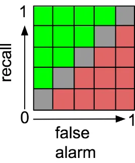
To test this hypothesis, we proposeDODGE(ε), a very fast self-tuning optimization tool. The objective space of the learners (two-dimensional grids of, say, recall vs false alarms) can be divided into cells (“chunks”) of sizeεwhere 1 decision option is harder to distinguish result from another decision option.DODGE(ε)(a) negatively weigh regions of the decision space that fall withinεof old objective space; and (b) selects next samples from regions with least negative weights.
When tested on a variety of case studies from software analytics,DODGE(ε)generates optimiza-tions better than the state of the art in HPO in software analytics tasks such as 1) Defect prediction; 2) SE text mining classification; 3) Bad Code Smell; and 4)Issue Close Time. More importantly, it does so after very few samples (fewer than50) than other state-of-the-art methods.
Performance was scored usingp=2 metrics: 1) for all 4 tasks:recallvsfalse alarmstrade-offs; 2) for defect prediction: howfewmodules must be inspected to findmostbugs. In the comparison, DODGE(.2)produced best performance scores. Further,DODGE(.2)terminated after far fewer evaluations than standard HPO. We conjecture this is becauseDODGE(.2)explores a very small space of 1/εpcells while standard optimizers struggle to cover billions of decision options (most of which yield indistinguishable results).
© Copyright 2019 by Amritanshu Agrawal
On the Nature of Software Engineering Data (Implications ofε-Dominance in Software Engineering)
by
Amritanshu Agrawal
A dissertation submitted to the Graduate Faculty of North Carolina State University
in partial fulfillment of the requirements for the Degree of
Doctor of Philosophy
Computer Science
Raleigh, North Carolina
2019
APPROVED BY:
Dr. Matthias Stallmann Dr. Min Chi
Dr. Jamie Jennings Dr Timothy Menzies
BIOGRAPHY
Amritanshu Agrawal was born in Patna, Bihar, India. He grew up there and completed his high school from Kota, Rajasthan, India.
He attended PES University from 2011 to 2015 and graduated with a B.E in Computer Science Engineering. While at PES, he performed many research projects which resulted in a research publication. He also carried out research in Computer Vision at Durham University, UK under the supervision of Dr Toby Breckon.
ACKNOWLEDGEMENTS
Firstly, I would like to express my sincere gratitude to my advisor Dr Tim Menzies for the continuous support of my Ph.D study and related research, for his patience, motivation, and immense knowledge. His guidance helped me in all the time of research and writing of this thesis. I could not have imagined having a better advisor and mentor for my Ph.D study.
Besides my advisor, I would like to thank the rest of my thesis committee: Dr Matthias Stallmann, Dr Min Chi, and Dr. Jamie Jennings, for their insightful comments and encouragement, but also for the hard question which incented me to widen my research from various perspectives.
I thank my fellow labmates in for the stimulating discussions, for the sleepless nights we were working together before deadlines, and for all the fun we have had in the last four years.
TABLE OF CONTENTS
LIST OF TABLES . . . vi
LIST OF FIGURES. . . vii
Chapter 1 INTRODUCTION . . . 1
1.1 Contribution . . . 5
1.2 External Validity and Future work . . . 7
1.3 Statement of Thesis . . . 7
1.4 Research Articles . . . 7
1.4.1 Accepted Papers from this thesis . . . 7
1.4.2 Other PhD papers not part of this thesis . . . 8
1.4.3 Papers Under Review part of this thesis . . . 8
1.5 Structure of this Thesis . . . 8
Chapter 2 Background and Motivation . . . 10
2.1 Hyperparameter Tuning . . . 10
2.1.1 Why Explore Faster Software Analytics? . . . 11
2.2 Background . . . 14
2.2.1 SE: Defect Prediction . . . 14
2.2.2 SE: Text Mining . . . 17
2.2.3 SE: Bad Code Smell Detection . . . 20
2.2.4 SE: Issue Lifetime Estimation . . . 21
2.2.5 NON-SE: UCI Repository . . . 22
2.3 Existence and Exploitation ofε. . . 23
2.4 Summary . . . 24
Chapter 3 Discussion of the Methodology . . . 26
3.1 Datasets . . . 27
3.1.1 Defect Prediction . . . 27
3.1.2 Text Mining . . . 30
3.1.3 Bad Code Smell Detection . . . 31
3.1.4 Issue Lifetime Estimation . . . 33
3.1.5 NON-SE: UCI Datasets . . . 34
3.2 Evaluation Criteria . . . 39
3.3 Frameworks . . . 41
3.3.1 Traditional Machine Learning without hyperparameter optimization . . . 41
3.3.2 SMOTE . . . 41
3.3.3 LDA . . . 43
3.3.4 DE . . . 45
3.3.5 SMOTUNED . . . 47
3.3.6 LDADE . . . 47
3.3.7 LDA-GA . . . 48
3.3.9 FLASH . . . 51
3.3.10 DODGE(ε) . . . 52
3.4 Summary . . . 58
Chapter 4 Research Findings . . . 59
4.1 RQ1 . . . 60
4.2 RQ2 . . . 63
4.3 RQ3 . . . 64
4.4 RQ4 . . . 66
4.5 RQ5 . . . 68
4.6 RQ6 . . . 75
4.7 Discussion on Results . . . 81
Chapter 5 Threats to Validity . . . 85
5.1 Sampling Bias . . . 85
5.2 Learner Bias . . . 85
5.3 Evaluation Bias . . . 86
5.4 Order Bias . . . 86
5.5 Construct Validity . . . 86
5.6 Statistical Validity . . . 86
5.7 External Validity . . . 86
Chapter 6 Conclusion. . . 88
6.1 Limitations of Current Methodologies . . . 89
6.2 Future Work . . . 89
LIST OF TABLES
Table 2.1 Notes on different optimizers used in our case study . . . 12
Table 2.2 22 highly cited Software Defect prediction studies. . . 15
Table 2.3 Top SE venues that published on Text Mining using Topic Modeling from 2009 to 2016. . . 18
Table 2.4 Literature Review of Text Mining Papers in SE. . . 19
Table 3.1 Frameworks comparison used with different SE and NON-SE tasks . . . 27
Table 3.2 Attributes in Defect Prediction Data . . . 28
Table 3.3 Defect Prediction Open-Source Java Systems . . . 29
Table 3.4 SMOTE parameters . . . 29
Table 3.5 Classifiers used by SMOTUNED . . . 30
Table 3.6 Text Mining Dataset . . . 31
Table 3.7 Bad Code Smell Detection Dataset . . . 32
Table 3.8 Static code metrics used in code smells data sets. . . 33
Table 3.9 Issue Lifetime Estimation Dataset . . . 35
Table 3.10 Issue Lifetime Estimation Dataset Continued . . . 36
Table 3.11 Metrics used in Issue lifetime data . . . 37
Table 3.12 NON-SE: 37 UCI Datasets . . . 38
Table 3.13 Traditional Machine Learning Algorithms . . . 42
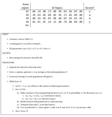
Table 3.14 Example of Topics generated By LDA . . . 45
Table 3.15 Document Topic distribution found by LDA for PitsA dataset . . . 46
Table 3.16 List of LDA parameters tuned by DE . . . 48
Table 3.17 Lower and Upper Bound Samples Needed. . . 53
Table 3.18 Hyperparameter Tuning Options Explored for Data Preprocessing . . . 56
Table 3.19 Hyperparameter Tuning Options Explored for Learners . . . 57
Table 4.1 RQ5: Summarized Issue Lifetime Prediction results comparison against all frameworks . . . 75
LIST OF FIGURES
Figure 1.1 Grids in results space. . . 3
Figure 1.2 Evaluations taken by different Frameworks for Text Mining . . . 5
Figure 2.1 Data Growth 2005-2015, from[NY14]. . . 17
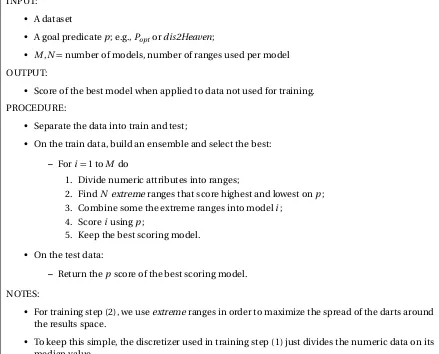
Figure 3.1 Effort-based cumulative lift chart[Yan16]. . . 40
Figure 3.2 Pseudocode of SMOTE . . . 43
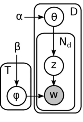
Figure 3.3 LDA . . . 44
Figure 3.4 Differential Evolution . . . 46
Figure 3.5 FFT: an ensemble algorithm to sample results space,M number of times. . . . 49
Figure 3.6 A simple model for software defect prediction . . . 50
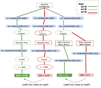
Figure 3.7 An example ofDODGE(.05)tree structure . . . 55
Figure 4.1 DODGE(ε)finds optimal performance very quickly. . . 60
Figure 4.2 Defect Prediction results for constantN and varyingε . . . 61
Figure 4.3 Defect Prediction results for constantN and varyingε . . . 62
Figure 4.4 Text Mining results for constantN and varyingεas well as varyingN and constantε . . . 62
Figure 4.5 RQ2: Defect Prediction comparison against all the frameworks . . . 64
Figure 4.6 RQ2: Defect Prediction results comparison ofDODGE(.2)against FLASH . . . 65
Figure 4.7 RQ3: Text Mining results comparison against all frameworks . . . 66
Figure 4.8 RQ4: Bad Smell results comparison against all frameworks . . . 67
Figure 4.9 RQ5: 1 Day, Issue Lifetime Prediction results comparison against all frameworks 68 Figure 4.10 RQ5: 7 Days, Issue Lifetime Prediction results comparison against all frameworks 69 Figure 4.11 RQ5: 14 Days, Issue Lifetime Prediction results comparison against all frame-works . . . 70
Figure 4.12 RQ5: 30 Days, Issue Lifetime Prediction results comparison against all frame-works . . . 71
Figure 4.13 RQ5: 90 Days, Issue Lifetime Prediction results comparison against all frame-works . . . 72
Figure 4.14 RQ5: 180 Days, Issue Lifetime Prediction results comparison against all frame-works . . . 73
Figure 4.15 RQ5: 365 Days, Issue Lifetime Prediction results comparison against all frame-works . . . 74
Figure 4.16 RQ6: UCI Datasets comparison against all frameworks . . . 76
Figure 4.17 RQ6: UCI Datasets-continued comparison against all frameworks . . . 77
Figure 4.18 RQ6: UCI Datasets-continued comparison against all frameworks . . . 78
CHAPTER
1
INTRODUCTION
This thesis argues on the nature of Software engineering data and how is it different than other domains. We believeSoftware analytics can be inherently simplewhich means that much prior research [Fu16a; Men07a; AM18]hasneedlessly complicated an inherently simple task. Here by “simple” we mean that very little CPU is required to build software quality prediction models. We
show that this is true for four SE tasks:
• Software defect prediction; i.e. the classification of software modules into “buggy” or otherwise based on static code attributes[Fu16a; Tan16; Men07a; AM18];
• Software bug report text mining; i.e. text mining algorithms that rank or predict issue reports severity[Agr18b; Oli10a];
• Detecting bad code smells; i.e., the prediction of defect modules due to the presence of bad code smells[KM18];
• Issue lifetime estimation; i.e., predicting the time it takes to close an issue[Che18; KM18].
Fu16a; Agr18b; TW18; Liu10; Sar12; Tan16; Zho04; Oli10a]. The problem with HPO is that tuning requires high number of evaluations to test hundreds to millions of different tuning options and the cost of running a data miner through all those options is very high, requiring days to weeks to decades of CPU[Wan13; TW18].
For many years, we have addressed these long CPU times via cloud-based CPU farms. For example, many of the experiments conducted in software analytics can be easily parallelized just by running (e.g.) multiple sub-samples of the data on separate cores. But that process can be very expensive. Fisher et al.[Fis12]comment that cloud computation is a heavily monetized environment that charges for all their services (storage, uploads, downloads, and CPU time). While each small part of that service is cheap, the total annual cost to an organization can be exorbitant.
Though, recently we developed faster HPO methods like SMOTUNED for defect prediction task and LDADE for SE text mining task which took 50 and 30 evaluations respectively to achieve better performance than other HPOs for similar tasks. More recently we developed FFtrees[Phi17; Che18; Fu18], and surprisingly, FFtrees (a) save most of CPU cost while at the same time (b) find better tunings. FFtrees out-perform many of state-of-the-art SE HPOs, and our own developed LDADE and SMOTUNED, for different SE tasks understudy. This was a very strange observation since tuning sampled hundreds to thousands of options, while FFtrees explored only 16.
These few examples motivated us further to conjecture that
1. Something might be grouping the output space into “chunks” such that
2. looking at a few samples is just as effective as looking at many more.
To explain what causes that grouping, we note that analytics is a probabilistic process where different treatments produce different distributions of results. When comparing distributions to show that, say, tuning1 is better than tuning2, there is always some deltaεin the results below which it is hard to distinguish different treatments. As shown in Figure 1.1,εdivides the output space of a learner into 1/εp cells, wherep is the number of performance scores being monitored. Forp=2, andε=0.2, that output space divides into just 25 cells (where green is preferred over red).
Figure 1.1Grids in results space.
• For all four SE tasks:recallvsfalse alarmstrade-offs.
• For defect prediction: howfewmodules must be inspected to findmostbugs.
To certify the value of this approach, this thesis explores 3 research questions:
• RQ1: IsDODGE(ε)too complicated? Is it difficult to determine its{N,ε}values?
This thesis propose simplifications to software analytics (where lesser evaluations define simplicity), it is important to check if the new proposed method is itself simple to apply. Accordingly, this research question asks if it is difficult to find useful values for N (the number of evaluations) or theε value (“chunk” size) used in the search.
• RQ2: How doesDODGE(ε)compare to recent prominent defect prediction and hyperparamter optimization results?
Defect prediction is studied extensively among SE researchers using many complex methods, it is important to validate howDODGE(ε)performs to those methods.
• RQ3: How doesDODGE(ε)compare to recent prominent text mining and hyperparamter optimization results?
To show how prominentDODGE(ε)is for the SE tasks, we explored text mining as well. Text mining has become another interesting direction for researchers due to the complexity of the data in use.
DODGE(ε)was also applied to detect defective modules due to the presence of bad code smells.
• RQ5: How doesDODGE(ε)compare to recent prominent issue lifetime prediction and hyper-paramter optimization results?
We also usedDODGE(ε)to predict different issues lifetime (1 day, 7 days, 14 days, 30 days, 90 days, 180 days, 365 days).
• RQ6: What inference can be drawn about SE data compared against other domain data (UCI datasets) after applyingDODGE(ε)?
We also appliedDODGE(ε)to non-SE domain where the data came from popular UCI reposi-tory[AN07; DG17]. We wanted to see whether our hypothesis of objective space being grouped into “chunks” hold true for non-SE domain or not. If not, then how is the data different between the SE
and non-SE domain?
We found thatε=0.2 which comes under largeεvariabilities of SE data, making SE data more peculiar and different.DODGE(.2)produced best performance scores than FFtrees, SMOTUNED, LDADE, FLASH[Nai18]and other state-of-the-art HPOs. Further,DODGE(.2)terminated after far fewer evaluations than standard optimizers. Figure 1.2 represents number of evaluations taken by different frameworks and HPOs for SE tasks.DODGE(ε)explores billions of choices through preprocessors, and machine learners, while performing the best in only 30 evaluations. FFtree builds 16 trees but only explores few ranges. SMOTUNED takes about 50 evaluations to tune only few choices of SMOTE. On another hand, LDADE and LDA-GA takes 300 and 1000 to 10,000 evaluations respectively, to tune only the choices of LDA and performing worse thanDODGE(ε).DODGE(ε) explore billions of choices, the most among other frameworks, while performing the best with just 30 evaluations. We conjecture this is becauseDODGE(.2)explores a very small space of 1/εp cells while standard optimizers struggle to cover billions of tuning options (most of which yield indistinguishably different results).
Figure 1.2Evaluations taken by different Frameworks for Text Mining
The rest of this thesis discusses the why and how of software analytics simplification and the existence ofε-domination in SE data giving the simplified nature of SE data. When we say SE data is different innature, we say that there existsεor have “chunks” where redundant options lead to indistinguisable results. It was also argued that doesεsize “chunks” exists in non-SE domain as well or not. We appliedDODGE(.2)for UCI datasets which are all non-SE domain and found that we didn’t achieve better performance than the tradition machine learning methods. We tried looking at the feature distribution for both SE and non-SE data, and found thatDODGE(ε)works really well when data is 1) highly imbalanced, and 2) if discretization of features works. Finally, it can be concluded that SE data containsεand not the non-SE data. Also,DODGE(ε)can be applied with highly imbalanced datasets and good discretization methods like Fayyad & Irani’s[FI93].
The next section provide background, and argues that such simplifications is useful. Next, we discuss the design and methodology of some of our faster developed HPOs like LDADE and SMOTUNED, FFtree, FLASH and then the framework ofDODGE(ε). All these frameworks provide better improvement and at the same time reduction in number of evaluations as we study them. After that, we reports experiments that compareDODGE(ε)to prior state-of-the-art results. Our conclusion will be thatDODGE(ε)is much better, at reducing the number of evaluations required to find good tunings for software analytics.
1.1
Contribution
commonly contains “chunks” of sizeε. Also,DODGE(ε)defects our all the recently newly created frameworks (our past 3 years of work), namely:
• SMOTUNED[AM18]which was faster and better than all the previous state-of-the-art methods in defect prediction beforeDODGE(ε).
• LDADE[Agr18b]which was faster and better than all the previous state-of-the-art methods in text mining beforeDODGE(ε).
• FFtree[Agr18a; Che18]which was faster and better than all the previous state-of-the-art methods in both defect prediction and text mining beforeDODGE(ε).
• Explored 2 more tasks such as Bad code smell detection, and issue lifetime estimation to compareDODGE(ε)against previous state-of-the-art methods.
But we would also like to propose a new characterization of software analytics:
Software analytics is that branch of machine learning that studies problems with large amounts of variabilityεin their nature.
(For reasons why SE has such largeεvariability , see 2.3.)
This new characterization is a significant contribution since it means that every new machine learning algorithm developed in the AI community might not apply to SE as proved by applying DODGE(ε)on non-SE data. Perhaps understanding SE is a different problem to understanding other problems that are more precisely controlled and restrained. Also, perhaps, it is time to design new machine learning algorithms (likeDODGE(ε)) that are better suited to the largeεvariabilities of SE data. As shown in this thesis, such new algorithms can exploit the peculiarities of SE data to dramatically simplify software analytics.
At last, we have open sourced all the data and code scripts for other students/researchers to refute and reproduce results. Our work is distributed across multiple repositories which are:
• https://github.com/ai-se/e-dom contains our code and data which was used forDODGE(ε) framework.
• https://github.com/ai-se/Smote_tune contains our code and data which was used for SMO-TUNED framework.
• https://github.com/amritbhanu/LDADE-package contains only our reproduction package for LDADE.
1.2
External Validity and Future work
This thesis’s results are based on an analysis of 4 SE tasks and many non-SE tasks which begs the question: how many other domains can be simplified in a similar manner?.
Though it will be needed to explore more tasks with different problems like regression before the methods of this paper can be broadly applied. This would be a fruitful direction for future work.
1.3
Statement of Thesis
Software Engineering is muchsimplerwhen measured in terms of CPU, than other Machine Learn-ing tasks since SE data often conforms toε-dominationwhich can be exploited to produce better learners. Due to the existence ofε-domination, we can avoid spending time, effort and resources on trying billions of ways to tune learners to produce optimal performance.
1.4
Research Articles
1.4.1 Accepted Papers from this thesis
• Amritanshu Agrawal, Wei Fu, Di Chen, Xipeng Shen and Tim Menzies. “Can weDODGE(ε) Complex Software Analytics?”. IEEE Transactions on Software Engineering (2019).
• Amritanshu Agrawal, Wei Fu, and Tim Menzies. “What is wrong with topic modeling? And how to fix it using search-based software engineering.” Information and Software Technology (2018). It contributed to the case study on LDADE for text mining as a motivation for this thesis.
• Amritanshu Agrawal, and Tim Menzies. “Is better data better than better data miners?: on the benefits of tuning SMOTE for defect prediction.” International Conference on Software Engineering (2018). It contributed to the case study on SMOTUNED for Defect Prediction as a motivation for this thesis.
• George Mathew,Amritanshu Agrawal, and Tim Menzies. “Finding Trends in Software Re-search.” IEEE Transactions on Software Engineering (2018). It showed LDADE to improve topic stability in bibliometric SE text mining study.
• George Mathew,Amritanshu Agrawal, and Tim Menzies. “Trends in topics at SE conferences (1993-2013)” ICSE-C (2016). It showed LDADE to improve topic stability in bibliometric SE text mining study.
1.4.2 Other PhD papers not part of this thesis
• Amritanshu Agrawal, Akond Rahman, Rahul Krishna, Alexander Sobran, and Tim Menzies. “We don’t need another hero?: the impact of heroes on software development.” International
Conference on Software Engineering: Software Engineering in Practice (2018).
• Rahul Krishna,Amritanshu Agrawal, Akond Rahman, Alexander Sobran, and Tim Menzies. “What is the connection between issues, bugs, and enhancements?: lessons learned from 800+ software projects.” International Conference on Software Engineering: Software Engineering in Practice (2018).
• Akond Rahman,Amritanshu Agrawal, Rahul Krishna, and Alexander Sobran. “Characterizing The Influence of Continuous Integration: Empirical Results from 250+Open Source and Proprietary Projects.” Swan Workshop, FSE 2018
• Rahul Krishna, Zhe Yu,Amritanshu Agrawal, et al. “The ’BigSE’ Project: Lessons Learned from Validating Industrial Text Mining” BIGDSE Workshop, ICSE 2016.
• Suvodeep Majumder, Joymallya Chakraborty,Amritanshu Agrawal, and Tim Menzies. “Why Software Projects need Heroes (Lessons Learned from 1100+Projects)” Under Review, IEEE Transactions on Software Engineering 2019.
1.4.3 Papers Under Review part of this thesis
• Amritanshu Agrawaland Tim Menzies. “DODGE(ε)works for Bad Code Smell and Issue Lifetime Prediction”.
• Amritanshu Agrawal, Huy Tu and Tim Menzies. “Can You Explain That, Better? Comprehen-sible Text Analytics for SE Applications”.
1.5
Structure of this Thesis
The rest of this report is structured as follows:
• Chapter 2 gives a brief background about optimizers and different SE tasks studied in this thesis. It also provides the motivation for the existence ofε.
• Chapter 4 talks about results and answers to 6 research questions.
• Chapter 5 discusses about threats to validity of this study.
CHAPTER
2
BACKGROUND AND MOTIVATION
In this chapter we will give a brief background about hyperparameter tuning and literature review on different optimizers and what optimizers did we select for our study and why. It will be followed up with the discussion on defect prediction, text mining, bad code smell detection and issue lifetime estimation SE tasks, and why did we study these SE tasks, its related past work. We will also talk about why we chose UCI datasets as the source for non-SE domain. We will explain how did we come up with our hypothesis of largeεor existence ofε-domination in the nature of SE data.
2.1
Hyperparameter Tuning
Hyperparameter tuning is a subset to an optimization problem. Data mining is a problem that involves finding an approximation ˆh(x)of a function of the following format:
y=h(x) (2.1)
wherex= (x1,···,xp)∈Xare the input variables,y= (y1,···,yq)∈Yare the output variables of the functionh(x):X→Y,Xis the input space andY is the output space. The input variablesxare frequently referred to as the independent variables or input features, whereasyare referred to as the dependent variables or output features.
could be a label identifying the component as defective or non-defective. Many different machine learning algorithms can be used for data mining.
The functionsh(x)and ˆh(x)maynot necessarily correspond to the optimization functions. However, the true functionh(x)is unknown. Therefore, data mining frequently relies on machine learning algorithms to learn an approximation ˆh(x)based on a setD={(xi,yi)}|iD=1| of known examples (data points) fromh(x). And, learning this approximation typically consists of searching for a function
ˆ
h(x)that minimizes the error (or other predictive performance metrics) on examples fromD. These machine learning algorithms also come up with their own parameters which can give rise to different approximations while learning about the data. Hyperparameter tuning is an art of tuning the parameters that control the choices within a data miner. They also try to minimizes or maximizes the performance metric. In our case, we used a multi-goal optimization problem where we either minimized or maximized the goals for our 4 SE tasks understudy.
The impact of hyperparameter tuning is well understood in the theoretical machine learning literature[BB12]. When we tune a data miner, what we are really doing is changing how a learner applies its heuristics. This means tuned data miners use different heuristics, which means they ignore different possible models, which means they return different models, i.e.,howwe learn changeswhatwe learn.
Tuning has been addressed in many software analytics literature. Fu et al.[Fu16a]surveyed hundreds of recent SE papers in the area of software defect prediction from static code attributes. Tantithamthavorn et al.[Tan16]explored tunings for many learners. In general, the importance of tuning is extensively mentioned.
Bergstra et al.[BB12]commented thatgrid search1is very popular since (a) such a simple search to gives researchers some degree of insight; (b) grid search has very little technical overhead for its implementation; (c) it is simple to automate and parallelize; (d) on a computing cluster, it can find better tunings than sequential optimization (in the same amount of time). That said, grid search is not efficient due to extensive options that it explores.
The literature mentions many faster optimizers than grid search like simulated annealing[FM02; Men07c]; various genetic algorithms[Gol79]augmented by techniques such as DE (differential evolution[SP97]), tabu search and scatter search[GM86; Bea06; Mol07; Neb08]; particle swarm optimization[Pan08]; numerous decomposition approaches that use heuristics to decompose the total space into small problems, then apply a response surface methods[Kra15; Zul13]. Table 2.1 shows the optimizers that were used in this thesis.
2.1.1 Why Explore Faster Software Analytics?
This section argues that avoiding slow methods for software analytics is an open and urgent issue.
Table 2.1Notes on different optimizers used in our case study
Genetic Algorithms (GAs)execute over multiple generations. Generation zero is usually initialized at random. After that, in each generation, candidate items are subject to select (prune away the less interesting solutions), crossover (build new items by combining parts of selected items), and mutate (randomly perturb part of the the new solutions). Modern GAs take different approaches to the select operator (see https://raw.githubusercontent.com/txt/ase16/master/img/rankvscountvsdepth.png). Notable exceptions are MOEA/D that use a decomposition operator to divide all the solutions into many small neighborhoods where if anyone finds a better solution, all its neighbors move there as well[AC05; HC06; CH07; Sar16; Oli10a; Pan13; Du15; MY13; Sar12].
Different evolution (DE)execute over multiple generations. Generation zero is usually initialized at random. After that, in each generation, candidate items are subject toselect
(prune away the less interesting solutions),mutate(build new items by combining with 3 other random candidates from the same generation)[SP97; Fu16a; AM18; Agr18b; FM17; Men18].
Researchers and industrial practitioners now routinely make extensive use of software analytics to discover (e.g.) how long it will take to integrate the new code[Cze11], where bugs are most likely to occur[Ost04], who should fix the bug[Anv06], or how long it will take to develop their code[Koc12b; Koc12a; MJ03]. Large organizations like Microsoft routinely practice data-driven policy development where organizational policies are learned from an extensive analysis of large data sets collected from developers[BZ14; The15].
But the more complex the method, the harder it is to apply the analysis. Fisher et al.[Fis12] characterizes software analytics as a work flow that distills large quantities of low-value data down to smaller sets of higher value data. Due to the complexities and computational cost of SE analyt-ics, “the luxuries of interactivity, direct manipulation, and fast system response are gone”[Fis12]. They characterize modern cloud-based analytics as a throwback to the 1960s-batch processing mainframes where jobs are submitted and then analysts wait, wait, and wait for results with “little insight into what is really going on behind the scenes, how long it will take, or how much it is going to cost”[Fis12]. Fisher et al. [Fis12]document the issues seen by 16 industrial data scientists, one of whom remarks
“Fast iteration is key, but incompatible with the jobs are submitted and processed in the cloud. It is frustrating to wait for hours, only to realize you need a slight tweak to your feature set”.
Methods for improving the quality of modern software analytics have made this issue even more serious. There has been continuous development of new feature selection[HH03]and feature discovering[Jia13]techniques for software analytics, with the most recent ones focused on deep learning methods. These are all exciting innovations with the potential to dramatically improve the quality of our software analytics tools. Yet these are all CPU/GPU-intensive methods. For instance:
• Learning control settings for learners can take days to weeks to years of CPU time[Fu16b; Tan16; Wan13].
• Lam et al. needed weeks of CPU time to combine deep learning and text mining to localize buggy files from bug reports[Lam15].
• Gu et al. spent 240 hours of GPU time to train a deep learning based method to generate API usage sequences for given natural language query[Gu16].
of CPU time to learn the tuning parameters of software clone detectors proposed in [Wan13]. Much of that CPU time can be saved if there is a faster way.
2.2
Background
This section we will provide background on each case study for this thesis, which are: defect predic-tion, text mining, bad code smell detection and issue lifetime estimation as well as non-SE tasks. This section justifies why these are worthy of inspection and what have been done in the past.
2.2.1 SE: Defect Prediction
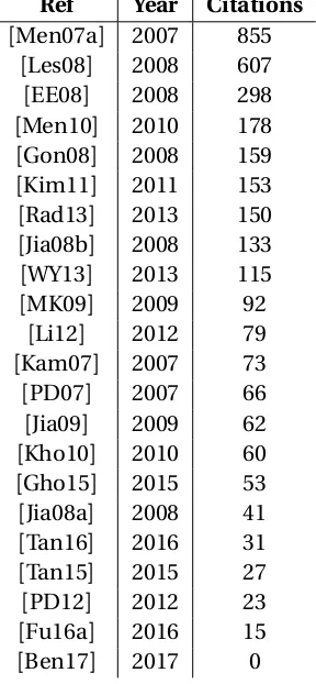
This section argues that defect prediction is a useful area of research, worthy of exploration and simplification. Defect prediction has been more than a decade long study and researchers have come up with different methods, to improve performances in which some are heavy CPU intensive methods like [Tan16]and some are simple. Table 2.2 gives top 22 highly cited Software defect prediction studies done since as early as 2007. This shows that the field of Software defect prediction is largely studied.
A variety of approaches have been proposed to recognize defect-prone software components using code metrics (lines of code, complexity)[D’A10; Men07a; Nag06; She14; Men10]or process metrics (number of changes, recent activity)[Has09]. Other work, such as that of Bird et al.[Bir09], indicated that it is possible to predict which components (for e.g., modules) are likely locations of defect occurrence using a component’s development history and dependency structure. Prediction models based on the topological properties of components within them have also proven to be accurate[ZN08].
The lesson of all the above is that the probable location of future defects can be guessed using logs of past defects[Hal12; CD09]. These logs might summarize software components using static code metrics such as McCabes cyclomatic complexity, Briands coupling metrics, dependencies between binaries, or the CK metrics[CK94]. One advantage with CK metrics is that they are simple to compute and hence, they are widely used. Radjenovi´c et al.[Rad13]reported that in the static code defect prediction, the CK metrics are used twice as much (49%) as more traditional source code metrics such as McCabes (27%) or process metrics (24%). Note that such attributes can be automatically collected, even for very large systems[NB05]. Other methods, like manual code reviews, are far slower and far more labor intensive.
Table 2.222 highly cited Software Defect prediction studies. Defect prediction is largely studied field.
Ref Year Citations
[Men07a] 2007 855 [Les08] 2008 607 [EE08] 2008 298 [Men10] 2010 178 [Gon08] 2008 159 [Kim11] 2011 153 [Rad13] 2013 150 [Jia08b] 2008 133
[WY13] 2013 115
[MK09] 2009 92 [Li12] 2012 79
[Kam07] 2007 73
[PD07] 2007 66 [Jia09] 2009 62
[Kho10] 2010 60
[Gho15] 2015 53 [Jia08a] 2008 41 [Tan16] 2016 31 [Tan15] 2015 27 [PD12] 2012 23 [Fu16a] 2016 15
[Ben17] 2017 0
Jlint, and (b) static code defect predictors. This is an interesting result since it is much slower to adapt static code analyzers to new languages than defect predictors (since the latter just requires hacking together some new static code metrics extractors).
Software developers are smart, but sometimes make mistakes. In a survey done by NIST in 2002, it was found that software defects and failures can cost upto $60 billion a year in the US itself.[Tas02]. Hence, it is essential to test software before the deployment [OR14; Bar15; YH12; Mye11]. Software quality assurance budgets are finite while assessment effectiveness increases exponentially with assessment effort[Fu16a]. Therefore, standard practice is to apply the best available methods on code sections that seem most critical and bug-prone. Software bugs are not evenly distributed across the project[HGP09; Kor09; Ost04; Mis11]. Hence, a useful way to perform software testing is to allocate most assessment budgets to the more defect-prone parts in software projects. Software defect predictors are never 100% correct. But they can be used to suggest where to focus more expensive methods.
that over 90% of the respondents were willing to adopt defect prediction techniques. Other results from commercial deployments show the benefits of defect prediction. When Misirli et al. [Mis11] built a defect prediction model for a telecommunications company, those models could predict 87 percent of code defects. Those models also decreased inspection efforts by 72 percent, and hence reduce post-release defects by 44 percent. Also, when Kim et al.[Kim15]applied defect prediction model, REMI, to API development process at Samsung Electronics, they found they could predicted the bug-prone APIs with reasonable accuracy (0.68 F1 score) and reduced the resources required for executing test cases.
Software defect predictors not only save labor compared with traditional manual methods, but they are also competitive with certain automatic methods. Given this equivalence, it is significant to note that static code defect prediction can be quickly adapted to new languages by building lightweight parsers to extract static code metrics such as CK metrics[CK94]. The same is not true for static code analyzers - these need extensive modification before they can be used in new languages.
Class imbalance is concerned with the situation in where some classes of data are highly under-represented compared to other classes[HG09]. By convention, the under-represented class is called theminorityclass, and correspondingly the class which is over-represented is called themajority
class. In this paper, we say that class imbalance isworsewhen the ratio of minority class to majority
increases, that is,class-imbalance of 5:95is worse than20:80. Menzies et al.[Men07b]reported SE data sets often contain class imbalance. In their examples, they showed static code defect prediction data sets with class imbalances of 1:7; 1:9; 1:10; 1:13; 1:16; 1:249.
Figure 2.1Data Growth 2005-2015, from[NY14].
2.2.2 SE: Text Mining
The current great challenge in software analytics is understanding unstructured data. As shown in Figure 2.1, most of the planet’s 1600 Exabytes of data does not appear in structured sources (databases, etc)[NY14]. Mostly the data is ofunstructuredform, often in free text, and found in word processing files, slide presentations, comments, etc. Such unstructured data does not have a pre-defined data model and is typically text-heavy. Finding insights among unstructured text is difficult unless we can search, characterize, and classify the textual data in a meaningful way.
The earliest results from software analytics come from relatively simpler problems (e.g. defect prediction applied to structured data). To some extent, this was due to relative simplicity of the problem. In defect prediction, a single example is some unit of code such as module or function or class. Since that code can compile, then by definition, that unit of code has a precisely defined syntax and semantics. In practice, such code modules are described in just a few dozen attributes. Lately, there has been much more interest in SE text mining[Men08a; MM08; Pan13; Agr18b; Xu16; Men18]since this covers a much wider range of SE activities. Text mining is a harder problem than defect prediction. Free form natural language is semantically very complex and may not conform to any known grammar. In practice, such text documents may be described using tens of thousands of attributes (one for each word in the natural language of the author of those documents). For example, consider NASA’s software project and issue tracking systems (or PITS)[Men08a; MM08]. PITS contains text that discusses bugs and changes in source code. It also contains and comments on software patches.
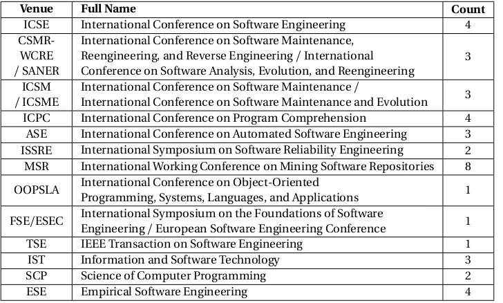
Table 2.3Top SE venues that published on Text Mining using Topic Modeling from 2009 to 2016.
Venue Full Name Count
ICSE International Conference on Software Engineering 4
CSMR-WCRE
/SANER
International Conference on Software Maintenance, Reengineering, and Reverse Engineering/International Conference on Software Analysis, Evolution, and Reengineering
3 ICSM
/ICSME
International Conference on Software Maintenance/
International Conference on Software Maintenance and Evolution 3 ICPC International Conference on Program Comprehension 4 ASE International Conference on Automated Software Engineering 3 ISSRE International Symposium on Software Reliability Engineering 2 MSR International Working Conference on Mining Software Repositories 8 OOPSLA International Conference on Object-Oriented
Programming, Systems, Languages, and Applications 1 FSE/ESEC International Symposium on the Foundations of Software
Engineering/European Software Engineering Conference 1 TSE IEEE Transaction on Software Engineering 1 IST Information and Software Technology 3 SCP Science of Computer Programming 2 ESE Empirical Software Engineering 4
in prominent SE venues. Tables 2.3[Sun16]and 2.4 show top SE venues that published SE results and a sample of those papers respectively.
As tohowtext mining have been used, it is important to understand the distinction between supervised and unsupervised data mining algorithms. In the general sense, most data mining is “supervised” when you have data samples associated with labels and then use machine learning tools to make predictions. For example, in the case of[Loh13; Sun15], the authors used LDA as a feature extractor to build feature vectors which, subsequently, were passed to a learner to predict for a target class. Note that such supervised LDA processes can be fully automated and do not require human-in-the-loop insight to generate their final conclusions.
However, in case of, “unsupervised learning”, the final conclusions are generated via a manual analysis and reflection over, e.g., the topics generated by topic modeling. Such cases represent[Bar14; Hin12]who used a manual analysis of the topics generated from some SE tasks textual data by LDA as part of the reasoning within the text of that paper. It is possible to combine manual and automatic methods, please see the “Semi-supervised” paper of Le et al.[Le14].
Table 2.4A sample of the recent literature on using Text Mining in SE. Sorted by number of citations (in column3).
REF Year Citations Venues Tasks/Use cases Unsupervised
or Supervised [RK11] 2011 112 WCRE Bug Localisation Unsupervised
[Oli10b] 2010 108 MSR Traceability Link recovery Unsupervised
[Bar14] 2014 96 ESE Stackoverflow Q&A data analysis Unsupervised
[Pan13] 2013 75 ICSE Finding near-optimal configurations Semi-Supervised
[GCW13] 2013 61 ICSE Software RequirementsAnalysis Unsupervised
[Hin11] 2011 52 MSR Software Artifacts Analysis Unsupervised
[GM14] 2014 44 RE Requirements Engineering Unsupervised
[Tho11] 2011 44 ICSE A review on LDA Mining software repositories using topic models
Unsupervised
[Tho14b] 2014 35 SCP Software Artifacts Analysis Unsupervised
[Che12] 2012 35 MSR Software Defects Prediction Unsupervised
[Tho14a] 2014 31 ESE Software Testing Unsupervised
[BL09] 2009 29 MSR Software History Comprehension Unsupervised
[Loh13] 2013 27 ESEC/FSE Traceability Link recovery Supervised
[Bin14] 2014 20 ICPC Source Code Comprehension Unsupervised
[LV13] 2013 20 MSR Stackoverflow Q&A data analysis Unsupervised
[Kol14] 2014 15 WebSci Social Software Engineering Unsupervised
[Gra13] 2013 13 SCP Source Code Comprehension Unsupervised
[Hin12] 2012 13 ICSM Software Requirements Analysis Unsupervised
[Fu15] 2015 6 IST Software re-factoring Supervised
[GM16] 2016 5 CS Review Bibliometrics and citations analysis Unsupervised
[Le14] 2014 5 ISSRE Bug Localisation Semi-Supervised
[Nik15] 2015 3 JIS Social Software Engineering Unsupervised
[Sun15] 2015 2 IST Software Artifacts Analysis Supervised
2.2.3 SE: Bad Code Smell Detection
According to Fowler[Fow99], bad smells (i.e., code smells) are “a surface indication that usually corresponds to a deeper problem”. Studies suggest a relationship between code smells and poor maintainability or defect proneness[YM13; YC13; Zaz11]and therefore, smell detection has be-come an established method to discover source code (or design) problems to be removed through refactoring steps, with the aim to improve software quality and maintenance. Research on software refactoring endorses the use of code-smells as a guide for improving the quality of code as a preven-tative maintenance. Consequently, code smells are captured by popular static analysis tools, like PMD2, CheckStyle3, FindBugs4, and SonarQube5.
Now, most detection tools for code smells make use of detection rules based on the computation of a set of metrics, e.g., well-known object-oriented metrics such as naming[Moh10], structural rules[Moh10], or even version history[Pal13]. Though these rule-based approaches rely heavily on human created rules that must be manually specified. For example, DECOR[Moh10]requires that the rules are specified in the form of domain specific language and this specification process must be undertaken by domain experts, engineers or quality experts. Naturally, this rule creation requires effort from these individuals that could be spent in some other tasks. Whether the metrics based ML-approaches require less effort than rule-based approaches is however not clear, and it depends on two factors; (a) how complex rules one needs for the rule based approaches, and (b) how many training samples are needed for the metrics based machine learning approaches. At the moment, we are not aware of any studies comparing the approaches effort-wise. However, what remains a clear benefit for the metrics based ML- approach is the reduction of cognitive load required from the engineers. The rule-based approach requires that the engineers create specific rules of defining each smell. For the machine learning based approached the rule creation is left for the ML-algorithms requiring the engineers only to provide information whether a piece of code has a smell or not. Also, these object-oriented metrics are used to set some thresholds for the detection of a code smell. But these rules lead to far too many false positives making it difficult for practitioners to refactor code[Kri17].
Recently, the research community is changing rapidly in terms of defining novel methodologies that incorporate additional information to detect code-smells. Much progress has been made in towards adopting machine learning tools to classify code smells from examples, easing the build of automatic code smell detectors, and also due to the problems face in manual detection using object-oriented metrics, thereby providing a better-targeted detection. Maiga et al.[Mai12b] intro-duce SVMDetect, an approach to detect anti- patterns or bad code smell, based on support vector
machines (SVM). The subjects of their study are the Blob, Functional Decomposition, Spaghetti Code and Swiss Army Knife antipatterns, extracted from three open-source programs: ArgoUML, Azureus, and Xerces. Maiga et al.[Mai12a]extended the previous paper by introducing SMURF, which takes into account practitioner’s feedback.
Kreimer[Kre05]proposed an adaptive detection to combine known methods for finding design flaws Large Class and Long Method on the basis of metrics. Khomh et al.[Kho09]proposed a Bayesian approach to detect occurrences of the Blob antipattern on open-source programs. Khomh et al.[Kho11]also presented BDTEX, a GQM approach to build Bayesian Belief Networks from the definitions of antipatterns. Yang et al.[Yan12]study the judgment of individual users by applying machine learning algorithms on code clones. These studies were not included in our comparison as the data was not readily available for us to reuse.
More recently, Fontana et al.[Arc16]in their study of several code smells, considered 74 systems for their analysis and validation. They experimented with 16 different machine learning algorithms. They made available their dataset, which we have adapted for our applications in this study. These datasets were generated using the Qualitas Corpus (QC) of systems[Tem10]. The Qualitas corpus is composed of 111 systems written in Java, characterized by different sizes and belonging to different application domains. Fontana et al.[Arc16]selected a subset of 74 systems for their analysis. The authors computed a large set of object-oriented metrics belonging to class, method, package, and project level. A detailed list of metrics and their definitions are available in appendices of[Arc16].
2.2.4 SE: Issue Lifetime Estimation
Open source projects use issue tracking systems to enable effective development and maintenance of their software systems. Typically, issue tracking systems collect information about system failures, feature requests, and system improvements. Based on this information and actual project planing, developers select the issues to be fixed. Predicting the time it may take to close an issue has multiple benefits for the developers, managers, and stakeholders involved in a software project. Predicting issue lifetime helps software developers better prioritize work; helps managers effectively allocate resources and improve consistency of release cycles; and helps project stakeholders understand changes in project timelines and budgets. It is also useful to be able to predict issue lifetime specifi-cally when the issue is created, since it is found earlier that delaying to resolve issues can become harder and costlier[Men17]. An immediate prediction can be used, for example, to auto-categorize the issue or send a notification if it is predicted to be an easy fix.
65by dividing time into 1, 3, 7, 14, 30 days. Zhang et al.[Zha13]developed a comprehensive system to predict lifetime of issues. They used a Markov model with a kNN-based classifier to perform their prediction. More recently, Rees-Jones et al.[Ree17]showed that using Hall’s CFS feature selector and C4.5 decision tree learner a very reliable prediction of issue lifetime could be made.
Bhattacharya and Neamtiu[BN11]studied how existing models “fail to validate on large projects widely used in bug studies”. In a comprehensive study, they find that the predictive power (measured by the coefficient of determinationR2) of existing models is 30-49%. That study found that there is no correlation between bug-fix likelihood, bug-opener reputation, and time required to close the bug for the three datasets used in their study. Guo et al.[Guo10]evaluated the most predictive factors that affect bug fix time for Windows Vista and Windows 7 software bugs. Unlike[BN11], they found that bug-opener reputation affected fix time; an issue with a high-reputation creator was more likely to get fixed. Bugs are also more likely to get fixed if the bug fixer is in the same team as or in geographical proximity of the bug creator. Guo et. al. conclude that the factors most important in bug fix time are social factors such as history of submitting high-quality bug reports and trust between teams interacting over bug reports.
Marks et al.[Mar11]found that time and location of filing the bug report were the most important factors in predicting Mozilla issues, but severity was most important for Eclipse issues. Priority was not found to be an important factor for either Mozilla or Eclipse. Their models produced lower performance metrics (65% misclassification rate) than subsequent work. Kikas et al.[Kik16]built time-dependent models for issue close time prediction using Random Forests with a combination of static code features, and non-code features to predict issue close time with high performance.
2.2.5 NON-SE: UCI Repository
Till this section, we have only been looking at tasks and data related to SE. We also wanted to explore non-SE tasks in which the data came from popular UCI repository[AN07; DG17].
UCI Machine Learning Data Repository was created in 1987 to foster experimental research in machine learning. It contains over 429 databases from a broad range of problem areas including engineering, molecular biology, medicine, finance and politics. The Machine Learning (ML) Repos-itory is commonly used by industrial and academic researchers. It is widely cited in the artificial intelligence literature and the UCI data sets are the most widely used benchmark for empirical evaluation of new and existing learning algorithms. Over 3800 papers available on the web, cite the repository.
2.3
Existence and Exploitation of
ε
AI researchers have repeatedly concluded that a small number ofkeyvariables determine the behavior of the rest of the system.Keyshave been discovered and rediscovered many times and given different names, including feature subset selection[KJ97], narrows[Mic13], master variables[CB94], and back doors[Wil03]. We mention this since the problem of mining data with keys reduces to just the mining the key variables. For many years, we have been believing the Machine learning problems to be complex and due to that new complex methods (which take high CPU resources) have been proposed like deep learning, HPOs and many more taking days, weeks, years of CPU.
For over a decade now, we have been documenting examples were solutions to SE analytics prob-lems were surprisinglysimple(but untilDODGE(ε), we had no explanation for that phenomenon nor a method to exploit that simplicity). For example, when optimizing requirements engineering, we have often found that most requirements are dependent on just a fewkeychoices. We have ex-ploited this effect to simplify reasoning about requirements engineering models[Has05]. In another case, Panichella et al.[Pan13]took 1,000 to 10,000 of key evaluations to tune the parameters of topic modeling where as Agrawal et al.[Agr18b]achieved the same in just 30 key evaluations.
In software effort estimation, COCOMO model takes many attributes to calculate effort but it was found that only few parameters have the most impact on effort[MS12]. For defect prediction, the variance in performance increases (become more unstable) with more number of samples. Also, the performance optimization of a data imbalance technique was achieved in only 50 evalua-tions[AM18].
Above examples show that minimalist, or less have been better. With this, we should expect that the results from software analytics have some large degree of variabilityε. One way to characterize this thesis is to say:
• Stop treating largeεvariability as a problem;
• Instead, treat largeεvariability as a resource that can be used to simplify software analytics.
According to Menzies and Shepperd[MS12], the variability or uncertainity of software quality predictors come from different choices in the training data and many other factors.
Sampling Bias:Any data mining algorithm inputs multiple examples to make its conclusions. The more diverse the input examples, the greater the variance in the conclusions. And software engineering is a very diverse discipline:
• Software is built by people with variable skills.
• That construction process is performed using a wide range of languages and tools.
• Languages, tools & platforms keep changing.
• Within one project, the problems faced and the purpose served by each software module may be very different (e.g., GUI, database, network connections, business logic, etc.).
• Within the career of one developer, the problem domain, goal, and stakeholders of their software can change dramatically from one project to the next.
Pre-processing: Real world data usually requires some clean-up before it can be used effectively by data mining algorithms. There are many ways to transform the data favorably. The numeric data may be discretized into smaller bins. Discretization can greatly affect the results of the learning: since there may be ways to implement discretization[FI93]; Feature selection is sometimes useful to prune uncorrelated features to the target variable[Che05a]. Also, it can be helpful to prune data points that are very noisy or are outliers[Koc10]. Note that the choices made during pre-processing can introduce some variability in the final results.
Stochastic algorithms: Numerous methods in software quality predictors employ stochastic algorithms that use random number generators. For example, the key to scalability is usually (a) build a model on the randomly selected small part of the data then (b) see how well that works over the rest of the data[Scu10]. Also, when evaluating data mining algorithms, it is standard practice to divide the data randomly into several bins as part of a cross-validation experiment[WF02]. For all these stochastic algorithms, the conclusions are adjusted, to some extent, by the random numbers used in the cross-validation experiments.
All the above examples, complex or simple methods which were proposed is to reduce the uncertainties or in other words try to makeε=0 (uncertainty to nil).
Now consider the implications of largeεfor exploring HPO. Recall that such optimizers find a few useful options by exploring a very large number of options. Given a results space like Figure 1.1, many of those options will fall into the same regions. If we mark which options generate results that fall withinεof other results, then we strive to avoid those options in the future, then theoretically we might be able to search across Figure 1.1, very quickly. This largeεvariability is utilized by DODGE(ε), our framework. Next chapters we will describe our methodlogy and framework used in thesis as well as our result findings.
2.4
Summary
showed why it was needed to study non-SE domain using the datasets available in UCI machine learning repository. We also explained what is so different in nature about SE data by showing examples ofε-domination existence, which can already be seen in many research articles, but no one thought about it or took any measures to exploit this existence.
CHAPTER
3
DISCUSSION OF THE METHODOLOGY
Table 3.1Frameworks comparison used with different SE and NON-SE tasks.
Traditional ML SMOTUNED FFTree FLASH LDA-GA LDA DODGE(ε)
Defect Prediction Ø Ø Ø Ø Ø
Text Mining Ø Ø Ø Ø Ø
Code Smell Detection Ø Ø Ø
Predict Issue Lifetime Ø Ø Ø
Non-SE (UCI) Ø Ø Ø
3.1
Datasets
3.1.1 Defect Prediction
Defect prediction can input a range of attributes. For example, table 3.2 and 3.3 describes some data widely used in this area of research. As shown in table 3.3, this data is available for multiple versions of the same software (from http://tiny.cc/seacraft). This is important since, when applying data mining algorithms to build predictive models, one important principle is not to test on the data used in training. There are many ways to design a experiment that satisfies this principle. Some of those methods have limitations; e.g., leave-one-out is too slow for large data sets and cross-validation mixes up older and newer data (such that data from the past may be used to test on future data). In this work, for each project data, we set the latest version of project data as the testing data and all the older data as the training data. For example, we usepoi1.5,poi2.0,poi2.5data for training predictors, and the newer data,poi3.0is left for testing.
Table 3.3 illustrates the variability of SE data. When we compare the % of Defects in the training and test data, we see that the past can be very different to the future. Observe how the median defect percentage in the training data is 29% but in the test data, it is 49% (i.e. nearly doubled). This tells us that software analytics will forever be an imprecise science (and one of the lessons of this paper is that imprecision can be used to simplify complex tasks like hyperparameter optimization).
One issue with some of the data in table 3.3 is imbalanced class frequencies. If the target class is not common (as in camel, ivy, jedit and to a lesser extent velocity and synapse), it can be difficult for a data mining algorithm to generate a model that can locate it. A standard method for addressing class imbalance is the SMOTE pre-processor[Cha02]. SMOTE randomly deletes members of the majority class while synthesizing artificial members of the minority class. SMOTE is controlled by the parameters shown in Table 3.4.
Table 3.2OO CK code metrics used for all studies in this paper. The last line shown, denotes the dependent variable.
amc average method complexity e.g., number of JAVA byte codes
avg, cc average McCabe average McCabe’s cyclomatic complexity seen in class
ca afferent couplings how many other classes use the specific class. cam cohesion amongst classes summation of number of different types of
method parameters in every method divided by a multiplication of number of different method parameter types in whole class and number of methods.
cbm coupling between methods total number of new/redefined methods to which all the inherited methods are coupled cbo coupling between objects increased when the methods of one class access
services of another.
ce efferent couplings how many other classes is used by the specific class.
dam data access ratio of the number of private (protected)
at-tributes to the total number of atat-tributes dit depth of inheritance tree
ic inheritance coupling number of parent classes to which a given class is coupled
lcom lack of cohesion in methods number of pairs of methods that do not share a reference to an case variable.
locm3 another lack of cohesion measure if m,a are the number of
m e t h o d s,a t t r i b u t e s in a class num-ber and µ(a) is the number of methods accessing an attribute, then l c o m3 =
((1 a
P
,jaµ(a,j))−m)/(1−m). loc lines of code
max, cc maximum McCabe maximum McCabe’s cyclomatic complexity
seen in class
mfa functional abstraction no. of methods inherited by a class plus no. of methods accessible by member methods of the class
moa aggregation count of the number of data declarations (class
fields) whose types are user defined classes noc number of children
npm number of public methods
rfc response for a class number of methods invoked in response to a message to the object.
wmc weighted methods per class
defect defect Boolean: where defects found in post-release
Table 3.3Some open-source JAVA systems. Used for training and testing, showing different details for each.
Training Testing
Data Set Versions Cases % Defective Versions Cases % Defective
jedit 3.2, 4.0, 4.1, 4.2 1257 23 4.3 492 2
ivy 1.1, 1.4 352 22 2.0 352 11
camel 1.0, 1.2, 1.4 1819 21 1.6 965 19
synapse 1.0, 1.1 379 20 1.2 256 34
velocity 1.4, 1.5 410 70 1.6 229 34
lucene 2.0, 2.2 442 53 2.4 340 59
poi 1.5, 2, 2.5 936 46 3.0 442 64
xerces 1.0, 1.2, 1.3 1055 16 1.4 588 74
log4j 1.0, 1.1 244 29 1.2 205 92
xalan 2.4, 2.5, 2.6 2411 38 2.7 909 99
Table 3.4SMOTE parameters
Para
Defaults used by SMOTE
Tuning Range (Explored by (SMOTUNED)
Description
k 5 [1,20] Number of neighbors
m 50% {50, 100, 200, 400} Number of synthetic examples to create. Ex-pressed as a percent of final training data.
r 2 [0.1,5] Power parameter for the Minkowski
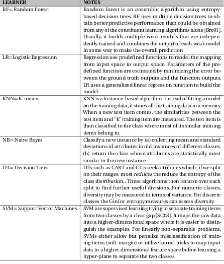
Table 3.5Classifiers used by SMOTUNED. Rankings from Ghotra et al.[Gho15].
RANK LEARNER NOTES
1 “best” RF=random forest Random forest of entropy-based decision trees. LR=Logistic regression A generalized linear regression model.
2 KNN=K-means Classify a new instance by finding “k” examples of similar in-stances. Ghortra et al. suggestedK=8.
NB=Naive Bayes Classify a new instance by (a) collecting mean and standard devia-tions of attributes in old instances of different classes; (b) return the class whose attributes are statistically most similar to the new instance.
3 DT=decision trees Recursively divide data by selecting attribute splits that reduce the entropy of the class distribution.
4 “worst” SVM=support vector machines Map the raw data into a higher-dimensional space where it is easier to distinguish the examples.
from each other). We took couple of learners from each group for the case study of SMOTUNED as shown in table 3.5.
We comparedDODGE(ε)to traditional machine learning algorithms[Gho15], HPO tuning a classifier[Fu16a], HPO tuning a preprocessor[AM18], FFtree[Che18], and FLASH[Nai18]. These all comparisons have shown to work really well in the past.
3.1.2 Text Mining
Table 3.6 describe our PITS data.PITSis a text mining data set generated from NASA software project and issue tracking system (PITS) reports[Men08a; MM08]. This text discusses bugs and changes found in big reports and review patches. Such issues are used to manage quality assurance, to support communication between developers. Topic modeling in PITS can be used to identify the top topics which can identify each severity separately. The dataset can be downloaded from the PROMISE repository[Men15]. Note that, this data comes from six different NASA projects, which we label as PitsA, PitsB, etc.
For this study, all datasets were preprocessed using the usual text mining filters[Fel06]. We implemented stop words removal using NLTK toolkit1[Bir06](to ignore very common short words such as “and” or “the”). Next, Porter’s stemming filter[Por80]was used to delete uninformative word endings (e.g., after performing stemming, all the following words would be rewritten to “connect”: “connection”, “connections”, “connective”, “connected”, “connecting”).
Tf-idf word reduction: focus on the 5% of words that occur frequently, but only in small numbers of documents. If a word occursw times and is found ind documents and there areW,D total
Table 3.6Text Mining Dataset statistics. Data comes from the SEACRAFT repository:
http://tiny.cc/seacraft
Dataset No. of Documents No. of Words Severe %
PitsA 965 155,165 39
PitsB 1650 104,052 40
PitsC 323 23,799 56
PitsD 182 15,517 92
PitsE 825 93,750 63
PitsF 744 28,620 64
number of words and documents respectively, then tf-idf is scored as follows:
tfidf(w,d) = w W ∗log
D d
After these data-preprocessing methods, the textual data is converted into numerical features using some vectorization methods such as LDA, TFIDF, TF, and HASHING methods which we will be talked about in later Chapter.
Also, unlike the defect prediction data of Table 3.3, the PITS data is not conveniently divided into versions. Hence, to generate separate train and test data sets, we use ax∗y stratified cross-validation study where,x=5 times, we randomize the order of the data then divide into intoy =5 bins. Then, we test on that bin after training on all the others.
We comparedDODGE(ε)to traditional machine learning algorithms[Kri16], GA tuning LDA[Pan13], DE tuning a LDA[AM18], and FFtree[Che18; Agr18a]. These all comparisons have shown to work really well in the past.
3.1.3 Bad Code Smell Detection
Fontana et al.[Arc16]studied several code smells from 74 systems for their analysis and validation. They made their dataset available publicly, which we have adapted for our applications in this study. These datasets were generated using the Qualitas Corpus (QC) of systems[Tem10]. The Qualitas corpus is composed of 111 systems written in Java, characterized by different sizes and belonging to different application domains. Fontana et al.[Arc16]selected a subset of 74 systems for their analysis. The authors computed a large set of object-oriented metrics belonging to class, method, package, and project level. A detailed list of metrics and their definitions are available in appendices of[Arc16].
![Figure 3.1 Effort-based cumulative lift chart [Yan16].](https://thumb-us.123doks.com/thumbv2/123dok_us/1619552.1201223/49.612.149.463.102.337/figure-effort-based-cumulative-lift-chart-yan.webp)