DOI: 10.1534/genetics.110.122614
Distinguishing Positive Selection From Neutral Evolution:
Boosting the Performance of Summary Statistics
Kao Lin,*
,†,‡Haipeng Li,*
,1Christian Schlo
¨tterer
§and Andreas Futschik
†,1*CAS-MPG Partner Institute for Computational Biology, Shanghai Institutes for Biological Sciences, Chinese Academy of Sciences, Shanghai 200031, China,†Department of Statistics, University of Vienna, A-1010 Vienna, Austria,‡Graduate School of the Chinese Academy of
Sciences, Beijing 100039, China and§Institut fu¨r Populationsgenetik, Veterina¨rmedizinische Universita¨t, A-1210 Wien, Austria Manuscript received August 26, 2010
Accepted for publication October 18, 2010
ABSTRACT
Summary statistics are widely used in population genetics, but they suffer from the drawback that no simple sufficient summary statistic exists, which captures all information required to distinguish different evolutionary hypotheses. Here, we apply boosting, a recent statistical method that combines simple classification rules to maximize their joint predictive performance. We show that our implementation of boosting has a high power to detect selective sweeps. Demographic events, such as bottlenecks, do not result in a large excess of false positives. A comparison to other neutrality tests shows that our boosting implementation performs well compared to other neutrality tests. Furthermore, we evaluated the relative contribution of different summary statistics to the identification of selection and found that for recent sweeps integrated haplotype homozygosity is very informative whereas older sweeps are better detected by Tajima’s p. Overall, Watterson’s u was found to contribute the most information for distinguishing between bottlenecks and selection.
A
popular approach to statistical inference concern-ing competconcern-ing population genetic scenarios is to use summary statistics (Tajima1989b; Fuand Li1993; Fay and Wu 2000; Sabeti et al. 2002; Voight et al. 2006). Since the complexity of the underlying models usually does not permit for a single sufficient statistic, this led to the development of a considerable number of summary statistics and consequently to the issue of which summary statistic should be used for a particular purpose. Methods that try to approximate the joint likelihood of several summary statistics via simulations suffer from the curse of dimensionality and are usually computationally intractable. Therefore proposals to combine summary statistics to a single number in a plausible way can be found in the literature (Zenget al. 2006, 2007). In recent work, Grossmanet al. (2010) use a Bayesian approach that is capable of combining the information of stochastically independent summary statistics.Boosting (Freund and Schapire 1996; Bu¨ hlmann and Hothorn2007) is a fairly recent statistical method that permits one to estimate combinations of summary
statistics such that the sensitivity and specificity of the resulting classification rule is optimized. In contrast to the Bayesian approach of Grossman et al. (2010), boosting does not require independent summary statis-tics and is therefore more widely applicable. Here we explore boosting as a method to distinguish between competing population genetic scenarios. Although boost-ing could also be used in other settboost-ings, we chose positive selection, neutral evolution, and bottlenecks as our com-peting scenarios. The choice of such fairly well studied scenarios permits us to compare boosting with other sum-mary statistics-based approaches available in the litera-ture (Tajima 1983, 1989b; Fayand Wu2000; Voight et al. 2006). Here the expectation is that boosting might gain something by deriving novel combinations of site frequency and linkage disequilibrium-based statistics. Since they measure different aspects of selection, their combination is not obvious. A comparison with a re-cently proposed method (Pavlidiset al. 2010) that uses support vector machines to combine site frequency and linkage disequilibrium (LD) information is also provided.
It may be also of interest to understand how boosting combines the summary statistics used in the light of what we know about the traces of selection. By now, the footprints of positive selection are quite well under-stood. They include a reduced number of segregating sites, as well as changes in the mutation frequency spectrum and the linkage disequilibrium structure (Biswas and Akey 2006; Sabeti et al. 2006). Besides
Supporting information is available online athttp://www.genetics.org/ cgi/content/full/genetics.110.122614/DC1.
Available freely online through the author-supported open access option.
1Corresponding authors:Department of Computational Genomics,
CAS-MPG Partner Institute for Computational Biology, Chinese Academy of Sciences, Yue Yang Rd., 320 Shanghai, 200031 China; and Institute for Statistics, Universitaetsstr. 5/9, A-1010 Vienna, Austria.
E-mail: [email protected] and [email protected]
selection, however, there may be other explanations for the observed deviation from neutrality, such as the demographic history of the population. Bottlenecks, for instance, lead to footprints that can be similar to those caused by selection (Tajima1989a). In contrast to the demographic history, however, the effect of positive selection is usually thought to be local, changing the DNA pattern only in a limited spatial range. Typically, summary statistics show their extreme values right at the selected site and return to their normal values gradually when moving away from the selected site. This leads to a characteristic ‘‘valley’’ pattern that can be exploited for discriminating between selection and demography (Kimand Stephan2002).
Inmethods, we first explain how boosting works and point out some relevant literature. We then explain how we implemented boosting for the purpose of detecting selection.
In results, we present simulations, illustrating the power of boosting for the detection of selective sweeps. In comparison with other methods, boosting seems to perform very well. We then explore the sensitivity of the method against demographic effects and consider also bottlenecks with and without a simultaneously occur-ring selective sweep. An application to real data from maize is also provided. We discuss furthermore what can be learned from boosting about the relative impor-tance of various summary statistics. This may be helpful also in combination with other methods such as Approximate Bayesian Computation (ABC) (Beaumont et al. 2002), where boosting might be used in a first step, helping to choose a summary information measure to use in a further statistical analysis. In ABC, the choice of summary statistics is an important ingredient to ensure a good approximation to the posterior. Recently Joyce and Marjoram (2008) proposed to use approximate sufficiency as a guideline for choosing summary statistics, but further research is needed on this topic.
METHODS
Boosting:Boosting is a popular machine-learning me-thod that has recently attracted a lot of attention in the statistical community. (See Bu¨ hlmann and Hothorn 2007 for a recent review.) We use boosting as a classifi-cation method between competing population genetic scenarios, but boosting can also be used for regression purposes.
A boosting classifier is an iterative method that uses two sets of training samples simulated under two competing scenarios to obtain an optimized combina-tion of simple classificacombina-tion rules. In each step, a base procedure leads to a simple (weak) classifier that is usually not very accurate. This classifier is combined with those obtained in previous steps and applied to the training samples. The training samples are then
re-weighed, giving more importance to those items that have not been correctly classified. This is done by using a loss function that measures the accuracy of the in-dividual predictions. When the iterations are stopped, the final decision is made by a combination of weak classifiers in a way that might be viewed as a voting scheme. The better a weak classifier does, the more it contributes to the final vote. As a consequence of the aggregation step, boosting is called an ensemble method, with the ensemble of simple rules being usually much more powerful than the base classifiers them-selves. An alternative way to understand boosting is as a steepest descent algorithm in function space [functional gradient descent, FGD (Breiman1998, 1999)].
Several versions of boosting can be obtained by choosing among possible base procedures, loss func-tions, and some further implementation details. We use simple logistic regression with only one predictor a time as our base procedure, since this choice leads to results for which the relative importance of the input variables is particularly easy to interpret. However, several other versions of boosting have been proposed (Hothorn and Bu¨ hlmann 2002) and could in principle also be applied to our setting.
To obtain our boosting classifier, we simulated 500 training samples under each of two competing popula-tion genetic scenarios such as selecpopula-tionvs.neutrality in the simplest case. In total, our training data set thus containedn¼5001500 samples. For theith training sample, we computed a predictor vectorXithat consists of all potentially useful summary statistics. The response variableYiindicates under which scenario the samples have been generated. (For instance, Yi ¼ 1 under selection and Yi ¼ 0 under neutrality.) Values for Yi are known for the simulated training data but unknown for real and testing data. The whole data set can be then represented as
ðX1;Y1Þ; . . .;ðXn;YnÞ:
We denote our classifier byfand usef(X) to predict Y. More specifically, we predict thatY¼1, iff(X).gfor some thresholdg. We may chooseg¼0.5 if type I and type II errors are to be treated symmetrically. Otherwise one may want to calibrategto achieve a desired type I error probability.
A loss function r has to be chosen to measure the difference between the truthYand the predictionf(X). The objective is then to find a function f that mini-mizes the empirical risk:
1 n
Xn
i¼1
rðYi;fðXiÞÞ:
the training data set, and thenf changes stepwise toward the direction ofr’s negative gradient, to approach thef that minimizes the empirical risk. Our focus has been on the squared error loss functionr(Yi,f)¼1/2(Yif)2.
An alternative possible loss measure would be given by the negative binomial log-likelihood r(Yi, p) ¼ Yilog(p)(1Yi)log(1p) withp(X)¼P(Y¼1jX)¼ exp(f(X))/[exp(f(X))1exp(f(X))] (Bu¨ hlmannand Hothorn2007).
Algorithm 1: An FGD procedure (Bu¨ hlmann and
Hothorn2007):Algorithm 1 summarizes how a boost-ing classifier is obtained. The algorithm is available in the R packagemboost(Hothornand Bu¨ hlmann2002), and a simple illustrative example is presented in supporting information,File S1.
1. Givefan offset value ^
f½ 0ðÞ[ arg min c
Xn
i¼1
rðYi;cÞ:
Setm¼0.
2. Increase m by 1. Compute the negative gradient vector (U1,. . .,Un) and evaluate at^f½m1ðXiÞ;i.e.,
Ui ¼
@
@f rðYi;fÞ
f¼^f m½ 1 ðXiÞ:
3. Fit the negative gradient vector (U1,. . .,Un) toX1,. . .,
Xnby a real-valued base procedure
ðXi;UiÞni¼1! base procedure
Ui gˆ½ mðXiÞ:
4. Update^f½ mðÞ ¼^
f½m1ðÞ1n
ˆ g½ mðÞ
, where 0,n #1 is a step-length factor.
5. Repeat steps 2–4 untilm¼mstop.
For the step-lengthnin the fourth step of Algorithm 1, we chose the default valuen¼0.1 of the R package mboost (Hothornand Bu¨ hlmann2002). A small value of n increases the number of required iterations but prevents overshooting. According to Bu¨ hlmann and Hothorn (2007), however, the results should not be very sensitive with respect ton.
A further tuning parameter is the number of iter-ations of the base procedure. The larger the number of iterations is, the better the classifier will predict the training data. A better performance on the training data, however, does not necessarily carry over to the real data to which boosting should eventually be applied. In-deed, a classifier may eventually perform worse when ap-plied to real sequences, if too many iterations are carried out with the training data. This phenomenon is known as overfitting. According to the literature (Bu¨ hlmann and Hothorn2007), however, boosting is believed to be quite resistant to overfitting and therefore not very
sensitive to the number of iterations. Nevertheless, a criterion for stopping the iteration process is useful in practice. As stopping criteria, resampling methods such as cross-validation and bootstrap (Han and Kamber 2005) have been proposed to estimate the out-of-sample error for different numbers of iterations. Another com-putationally less demanding alternative is to use Akaike’s information criterion (AIC) (Akaike1974; Bu¨ hlmann 2006) or the Bayesian information criterion (BIC) (Schwarz 1978).
In our computations, we stop the iterations when AIC¼2kðmÞ 2 lnðLðmÞÞ
attains a minimum. Here k(m) is the number of predictors used by the classifier f[m]at stepm, andLis
the (negative binomial) likelihood of the data givenf[m].
Input to the boosting classifier:We consider a sample consisting of several DNA sequences covering the same region and partition the region into several smaller sub-segments. Our predictor variables are different summary statistics calculated separately for each subsegment. Com-puting the summary statistics separately for each sub-segment permits us to identify valley patterns that are known to be a trace of positive selection. Considering jsummary statistics onksubsegments leads to a total of k3j values that are combined to an input vector. Recall that the input vector is denoted byXifor theith training sample.
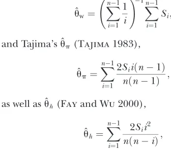
As our basic summary statistics, we choose Watterson’s estimator (Watterson1975),
ˆ
uw¼ Xn1 i¼1 1 i !1 Xn1 i¼1 Si;
and Tajima’s ˆup(Tajima1983),
ˆ
up¼ Xn1
i¼1
2Siiðn1Þ nðn1Þ ; as well as ˆuh(Fayand Wu2000),
ˆ
uh¼X n1
i¼1 2Sii2 nðniÞ;
whereSiis the number of derived variants founditimes in a sample ofnchromosomes.
We furthermore consider Tajima’sD(Tajima1989b) and Fay and Wu’sH(Fayand Wu2000; Zenget al. 2006) that both combine the information of two of the above-mentioned summary statistics. Therefore they both are somewhat redundant. As a measure of linkage disequi-librium, we add the integrated extended haplotype homozygosity, iHH (Sabeti et al. 2002; Voight et al. 2006).
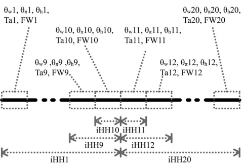
2 kb. Whereas ˆuw, ˆup, ˆuh, Tajima’sD, and Fay and Wu’sH
are calculated separately for each subsegment, iHH is computed from the center up to a distance of 2, 4,. . ., 20 kb separately on each side. As shown in Figure 1, iHH is first computed by integrating from the starting point of the sequence up to 20 kb. The result is denoted by iHH1. Next iHH2 uses the window from 2 kb up to 20 kb. The final iHH statistic for the left-hand part is iHH10, going from 18 kb up to 20 kb. For the right-hand part of the sequence extending from 20 kb up to 40 kb, 10 values of iHH are obtained analogously.
Simulation: Both for training and for testing, we simulated scenarios involvingn¼10 sequences each of lengthl¼40 kb with a recombination rate ofr¼0.02. We chose several different values foraand the timet
since the beneficial mutation became fixed (in units of 2Ngenerations) when simulating selection samples and assumed that the beneficial site is located in the middle of the sequence (Bsite ¼ 20 kb). For each set of parameters, 500 neutral samples and 500 selection samples were simulated as a training data set. The same sample size was also used for the test data.
We considered two different mutation schemes: (1) a fixed mutation rateu¼4Nm¼0.005 and (2) a fixed number of segregating sites (K ¼ 566, which is the expected number of segregating sites under neutrality whenu¼0.005; see Watterson1975). In practical ap-plications, the second mutation scheme corresponds to a strategy where, under both scenarios, one generates training samples with the number of segregating sites being equal to that observed for the actual data.
To simulate neutral samples and samples under selection, we used the SelSim (Spencerand Coop2004) software. Bottleneck samples were simulated via the ms program of Hudson(2002). The mbs program by Teshima and Innan (2009) was adapted to simulate
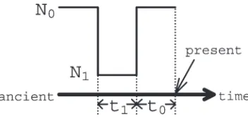
selective sweeps that occurred with bottlenecks. The simulation parameters and some notation are summa-rized in Table 1 and Figure 2.
Controlling the type I error: By default, boosting treats type I and type II errors symmetrically and predicts thatY¼1, iff(X).g¼0.5. If one desires to control the type I error probability under a null model such as neutrality, this can be achieved by adjusting the threshold
g. For this purpose, we first obtain a boosting classifier on the basis of training samples as usual. Then we generate 500 independent training samples under the null model and chooseg such that 95% of these samples are clas-sified correctly. To investigate the efficiency of the result-ing classifier under the alternative model, we generated 500 further independent test samples.
Figure1.—Predictor variables used as inputXto boosting.
Ta, Tajima’sD; FW, Fay and Wu’sH. We cut up the whole re-gion (40 kb) into 20 subsegments, each of length 2 kb. For each subsegment, we compute ˆuw, ˆup, ˆuh, Tajima’s D, and
Fay and Wu’s H. Overlapping subsegments are used with iHH. In total, this leads to 6320¼120 predictor variables that are used as input vectorXto boosting.
TABLE 1
Parameters and terminology
General parameters
n The number of sequences in the sample l The length of the investigated region u u¼4Nm, the population mutation rate per
nucleotide, whereNis the effective population size for a diploid population, andmis the mutation rate per nucleotide per generation
K Number of segregating sites in a sample r r¼4Nr, the population recombination rate
per nucleotide, whereris the recombination rate per nucleotide per generation
Selection parameters
a a¼2Ns, the selective strength, wheresis the selective advantage of the beneficial allele over the ancient allele
t Time since the beneficial mutation became fixed, in units of 2Ngenerations
Bsite Distance between the beneficial site and the left end of the sequenced region
Bottleneck parameters (see Figure 2) t0 Time since end of bottleneck, in units of
2Ngenerations
t1 Duration of bottleneck, in units of 2Ngenerations
D D¼N1/N0, depth of bottleneck N0 Effective population size before and
after bottleneck
N1 Effective population size during bottleneck
Notation
neu 500 simulated neutral samples
sel(a,t) 500 simulated selection samples with givena andt
bot(t0,t1) 500 simulated bottleneck samples with given t0andt1
N(a,b2) Gaussian distribution, wherea¼mean and
b2¼variance
RESULTS
Discriminatory power:According to Figure 3, all our summary statistics, except for iHH, show a valley pattern under the selection scenario only. For iHH, the in-tegration causes a valley both for the neutral and for the selection case. However, there are still differences in level and shape under the two competing scenarios.
We first investigate samples generated under the same values foraandtboth for training and for testing. The results in Table 2 show that our method is quite efficient in distinguishing neutrality from selection. Even when the selective sweep is weak and old (a¼200 andt¼0.2), we get an accuracy of 88.0% under a fixed value ofu. See Li and Stephan(2006) for a categorization of strong and weak selection in Drosophila.
In practice this approach is too optimistic, since the parameters of the selection scenario are usually un-known. One more practical strategy is to do the training over a whole range of parameter values, representing the prior belief concerning possible parameter values. For this purpose we use samples generated under pa-rameters chosen from a normal prior distribution with support restricted to the range of possible parameter values. We also generated parameters from a uniform distribution with very similar results (seeTable S1). To facilitate interpretation, testing is usually done with samples generated under fixed parameter values. Not unexpectedly, training our classifier with samples gen-erated under randomly chosen parameter values leads to some decrease in accuracy. According to Table 2, however, the power is still 87.6% in the most difficult test case (a¼200,t¼0.2, with fixedu).
If the alternative scenario is misspecified, our method seems to be quite robust at least in the situations we considered. When we trained the classifier with strong (a¼500) and recent (t¼0.001) selection but tested on a weak (a¼200) and old (t¼0.2) sweep, or vice versa, the power of the boosting classifier remains quite high (see the last two rows in Table 2).
Sinceuis often unknown in practice and may also vary for reasons other than selection, an option is to simulate training data for the two competing scenarios under a
fixed number of segregating sitesKthat equals the one seen in the actual test data. With this strategy, boosting is still able to learn the valley pattern. Obviously the exclusion of information concerning differences in the overall value of u will lead to some decrease in power. Table 2 illustrates the amount of power lost. Among our considered scenarios, the predictive power turned out to be.75% in all cases.
The results are for boosting with the L2fm loss function (Bu¨ hlmann and Hothorn 2007). Using a different loss function does not affect the results much. (SeeTable S2andTable S3.)
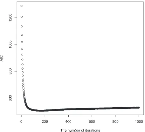
We also studied the use of AIC as a stopping rule for our boosting iterations. A typical example is provided in Figure 4. As the number of iterations increases, AIC decreases very rapidly at first, and then slows down, maintaining a steady level for a long period. In the example, the lowest AIC value is obtained at the 175th iteration. Stopping at the 1000th or 10,000th iteration led to almost the same predictive accuracy (results not shown), providing empirical support for the slow over-fitting of boosting.
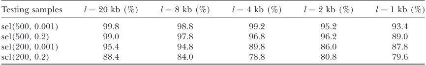
Another quantity influencing the predictive accuracy is the sequence length. In Table 3, we investigate the decrease in power when the available sequences have a length,40 kb, the length considered so far. The results suggest that the decrease in power is not dramatic even when going down until sequences of length 1 kb.
Boosting-based genome scans: It turns out that the boosting classifier is quite specific with respect to the position of the selected site. When training the classifier with the selected site at 20 kb, the power decreases quickly, if the position of the selected site is moved away from this position in the testing samples (Table 4). This can be exploited in the context of genome scans for selection. Indeed, if sufficiently large sequence chunks are avail-able, it is possible to slide a window consisting of our 20 subsegments along the sequence. A natural estimate of the position of the selected location is then the center of the window with the strongest evidence for selection.
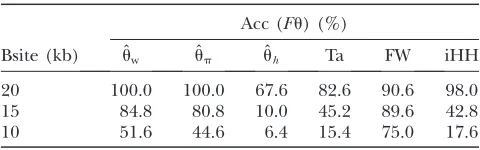
To learn which summary statistics are most specific with respect to the selected position, we investigate them separately by applying the boosting classifier on the basis of just one of the summary statistics at a time. It turns out that the effect of smaller deviations from the hypothetical selected site is particularly strong for ˆuh, Tajima’s D, and iHH (Table 5). One might therefore want to increase the specificity to position by using only ˆuh, Tajima’sD, and iHH. See Figure 5 for an ex-ample of a genome scan based on these three summary statistics.
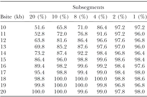
If a longer chromosome region is not available, or if a high specificity with respect to location is not desired, the specificity of the method can be reduced by cutting the sequences into fewer subsegments of larger size (Table 6), which intuitively smoothes the valley pattern. Figure2.—Terminology for bottleneck scenarios. A
Since the range of influence of a selective sweep depends on the strength of selection (a), the sensitivity of the classifier with respect to spatial position depends also ona. The smallerais, the narrower the affected nearby region and the higher the sensitivity with respect to the assumed position of the sweep.
Sensitivity toward bottlenecks: Demography leaves traces in genomic data similar to those caused by selective events (Tajima1989a,b), making it difficult to distinguish between these competing scenarios (Schlo¨ tterer2002; Schmidet al. 2005; Hamblinet al. 2006; Thorntonand Andolfatto 2006). To investigate how often selective sweeps and bottlenecks are confounded, we applied the boosting classifier, previously trained on neutral and selective sweep samples, and tested it on bottleneck samples. When simulating bottleneck samples, we fixed D¼0.01, and tried different values oft0andt1.
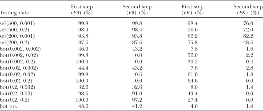
When training under neutrality and selection with fixed identical values foru, bottlenecks and sweeps cannot be distinguished reliably [see the ‘‘First step (Fu)’’ column in Table 7]. The reason is that a reduced number of segregating sites is observed both under bottlenecks and under sweeps but not under neutrality. One way to avoid this is to train the boosting classifier conditional on the observed number of segregating sites. With this strategy, the number of misclassifications (i.e., classifying a bottle-neck as a sweep) goes down considerably [see the ‘‘First step (FK)’’ column in Table 7].
To make our method even more specific, we propose a two-step method, which is in the spirit of Thornton
and Jensen (2007). For this purpose, we use two clas-sifiers (C), denoted by C1 and C2. C1 is trained under neutralityvs.selection, whereas C2 is under bottleneck vs.selection. For a test sample, we first apply C1. If se-lection is predicted, then we use C2, to classify between selection and bottleneck. The results [see in particular the ‘‘Second step (FK)’’ column in Table 7] indicate that this approach is quite efficient in the sense that misclas-sifications of bottleneck samples were very rare. On the other hand, the price for this is a somewhat decreased power of sweep detection when K is chosen equal in training and testing.
If a bottleneck sample and a selection sample are similar such that they produce similar overall values of a certain summary statistic, our method still works. In fact, the fixation of K implies that ˆuw is identical both for
selection and for bottleneck samples when computed over the whole sequence. Ignoring subsegments, we also generated selection and bottleneck samples with an identical average value of the overall ˆup. This was done by first generating sel(500, 0.001) samples and then choosing the bottleneck parameterD to get the same value of ˆup under both scenarios. It turned out that even in this situation the false positive still remained low (see the ‘‘Bot no.’’ line in Table 7).
Comparison with other methods:Currently there are several methods available to identify genomic regions affected by selection. Our main focus has been on comparing boosting with other approaches that also combine different pieces of information. More specif-Figure3.—Spatial patterns of summary
ically, we considered both summary statistic-based ap-proaches and the support vector machine approach of Pavlidis et al. (2010) that combines site frequency information [SweepFinder (Nielsen et al. 2005)] with linkage disequilibrium information [v-statistic (Kim and Nielsen 2004)]. Further approaches, which we did not consider here, include the composite-likelihood method of Kim and Stephan (2002) and selection scans based on hidden Markov models (Boitardet al. 2009).
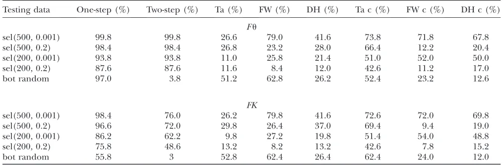
As tests that use summary statistics, we considered Tajima’s D(Tajima 1989b) and Fay and Wu’sH(Fay and Wu2000), as well as their combined form, theDH test (Zenget al. 2006). We calibrated all methods to give a type I error probability of 5% and then applied them to the same test data sets. In Table 8, we provide a comparison of the predictive accuracy between boosting and the above-mentioned methods that use summary statistics. We consider different selection scenarios, as well as bottleneck scenarios with randomly chosen parameters. Boosting always distinguished better be-tween neutrality and selection than the other three methods. While one-step boosting often interpreted bottlenecked samples as evidence for selection, even when the DHtest did not, the two-step boosting al-gorithm has a much better specificity than the DH test.
Since the above-mentioned test statistics were com-puted only once across the whole 40-kb region, one might wonder whether the selective signal was weak-ened due to an averaging effect. We therefore recom-puted the test statistics using only the center section of the region. This improved the performance of the test
statistics, but boosting still performed better (Table 8). While theDHtest that uses only the central window did better than the version using the whole sequence information, two-step boosting still provided the highest specificity toward bottlenecks. While two-step boosting can easily distinguish almost all the bottleneck events from selection, it can still recognize at least 87.6% of true selection events whenuis fixed and 75.8% whenK is fixed (Table 8).
Additionally, we compared our method with another recently published method developed by Pavlidiset al. (2010). The method uses support vector machines, another machine learning method, to combine a site frequency-based statistic obtained from SweepFinder with thev-statistic that measures linkage disequilibrium. We first investigated the behavior when distinguish-ing neutrality from selection and also bottlenecks from selection. For our simulations, we used the same pro-gram ssw (Kim and Stephan 2002) as Pavlidis et al. (2010) and chose identical parameters (n ¼ 12, l ¼ 50 kb, Bsite¼25 kb,r¼0.05). The bottleneck samples were simulated with ms (Hudson 2002). For further parameters please refer to Table 9. To permit for a fair comparison, we followed Pavlidiset al. (2010) and used the same parameters for both training and testing. The results (Table 9) show that our method performs better under all considered scenarios.
Our next comparison with Pavlidis et al. (2010) involves a class of scenarios where a selective sweep Figure4.—AIC. A typical AIC curve from a boosting run
(500 neutral samples and 500 selection samples with a ¼ 200, t¼0.2, and fixedu) is shown. Thex-axis indicates the number of iterations and they-axis the value of AIC. At the 175th iteration AIC reached its minimum. We can see that AIC decreases very fast at first, but changes only very slowly later on, which is in accordance with the slow overfitting fea-ture of boosting.
TABLE 2
Performance of boosting under different training strategies
Training data Testing data
Acc (Fu) (%)
Acc (FK) (%)
neu1sel(500, 0.001) sel(500, 0.001) 100.0 100.0 neu1sel(500, 0.2) sel(500, 0.2) 99.4 96.4 neu1sel(200, 0.001) sel(200, 0.001) 98.6 97.8 neu1sel(200, 0.2) sel(200, 0.2) 88.0 82.2 neu1sel(N(500, 2002),
N(0.2, 0.12))
sel(500, 0.001) 99.8 98.4
sel(500, 0.2) 98.4 96.6 sel(200, 0.001) 93.8 86.2 sel(200, 0.2) 87.6 75.8 neu1sel(500, 0.001) sel(200, 0.8) 86.6 77.2 neu1sel(200, 0.8) sel(500, 0.001) 100.0 99.6
happened within a bottleneck. We again simulated under identical parameters (n¼12,l¼50 kb, Bsite¼25 kb,r¼ 0.01) and used the same software mbs (Teshima and Innan 2009) to generate data. The results as well as further implementation details are shown in Table 10. Our method always provided better results in terms of both false positives (FP) and accuracy (Table 10).
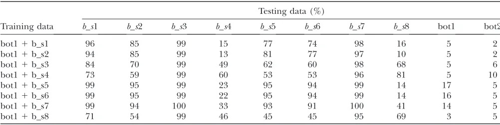
To avoid a too optimistic picture of the performance in practice, we also present cross-testing results where training and testing parameters differ. The FP rates have been adjusted to 0.05 (Table 11). When testing for old sweeps (older than the bottleneck) (b_s4 andb_s8) while training with other scenarios, or vice versa, the power tends to be low. Classification tends to be particularly difficult in cases where the selective sweep happened much earlier than the bottleneck (seeb_s4 andb_s8), and an explanation might be that the signal of the sweep gets diluted by the bottleneck event.
In many situations, however, the power remains at an acceptable level, indicating to some extent the robust-ness of our method.
We also checked the robustness of the false positive rate with respect to the null scenario. For this purpose we again adjusted the boosting classifier to get a false positive rate of 5% under the null training scenario. When training is done under short and deep bottlenecks (bot1), long and shallow bottlenecks (bot2) without a simultaneous selective sweep are rarely misclassified and the false positive rate remains small except for bot11 b_s4, where the sweep happened much earlier than the bottleneck (Table 11). The results in the opposite direction are less robust: Under training with long and shallow bottlenecks (bot2), short and deep bottlenecks (bot1) lead more frequently to false signals of selection. Depending on the specific alternative scenario used for training, we get false positive rates between 3 and 17% (Table 11).
As a further check for robustness, we trained under bottleneckvs. selection but tested on selection within a bottleneck without adjusting the false positive rate. Compared to the results shown in Table 10, the power
decreases inb_s4 andb_s8, but remains higher than the one obtained by Pavlidis et al. (2010) in most cases. Detailed results can be found in Figure 12.
Application to real data: We applied boosting to a small region of the maize genome. We follow an analysis by Tian et al. (2009), where they investigate 22 loci spanning 4 Mb on chromosome 10 and identify a selective sweep that affected this region. We imple-mented the two-step method and used the real sequence data as our testing data. For training, we simulated samples under the parameters estimated in Tianet al. (2009). We used in particular the estimated mutation rateu ¼0.0064 and the estimated recombination rate
r¼0.0414.
We chose to investigate 12 of their 22 loci located at 85.65 Mb on chromosome 10, each of length 1 kb. Since the number of individuals varied slightly from 25 to 28 between the loci (Tianet al. 2009), we simply setn¼25. Training data under selection were generated with parameters chosen randomly according to sel(N(500, 2002),N(0.2, 0.12)).
According to previous studies, maize experienced a bottleneck event and the bottleneck parameter k (population size during bottleneck/duration of bottle-neck in units of generations) was 2.45 (Wrightet al. 2005; Tianet al. 2009). We sett0¼0.02 andt1¼0.02 (in units of 2N generations, where N is the effective population size). We then chose D ¼0.098 such that D3N/(t132N)¼2.45.
In Tian’s article, ˆup, ˆuw, and Tajima’s D were
com-puted for each locus (values at certain loci were un-available). We used these three statistics and ignored missing values. Then we applied the two-step method using the L2fm loss. The threshold between neutrality (Y¼0) and selection (Y¼1) was 0.462, and the first-step result wasf¼1.382; sincef?0.462, this provides strong evidence for selection. The threshold between bottle-neck (Y¼0) and selection (Y¼1) was 0.407, and the second-step result was 4.700, indicating that the signal at the considered locus cannot be explained by a bottle-neck only. The result supports the findings in Tianet al.
TABLE 3
Detection power in dependence of the sequence length
Testing samples l¼20 kb (%) l¼8 kb (%) l¼4 kb (%) l¼2 kb (%) l¼1 kb (%)
sel(500, 0.001) 99.8 98.8 99.2 95.2 93.4
sel(500, 0.2) 99.0 97.8 96.8 96.2 89.0
sel(200, 0.001) 95.4 94.8 89.8 86.0 87.8
sel(200, 0.2) 88.4 84.0 78.8 80.8 79.6
We consider samples of sequences of lengthland fixeduto the same value in training and testing. Train-ing was done with neu1sel(N(500, 2002),N(0.2, 0.12)). The type I error probability (probability of
(2009), where a selective sweep was also identified. There a was estimated to be 22187.8, which is much larger than the value we used in our training data generated from (N(500, 2002)).
Learning about the relative importance of summary statistics:One advantage of the version of boosting we used is that the approach leads to coefficients for each of the considered summary statistics. The coefficients can be used to measure the relative importance of each summary statistic. It is important to standardize the coefficients, since otherwise the estimated coefficients will depend on the scale of variation of the respective summary statistics. For the jth component of the pre-dictor variable, X(j), the coefficient is ˆbð Þj , and the
standardized coefficient is ˆbð ÞjpffiffiffiffiffiffiffiffiffiffiffiffiffiffiffiffiffiffiffiffiVaˆrðXð Þj Þ. The impor-tance of a statistic is indicated by the absolute value of its standardized coefficient. The closer a coefficient is to zero, the smaller the contribution of the statistic to the classifier. To make the results fairly independent of the randomness of an individual data set, we report the average coefficients over 10 trials, with each trial involving boosting with 500 neutral (or bottleneck) samples and 500 selection samples.
When considering the statistics at all positions simul-taneously, the relative importance will depend on two components: the relative importance of different posi-tions and the relative importance of different statistics. To get a clearer picture, we consider the different sub-segments separately and use the boosting classifier on the information of only one subsegment at a time. The re-sults can be found in Figure 6. Because iHH uses not only local information (see Figure 1), the information content for a given subsegment is higher than that for other summary statistics, especially at the border subsegments.
Figure 6 provides the standardized coefficients for several scenarios. Here, we note some observations concerning the patterns shown in Figure 6:
1. For classifying between neutrality and selection, ˆup plays an important role, consistently over all
scenar-ios. On the other hand, ˆuw plays a role only when
selection happened recently, but not for old sweeps. A reason might be that the occurrence of new mu-tations after selection makes the relative amount of low-frequency mutations increase. But as age increases, some low-frequency mutations drift to intermediate-frequency mutations, and thus the proportion of low-frequency mutations decreases. Since ˆuwshould be more affected by such low-frequency mutations than ˆup (Fayand Wu2000), ˆuwbecomes less important when selection gets older.
2. When discriminating against a neutral scenario, the iHH statistic seems particularly important for recent selective sweeps. If the fixation of the beneficial allele happened a longer time ago, the iHH statistic is much less important. A possible explanation is that the LD is then broken up by recombination or by the recurrent neutral mutations that occur after the fixation of the beneficial mutation.
3. When discriminating between bottlenecks and selec-tion, ˆuw seems most important, and its importance increases toward the border of the observation region. This indicates a larger difference in the number of low-frequency mutations between bottle-necks and selection farther away from the beneficial mutation. Linkage disequilibrium tends to contrib-ute less in such a setup.
4. We also investigated the situation for samples where the number of mutations K is fixed (Figure 7). Compared with the previous samples where u was fixed (Figure 6), there is not much difference when distinguishing between neutrality and selection. When classifying between bottleneck and selection, however, we observe differences. Since the overall number of segregating sites is now the same for the two scenarios, the classifier uses the spatial pattern of variation, leading to the spatial pattern of the coefficients shown in Figure 7.
TABLE 4
Accuracy depending on the position of the selected site
Bsite (kb) Acc (Fu) (%)
20 100.0
15 80.6
10 44.2
Training was done with neu1sel(500, 0.001) and Bsite¼ 20 kb, and the type I error probability was adjusted to 5%. Testing was done on sel(500, 0.001) with different positions Bsite of the beneficial mutation. It can be seen that the sweep detection power decreases quickly with increasing distance of the positions of the selected site between training and testing samples. Acc: percentage of cases where a sweep is detected. See Table 1 for details of the notation.
TABLE 5
Accuracy depending on the position of the selected site for different summary statistics
Acc (Fu) (%)
Bsite (kb) uˆw ˆup uˆh Ta FW iHH
20 100.0 100.0 67.6 82.6 90.6 98.0
15 84.8 80.8 10.0 45.2 89.6 42.8
10 51.6 44.6 6.4 15.4 75.0 17.6
We show the power of detecting a selective sweep depend-ing on the position Bsite of the selected site. To investigate the sensitivity of the individual statistics with respect to position, we used only one of the mentioned statistics at a time both in training and in testing. We trained with neu1sel(500, 0.001), Fu, and Bsite¼20 kb and adjusted the type I error probability to 5%. ˆuh, Tajima’sD, and iHH are particularly sensitive to the
DISCUSSION AND CONCLUSION
Boosting is a fairly recent statistical methodology for binary classification. It permits one to efficiently com-bine different pieces of evidence to optimize the performance of the resulting classifier. In population
genetics, a natural choice for such pieces of evidence is individual summary statistics. By choosing an appropri-ate boosting method, one can actually learn about the relative importance of different summary statistics by looking at the resulting optimized classifier. For sum-mary statistics that are otherwise difficult to combine (such as site frequency spectrum and LD measures), this seems to be particularly interesting.
It is well known that single population genetic sum-mary statistics are usually not sufficient. For methods such as ABC that rely on inference from summary statistics, an important issue is the choice and/or combination of summary statistics to obtain precise estimates. A promis-ing approach seems to be to use boostpromis-ing as a first step: The situation remains challenging, though, since differ-ent summary statistics could in principle be important in different parameter ranges.
Although boosting could be applied for any set of competing population genetic scenarios, we focused on the detection of selective sweeps both within a bottle-neck and within a neutral background. Such scenarios have been fairly well studied and several methods have already been proposed. It is therefore possible to judge the performance of boosting, given what is known about the performance of other methods. Our simulation results indicate that boosting performs better than other summary statistic-based methods. This indicates that boosting is able to come up with efficient com-Figure 5.—Boosting-based genome scans. In each of the
three diagrams, each column represents an independently simulated 100-kb chromosome region where a beneficial mu-tation (a¼500,t¼0.001) occurred. The rows indicate the position within the sequence. The dot to the right of each graph marks the position 50 kb where the beneficial mutation occurred. Within a column, each pixel indicates the classifica-tion result based on a 40-kb window sliding along the chromo-some region (step length 2 kb). Training was done with neu1
sel(500, 0.001). A solid pixel indicates that boosting predicted the considered position to have experienced a selection event. As desired, the solid pixels are concentrated at the se-lected position. In the top diagram, six different summary sta-tistics were used, whereas in the middle diagram, only ˆuh,
Tajima’sD, and iHH were used. The type I error probability was adjusted to 5% in both cases. In the bottom diagram, the same six summary statistics were used as in the top dia-gram, but the type I error probability was reduced to 0.2%, corresponding to a threshold of g ¼ 0.5 for the boosting classifier. Both using position-specific summary statistics and decreasing the type I error probability lead to decreased false positive rates in a genome scan.
TABLE 6
Accuracy with respect to the number of subsegments
Subsegments
Bsite (kb) 20 (%) 10 (%) 8 (%) 4 (%) 2 (%) 1 (%)
10 51.6 65.8 71.0 86.4 97.2 97.2
11 52.8 72.0 76.8 91.6 97.2 96.0
12 63.8 81.6 86.4 96.6 97.6 96.8
13 69.8 85.2 87.6 97.6 97.0 96.0
14 73.2 87.4 92.2 98.4 96.8 96.4
15 86.4 96.0 98.8 99.6 98.6 98.4
16 89.4 98.2 99.6 99.2 98.4 97.6
17 95.4 98.8 99.4 99.0 98.4 98.0
18 98.8 100.0 100.0 100.0 98.8 98.6
19 99.8 100.0 100.0 99.8 96.8 96.8
20 100.0 100.0 99.6 99.0 97.8 98.0
binations of summary statistics. We also applied boost-ing to the scenarios in Pavlidis et al. (2010), where the authors used support vector machines (SVMs) to combine the composite likelihood-ratio statistic ob-tained from a modified version of the SweepFinder software (Nielsenet al. 2005) with a measure of linkage disequilibrium. For sweeps both within and without bottlenecks, boosting usually provided a higher power of detection while the false positive rate was equal or lower.
Using a sliding-window approach, boosting may also provide a way to carry out genome scans for selection.
So far, our focus has been on an ideal situation where both the mutation rate and the recombination rate were constant; we considered only completed selective sweeps and no alternative types of selection; the population size was taken as either constant or affected by a bottleneck. However, in reality, a much more complex population history may have left its traces in our summary statistics, influencing the accuracy of our method. On the basis of knowledge from the current literature, we discuss how to carry out boosting-based scans for selection in the presence of such additional factors. Further simulations are needed to confirm our suggestions:
Mutation heterogeneity: We considered regions of length 40 kb. If the mutation rates are heterogeneous within such a segment, this can lead to reduced values ofupandKand a positive Tajima’sD, depending on
how severe the heterogeneity is (Aris-Brosou and Excoffier 1996). If the extent of heterogeneity is large, this may lead to false detections of selection, since a reduced up and a reduced K are also encountered under positive selection. If one suspects mutation rate heterogeneity as a possible alternative explanation for a positive classification result, one may try to resolve the issue by training the boosting classifier with mutation rates that vary from site to site according to a gamma distribution (Uzzell and Corbin1971; Aris-Brosouand Excoffier1996) to mimic mutation heterogeneity. On a genomic scale, the mutation rate may also vary. Scanning the whole genome with a classifier that has been trained under one single mutation rate may then give misleading re-sults. Think, for instance, of a classifier that has been trained under a high mutation rate but is subse-quently applied to DNA segments where the mutation rate has been much lower. A low level of polymor-phism may then be viewed as a signal of selection. One possible solution is to divide the whole genome into segments and to scan each segment indepen-dently with a classifier that is trained under an ap-propriate mutation rate. Another approach that we investigated in this article is to carry out training under the same numberKof mutation events that is observed at the currently scanned genome segment.
TABLE 7
Rate of predicting selection with bottlenecks as an alternative scenario
Testing data
First step (Fu) (%)
Second step (Fu) (%)
First step (FK) (%)
Second step (FK) (%)
sel(500, 0.001) 99.8 99.8 98.4 76.0
sel(500, 0.2) 98.4 98.4 96.6 72.0
sel(200, 0.001) 93.8 93.8 86.2 62.2
sel(200, 0.2) 87.6 87.6 75.8 48.6
bot(0.002, 0.002) 46.0 43.2 7.8 1.6
bot(0.002, 0.02) 99.8 0.0 56.0 2.2
bot(0.002, 0.2) 100.0 0.0 30.2 0.4
bot(0.02, 0.002) 44.4 43.2 7.8 2.8
bot(0.02, 0.02) 99.8 0.6 61.6 1.8
bot(0.02, 0.2) 100.0 0.0 64.6 0.0
bot(0.2, 0.002) 32.6 32.6 8.0 1.4
bot(0.2, 0.02) 98.6 91.0 49.4 0.0
bot(0.2, 0.2) 100.0 97.2 27.4 0.0
bot no. 48.6 41.2 4.0 1.4
We investigate how often selection is predicted by the two-step boosting classifier discussed inSensitivity toward bottlenecks. For selection scenarios, these cases contribute true positives; for bottleneck scenarios, they are false positives. First step, the percentage of testing samples classified as selection by classifier (C)1; second step, the percentage of testing samples classified as selection by both C1 and C2. C1 was trained with neu1sel(N(500, 2002),N(0.2, 0.12)) and the type I error probability was adjusted according to 500 independent neutral samples.
C2 was trained under bot(N(0.02, 0.012),N(0.02, 0.012))1sel(N(500, 2002),N(0.2, 0.12)) and the type I error
probability was adjusted according to 500 independent bot(N(0.02, 0.012),N(0.02, 0.012)). Bot no. indicates
that the bottleneck samples have the same average ˆup-value (computed once across the whole region) as
Recombination heterogeneity: In the human genome, for instance, there is a recombination hotspot of length 1 kb approximately every 100 kb of sequence
(Kauppi et al. 2004; Calabrese 2007). If the inves-tigated region contains recombination hotspots, this will reduce the LD and may consequently reduce the
TABLE 8
Comparison of boosting with other summary statistic-based methods
Testing data One-step (%) Two-step (%) Ta (%) FW (%) DH (%) Ta c (%) FW c (%) DH c (%)
Fu
sel(500, 0.001) 99.8 99.8 26.6 79.0 41.6 73.8 71.8 67.8
sel(500, 0.2) 98.4 98.4 26.8 23.2 28.0 66.4 12.2 20.4
sel(200, 0.001) 93.8 93.8 11.0 25.8 21.4 51.0 52.0 50.0
sel(200, 0.2) 87.6 87.6 11.6 8.4 12.0 42.6 11.2 17.0
bot random 97.0 3.8 51.2 62.8 26.2 52.4 23.2 12.6
FK
sel(500, 0.001) 98.4 76.0 26.2 79.8 41.6 72.6 72.0 69.8
sel(500, 0.2) 96.6 72.0 29.8 26.4 37.0 69.4 9.4 19.0
sel(200, 0.001) 86.2 62.2 9.8 27.2 19.8 51.4 54.0 48.8
sel(200, 0.2) 75.8 48.6 13.2 8.2 13.2 42.6 7.8 15.2
bot random 55.8 3 52.8 62.4 26.4 62.4 24.0 12.0
The percentage of times selection was predicted for testing samples that were simulated under different selective and bottleneck scenarios is shown. We compared the following approaches that use summary statistics: Ta, Tajima’sD; FW, Fay and Wu’sH; DH, DH test; c, center. First, these statistics were computed only once across the whole 40-kb region, which may lead to a weakened selective signal according to an averaging effect. Since the signal in the center of the region will usually be the strongest, we then tried to use only the 4-kb center section of the region to compute the statistics. The results can be found under Ta c, FW c, and DH c. ‘‘One-step’’ and ‘‘two-step’’ indicate one-step boosting and two-step boosting, respectively. These results are the same as in Table 7. bot random¼bot(N(0.02, 0.012),N(0.02, 0.012)). The type I error probability of boosting (both for one-step and for two-step) was
adjusted to 5%, and we chose cutoff points for the other tests also according to the 5% quantile estimated from 50,000 simulated neutral samples. The samples were generated under both fixedu(Fu) and fixedK(FK). We can see that boosting always performed much better for distinguishing neutrality from selection, although the difference between the methods was reduced slightly when Tajima’sD, Fay and Wu’sH, and the DH test were calculated only from the center section of the region. Under the more difficult situations the advantage of boosting is particularly visible. Note that one-step boosting predicted most of the bottleneck samples as selection whereas the DH test did not. The application of two-step boosting, however, solved this problem.
TABLE 9
Comparison of boosting with the method proposed by PAVLIDISet al.(2010) under neutrality and bottlenecksvs. selective sweeps
Training data Testing data FP (%) Acc (%) Pavlidis’s FP (%) Pavlidis’s Acc (%)
neu11sel1 sel1 0 98 3 90
neu21sel2 sel2 0 100 0 98
bot11sel1 sel1 1 100 26 75
bot21sel2 sel2 0 99 18 84
sel1, sel(500, 0.0001); sel2, sel(2500, 0.0001). To make the setup equal to that in Pavlidiset al.(2010), we
generated 2000 training samples for each parameter set. (The results were almost identical when we followed our standard training procedure and used only 500 training samples.) Both sel1 and sel2 were generated under u¼0.005. For each sample taken according to sel1, we computed Watterson’s estimate ˆuw(Watterson1975) and generated a neutral sample withu¼uˆw. The training data neu1 consisted of 2000 neutral samples obtained in this way. We obtained neu2 analogously by matchinguto sel2. bot1 and bot2 were bottleneck samples with the parameters as in Liand Stephan(2006). This is a 4-epoch bottleneck model: Backward in time, a
bottle-neck happens from 0.0734 time units to 0.075 time units (in 2N0generations, whereN0is the current effective population size), and the population size reduces to 0.002N0, then instantly the population size changes to 7.5N0, and finally it becomes 1.5N0 at 0.279 time units. For each realization of sel1,uwas again estimated, and a corresponding bottleneck sample was obtained usingu¼ˆu. See Pavlidiset al. (2010) and Zivkovic
and Wiehe(2008) for details. Again bot1 consists of samples obtained in this way and bot2 was obtained
anal-ogously. FP, false positive rate; Acc, accuracy (power of detecting a selective event). The FPs of the four rows were computed according to neu1, neu2, bot1, and bot2, respectively. The samples of the same parameter set for training, testing, and FP computing were independently generated. The Pavlidis’s FP and Pavlidis’s Acc col-umns show the accuracy of the support vector machine-based method of Pavlidiset al. (2010). Rows 1 and 2 of
power of sweep detection. Nevertheless, since the other summary statistics that use polymorphism and site frequency spectrum information are not affected, the decrease in power may be limited. An obvious option would again be to take potential recombina-tion hotspots into account when training the boosting classifier.
Ongoing selection (incomplete sweeps): In our simu-lations, the beneficial mutation was fixed when the samples were taken. If selection is ongoing, the mutation frequency spectrum will be notably differ-ent from the one under neutrality when the
fre-quency of the beneficial allele reaches 0.6 (Zenget al. 2006). Thus there should be a chance to detect selection when the frequency of the beneficial allele is.0.6.
Recurrent selection: According to Pavlidiset al. (2010) recurrent selective sweeps will lead to a loss of the characteristic local pattern of selection events. On average, the sweep events will also often be quite old ( Jensenet al. 2007; Pavlidiset al. 2010). Both effects suggest that the power of detecting recurrent sweeps in a region will be somewhat lower than with a single selective event.
TABLE 10
Comparison of boosting with the method proposed by PAVLIDISet al.(2010): detecting a sweep within a bottleneck
Training data Testing data FP (%) Acc (%) Acc* (%) Pavlidis’s FP (%) Pavlidis’s Acc (%)
bot11b_s1 b_s1 8 98 96 51 71
bot11b_s2 b_s2 11 95 85 20 73
bot11b_s3 b_s3 0 98 99 8 97
bot11b_s4 b_s4 19 84 60 56 63
bot11b_s5 b_s5 6 97 95 27 50
bot11b_s6 b_s6 8 97 94 22 60
bot11b_s7 b_s7 2 99 100 35 67
bot11b_s8 b_s8 15 88 69 25 46
As in Pavlidiset al.(2010), we used a broad uniform prior foruand accepted only those realizations withK¼
50 both for training and for testing. We considered the following scenarios: bot1, bot(0.02, 0.0015),D¼0.002; bot2, bot(0.02, 0.0375),D¼0.05;b_s1,. . .,b_s8, selective sweep within a bottleneck with Bsite¼25,000 bp;b_s1, t0¼0.002,t1¼0.0015,D¼0.002,s¼0.002,t_mut¼0.02. Heresis the selective coefficient, andt_mut is the time when the beneficial allele occurred in the population. Note that all the time indicators in Pavlidis’s article are in the units of 4Ngenerations, but 2Ngenerations in this article.b_s2,t0¼0.02,t1¼0.0015,D¼0.002,s¼ 0.002,t_mut¼0.0214;b_s3,t0¼0.02,t1¼0.0015,D¼0.002,s¼0.8,t_mut¼0.0214;b_s4,t0¼0.02,t1¼0.0015, D¼0.002,s¼0.002,t_mut¼0.23;b_s5,t0¼0.02,t1¼0.0375,D¼0.05,s¼0.002,t_mut¼0.02;b_s6,t0¼0.02, t1¼0.0375,D¼0.05,s¼0.002,t_mut¼0.0214;b_s7,t0¼0.02,t1¼0.0375,D¼0.05,s¼0.1,t_mut¼0.0214; b_s8,t0¼0.02,t1¼0.0375,D¼0.05,s¼0.002,t_mut¼0.23. The other parametersn¼12,l¼50,000 bp, and
r¼0.01 are also chosen to match those in Pavlidiset al. (2010). For each parameter set, 2000 replications were
simulated. FP, false positive rate; Acc, accuracy (power of detecting a selective event). The false positive rate FP in rows 1–4 is under the bottleneck scenario bot1, whereas bot2 is used in rows 5–8. The results in Acc* provide the power when the false positive rate FP is adjusted to 0.05. The Pavlidis’s FP and Pavlidis’s Acc columns show the accuracy of the support vector machine-based method of Pavlidiset al. (2010). Rows 1–4 of these columns
are taken from Table 3 in Pavlidiset al. (2010), whereas rows 5–8 are from Table 4.
TABLE 11
Cross-testing: the power of detecting a sweep within a bottleneck if training and testing parameters do not coincide
Testing data (%)
Training data b_s1 b_s2 b_s3 b_s4 b_s5 b_s6 b_s7 b_s8 bot1 bot2
bot11b_s1 96 85 99 15 77 74 98 16 5 2
bot11b_s2 94 85 99 13 81 77 97 10 5 2
bot11b_s3 84 70 99 49 62 60 98 68 5 6
bot11b_s4 73 59 99 60 53 53 96 81 5 10
bot11b_s5 99 95 99 23 95 94 99 14 17 5
bot11b_s6 99 95 99 22 95 94 99 14 16 5
bot11b_s7 99 94 100 33 93 91 100 41 14 5
bot11b_s8 71 54 99 46 45 45 95 69 3 5
Background selection: Like positive selection, back-ground selection will also reduce the polymorphism level but it will not generate high-frequency mutations (Fu1997; Zenget al. 2006). If we train under neutrality vs. selection and the excess of low-frequency muta-tions is recognized by the classifier, it is possible that background selection will be wrongly identified as positive selection. To avoid this, a two-step method should be helpful. If a sample is classified as under selection, one may want to train the classifier using both positive selection and background selection samples in a second step. When using summary sta-tistics that measure the abundance of high-frequency mutations, we expect that the resulting classifier is able to distinguish between background and positive selection.
Balancing selection: If the equilibrium frequency of the selected allele is not very high, it is difficult to discover balancing selection. If on the other hand the equilib-rium frequency is fairly high (e.g., 75%) (Zenget al. 2006), the signature of balancing selection resembles that of positive selection. After the selected allele reaches its equilibrium frequency, some hitchhiking neutral alleles will also have high frequencies and will stay segregating for a longer period than under a selective sweep. This is because their frequency will be lower when reaching equilibrium, requiring more time for fixing them by drift (Zenget al. 2006). Thus our method should also detect balancing selection at high equilibrium frequency, and its age will affect the efficiency less than under positive selection.
Population growth: Population growth will cause an excess of low-frequency variants, but will not affect
high-frequency mutations (Fu1997; Zenget al. 2006). So like bottlenecks and background selection, a two-step method may be helpful to rule out population growth as an alternative explanation.
Population shrinkage: Population shrinkage will cause the number of low-frequency variants to be smaller than those of intermediate and high frequency (Fu 1996; Zeng et al. 2006). Since this is quite different from the signature caused by a selective sweep, we do not expect large problems for shrinking populations. Figure6.—The relative importance of different summary
statistics for the detection of selection under a fixed value ofu. Under different selective scenarios, we investigate the rel-ative importance of our summary statistics. One way of mea-suring their importance is in terms of the absolute value of the coefficients given to the summary statistics by the boosting classifier. A large coefficient means that a certain statistic is very influential at the considered position for our classifier. Each graph is based on an average of 10 trials, with each trial containing 500 neutral (or bottleneck) samples and 500 selec-tion samples. All the samples were generated with fixedu. The relative importance of the six summary statistics was consid-ered separately for each subsegment; that is, each time a boosting process was applied to only six statistics at a specific position.
TABLE 12
Training with selectionvs.bottleneck and testing with selec-tion within a bottleneck
Training data Testing data FP (%) Acc (%)
bot11sel1 b_s1 11 96
bot11sel2 b_s2 11 93
bot11sel3 b_s3 6 99
bot11sel4 b_s4 1 36
bot21sel5 b_s5 5 94
bot21sel6 b_s6 5 93
bot21sel7 b_s7 2 99
bot21sel8 b_s8 2 44
Population structure: When a population is structured, there may be an excess of low- or high-frequency derived alleles especially if the sampling scheme is unbalanced among the subpopulations (Zenget al. 2006). In addition, population structure may increase LD (Slatkin2008). This might obviously affect the results obtained from our boosting classifier and further research is needed to use boosting classifiers in the context of structured populations. AddingFstas
a summary statistic may obviously help in this context.
We thank Simon Boitard for helpful suggestions on the simulation process. We thank Simon Aeschbacher and the referees for helpful comments on the manuscript. We thank Pavlos Pavlidis for explaining the details of their parameter choices when simulating their SVM method. We also thank Kosuke M. Teshima for instructions on the program mbs. This work was financially supported by the Shanghai Pujiang Program (08PJ14104) and the Bairen Program. C.S. is supported by the Fonds zur Fo¨rderung der wissenschaftlichen Forschung, and A.F. was supported by Wiener-, Wissenschafts-, Forschungs- und Technologiefonds.
LITERATURE CITED
Akaike, H., 1974 A new look at the statistical model identification.
IEEE Trans. Automat. Contr.19(6): 716–723.
Aris-Brosou, S., and L. Excoffier, 1996 The impact of population
expansion and mutation rate heterogeneity on DNA sequence polymorphism. Mol. Biol. Evol.13(3): 494–504.
Beaumont, M. A., W. Zhangand D. J. Balding, 2002 Approximate
Bayesian computation in population genetics. Genetics 162:
2025–2035.
Biswas, S., and J. M. Akey, 2006 Genomic insights into positive
se-lection. Trends Genet.22(8): 437–446.
Boitard, S., C. Schlo¨ ttererand A. Futschik, 2009 Detecting
se-lective sweeps: a new approach based on hidden Markov models. Genetics181:1567–1578.
Breiman, L., 1998 Arcing classifiers (with discussion). Ann. Stat.
26(3): 801–849.
Breiman, L., 1999 Prediction games and arcing algorithms. Neural
Comput.11(7): 1493–1517.
Bu¨ hlmann, P., 2006 Boosting for high-dimensional linear models.
Ann. Stat.34:559–583.
Bu¨ hlmann, P., and T. Hothorn, 2007 Boosting algorithms:
regu-larization, prediction and model fitting. Stat. Sci.22(4): 477–505. Calabrese, P., 2007 A population genetics model with
recombina-tion hotspots that are heterogeneous across the popularecombina-tion. Proc. Natl. Acad. Sci. USA104(11): 4748–4752.
Fay, J. C., and C.-I. Wu, 2000 Hitchhiking under positive Darwinian
selection. Genetics155:1405–1413.
Freund, Y., and R. E. Schapire, 1996 A decision-theoretic
general-ization of on-line learning and an application to boosting. J. Comput. Syst. Sci.55(1): 119–139.
Fu, Y., 1996 New statistical tests of neutrality for DNA samples from a
population. Genetics143:557–570.
Fu, Y., 1997 Statistical tests of neutrality of mutations against
popu-lation growth, hitchhiking and background selection. Genetics
147:915–925.
Fu, Y., and W. Li, 1993 Statistical tests of neutrality of mutations.
Genetics133:693–709.
Grossman, S. R., I. Shylakhter, E. K. Karlsson, E. H. Byrne, S.
Moraleset al., 2010 A composite of multiple signals
distin-guishes causal variants in regions of positive selection. Science
327(5967): 883–886.
Hamblin, M. T., A. M. Casa, H. Sun, S. C. Murray, A. H. Paterson et al., 2006 Challenges of detecting directional selection after a bottleneck: lessons from sorghum bicolor. Genetics173:953– 964.
Han, J., and M. Kamber, 2005 Data Mining, Concepts and Techniques,
Ed. 2. Morgan Kaufmann, San Francisco.
Hothorn, T., and P. Bu¨ hlmann, 2002 Mboost: model-based
boost-ing. R package version 0.5-8. Available athttp://cran.r-project.org. Hudson, R. R., 2002 Generating samples under a Wright-Fisher
neu-tral model of genetic variation. Bioinformatics18(2): 337–338. Jensen, J. D., K. R. Thornton, C. D. Bustamanteand C. F. Aquadro,
2007 On the utility of linage disequilibrium as a statistic for identifying targets of positive selection in nonequilibrium popu-lations. Genetics176:2371–2379.
Joyce, P., and P. Marjoram, 2008 Approximately sufficient statistics
and Bayesian computation. Stat. Appl. Genet. Mol. Biol.7:26. Kauppi, L., A. J. Jeffreysand S. Keeney, 2004 Where the crossovers
are: recombination distributions in mammals. Nat. Rev. Genet.
5(6): 413–424.
Kim, Y., and R. Nielsen, 2004 Linkage disequilibrium as a signature
of selective sweeps. Genetics167:1513–1524.
Kim, Y., and W. Stephan, 2002 Detecting a local signature of genetic
hitchhiking along a recombining chromosome. Genetics 160:
765–777.
Li, H., and W. Stephan, 2006 Inferring the demographic history
and rate of adaptive substitution in Drosophila. PLoS Genet.
2:e166.
Nielsen, R., S. Williamson, Y. Kim, M. J. Hubisz, A. G. Clarket al.,
2005 Genomic scans for selective sweeps using SNP data. Genome Res.15(11): 1566–1575.
Pavlidis, P., J. D. Jensenand W. Stephan, 2010 Searching for
foot-prints of positive selection in whole-genome SNP data from non-equilibrium populations. Genetics185:907–922.
Sabeti, P. C., D. E. Reich, J. M. Higgins, H. Z. P. Levine, D. J. Richter et al., 2002 Detecting recent positive selection in the human ge-nome from haplotype structure. Nature419(6909): 832–837. Sabeti, P. C., S. F. Schaffner, B. Fry, J. Lohmueller, P. Varilly
et al., 2006 Positive natural selection in the human lineage. Sci-ence312(5780): 1614–1620.
Schlo¨ tterer, C., 2002 A microsatellite-based multilocus screen for
the identification of local selective sweeps. Genetics 160:753– 763.
Schmid, K. J., S. Ramos-Onsins, H. Ringys-Beckstein, B. Weisshaar
and T. Mitchell-Olds, 2005 A multilocus sequence survey in Arabidopsis thalianareveals a genome-wide departure from a neutral model of DNA sequence polymorphism. Genetics169:1601–1615. Schwarz, G., 1978 Estimating the dimension of a model. Ann. Stat.
6(2): 461–464.
Slatkin, M., 2008 Linkage disequilibrium—understanding the
evo-lutionary past and mapping the medical future. Nat. Rev. Genet.
9(6): 477–485.
Spencer, C. C. A., and G. Coop, 2004 Selsim: a program to simulate
population genetic data with natural selection and recombina-tion. Bioinformatics20(18): 3673–3675.
Figure7.—The relative importance of different summary
Tajima, F., 1983 Evolutionary relationship of DNA sequences in
fi-nite populations. Genetics105:437–460.
Tajima, F., 1989a The effect of change in population size on DNA
polymorphism. Genetics123:597–601.
Tajima, F., 1989b Statistical method for testing the neutral mutation
hypothesis by DNA polymorphism. Genetics123:585–595. Teshima, K. M., and H. Innan, 2009 mbs: modifying Hudson’s ms
software to generate samples of DNA sequences with a biallelic site under selection. BMC Bioinformatics10:166.
Thornton, K., and P. Andolfatto, 2006 Approximate Bayesian
infer-ence reveals evidinfer-ence for a recent, severe bottleneck in a Nether-lands population ofDrosophila melanogaster.Genetics172:1607–1619. Thornton, K. R., and J. D. Jensen, 2007 Controlling the false-positive
rate in multilocus genome scans for selection. Genetics 175:
737–750.
Tian, F., N. M. Stevensand E. S. BucklerIV, 2009 Tracking
foot-prints of maize domestication and evidence for a massive selec-tive sweep on chromosome 10. Proc. Natl. Acad. Sci. USA
106(Suppl. 1): 9979–9986.
Uzzell, T., and K. W. Corbin, 1971 Fitting discrete probability
dis-tributions to evolutionary events. Science172(988): 1089–1096.
Voight, B. F., S. Kudaravalli, X. Wenand J. K. Pritchard, 2006 A
map of recent positive selection in the human genome. PLoS Biol.4(3): e72.
Watterson, G. A., 1975 On the number of segregating sites in
ge-netical models without recombination. Theor. Popul. Biol.7(2): 256–276.
Wright, S. I., I. V. Bi, S. G. Schroeder, M. Yamasaki, J. F. Doebley et al., 2005 The effects of artificial selection on the maize ge-nome. Science308(5726): 1310–1314.
Zeng, K., Y. Fu, S. Shiand C.-I. Wu, 2006 Statistical tests for
detect-ing positive selection by utilizdetect-ing high-frequency variants. Genet-ics174:1431–1439.
Zeng, K., S. Shiand C.-I. Wu, 2007 Compound tests for the
detec-tion of hitchhiking under positive selecdetec-tion. Mol. Biol. Evol.
24(8): 1898–1908.
Zivkovic, D., and T. Wiehe, 2008 Second-order moments of
segregat-ing sites under variable population size. Genetics180:341–357.
GENETICS
Supporting Information
http://www.genetics.org/cgi/content/full/genetics.110.122614/DC1
Distinguishing Positive Selection From Neutral Evolution:
Boosting the Performance of Summary Statistics
Kao Lin, Haipeng Li, Christian Schlo
¨ tterer and Andreas Futschik
Copyright
Ó
2011 by the Genetics Society of America
K. Lin et al.
2 SI
2 SI K. Linet al.
File S1
A Toy Example Illustrating Logit-boosting
The package mboostmboostavailable in R provides an implementation of algorithm 1. There, f[m−1] is updated tof[m] in the m-th iteration. This is done by using a base procedure to obtain an approximation ˆg[m] to the gradient vector (U1, . . . , Un). Samples
that have been correctly classified in step m−1, receive a small gradient component valueUi whereas incorrectly classified ones obtain large values ofUi, giving them a larger
weight for iterationm. With the squared error loss, the gradient entriesUi are simply
the negative residuals. Since the base procedure is used in step 3 of algorithm 1 to fit a gradient, the method can be viewed as a steepest descent algorithm in function space.
To illustrate how boosting works, we provide the following simple example. The code is for the package mboost. Consider the data set
sample y x1 x2 x3 1 0 1 0 0 2 1 1 0 1 3 0 1 0 0 4 1 1 1 1 5 0 5 1 1 6 1 1 1 1
consisting of a response variabley and three summary statistics as explanatory vari-ables. While x2 is uncorrelated withy,x3 can be used to predicty correctly in all cases
except for sample 5, for whichx1 is helpful. Overall, it should be possible to predicty
fromx1 and x3.
We consider boosting with simple logistic regression as base procedure and the binomial likelihood loss function. To speed up the procedure, we set the step length toν = 1. (A smaller step length will lead to an analogous result, but requires more iterations. In some situations a smaller choice for ν can be helpful however to prevent overshooting.) In the first iteration x3 is selected as predictor, and in the second iteration x1. Subsequently
both coefficients are adjusted until AIC reaches its minimum at the seventh iteration. We therefore stop at this point and get
> coef(glmboost(y~.,data=dat,family=Binomial(), control=boost_control(mstop=7,nu=1)))
x1 x3
-0.6260 1.8927
Thusf(x1, x3) =−0.6260x1+ 1.8927x3. Fromf, we obtain the predicted probabilities
P(Y = 1|X) = exp(f)/(exp(f) + exp(−f)) which can be found in the column ”p” below. sample x1 x3 p y
1 1 0 0.22 0 2 1 1 0.93 1 3 1 0 0.22 0 4 1 1 0.93 1 5 5 1 0.08 0 6 1 1 0.93 1
Classifying samples where p >0.5 as y=1 assigns all training samples correctly. Our stopping rule based on Akaike’s information criterion AIC has been obtained using the following code.
> res<- coef(glmboost(y~.,data=dat,family=Binomial(), control=boost_control(mstop=500,nu=1)))
> AIC(res,"classical")
[1] 3.93976 Optimal number of boosting iterations: 7
2