Model development and control design for high speed atomic force microscopy

Model Development and Control Design for

High Speed Atomic Force Microscopy

Andrew G. Hatch

, Ralph C. Smith

and Tathagata De

∗†

_{Center for Research in Scientific Computation,}

North Carolina State University, Raleigh, NC 27695

‡

_{Department of Electrical Engineering, Iowa State University, Ames, IA 50011}

Abstract

This paper addresses the development of energy-based models and model-based control designs necessary to achieve present and projected applications involving atomic force microscopy. The models are based on a combination of energy analysis at the mesoscopic level with stochastic homogenization techniques to construct low-order macroscopic models. Approximate model inverses are then employed as filters to linearize transducer responses for linear robust control design.

Keywords: Atomic force microscope (AFM), hysteresis, robust control design, general densities

1. Introduction

Developed in 1986, the atomic force microscope (AFM) relies on interatomic forces between a cantilever tip and the sample to obtain ultra-high resolution surface images [4]. The relatively low cost of the devices and the fact that they require minimal sample preparation has made the AFM a standard diagnostic tool in research laboratories. However, several present and projected applications make requirements on the technology that current AFM designs are not able to consistently achieve. These limitations are primarily due to the high sample rates required for applications such as real-time product diagnostics or monitoring of biological processes, nanoelectromechanical (NEMS) applications, and employment of AFM technologies for spintronics. Real-time product diagnostics include analysis of contact lenses to detect defects or protein deposits and screening of semiconductor chips to maintain quality control. The real-time monitoring of biological processes has the potential for leading to treatment policies for ailments such as osteoporosis as well as the potential for quantifying fundamental biological phenomena such as protein unfolding. Within the NEMS regime, the repulsive forces utilized in atomic force microscopy also lead to the potential for nanoconstruction using the cantilever as an actuator. Finally, the extreme accuracy provided by the AFM is presently being combined with nuclear magnetic resonance microscope (NMRM) technology to investigate the detection of single electron spins [3, 8, 16].

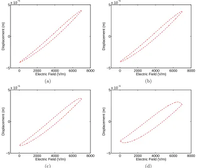
A crucial component in the AFM design for all of these applications is the piezoceramic (PZT)-based stage used to position the sample as depicted in Figure 1(a) [2, 4, 11, 13, 14]. Nested minor loops in data collected at 0.1 Hz are shown in Figure 1(b). Whereas PZT actuators provide the broadband and extremely high set point capabilities required by the AFM stages, they also exhibit frequency-dependent hysteresis as illustrated in Figure 2. At low frequencies, the hysteresis inherent to the these materials can be accommodated through PID or robust control designs [1, 9]. However, at the higher frequencies required by the previously outlined applications, increasing noise-to-data ratios and diminishing high-pass characteristics of control filters preclude a sole reliance on feedback laws to eliminate hysteresis. This motivates the development of control designs that incorporate and approximately compensate for hysteresis through model inverses employed either in feedback or feedforward loops.

0 2000 4000 6000 8000 −6

−4 −2 0 2 4

x 10−5

Electric Field (V/m)

Displacement (m)

(a) (b)

Figure 1: (a) PZT-based AFM stage. (b) Nested minor loops in data collected at 0.1 Hz on an AFM.

0 2000 4000 6000 8000 −5

0 5x 10

−5

Electric Field (V/m)

Displacement (m)

0 2000 4000 6000 8000 −5

0 5x 10

−5

Electric Field (V/m)

Displacement (m)

(a) (b)

0 2000 4000 6000 8000 −5

0 5x 10

−5

Electric Field (V/m)

Displacement (m)

0 2000 4000 6000 8000 −5

0 5x 10

−5

Electric Field (V/m)

Displacement (m)

(c) (d)

ψ

(P) = G(0,P)

P

P

P

P

G(E,P)

P

G(E,P)

P

P

E

E

P

E

P

P

E

E

P

E

P

Figure 3: Gibbs energyGand hysteronP resulting from the necessary condition ∂G_∂P = 0 for negligible thermal activation.

2. Constitutive Relations

To model the constitutive behavior of the piezoceramic stacked actuator, the stress-strain relation is assumed to be linear. However, the relation between the applied voltageV (or the applied fieldE) and the polarizationP

exhibits nonlinearities and hysteresis. The actuator is also assumed to be biased through poling so that the relation between P and the strain ε is linear for the considered operating conditions. To characterize the hysteretic E-P behavior at the domain level, a Helmholtz energy relation was derived in [15] using statistical mechanics principles under the assumption that dipoles are either aligned with the field or diametrically opposed to it. This model is appropriate for a single crystal with uniform effective fields. To construct a macroscopic model for a polycrystalline material with variable effective fields, the coercive and effective field values are then assumed to be distributed as detailed in the latter half of this section.

Under fixed temperature conditions with no applied stressσ, it is illustrated in [15] that a first order approx-imation to the statistical mechanics-based Helmholtz energy is the piecewise quadratic relation

ψ(P) =

       1

2η(P+PR)2 P ≤ −PI 1

2η(P−PR)2 P ≥PI 1

2η(PI−PR) ³

P2 PI −PR

´

|P|< PI.

(1)

As shown in Figure 3, PI is the positive inflection point andPR is the value of P at which the positive local

minimum ofψoccurs. The parameterηis the reciprocal of the slope of theE-P relation after switching occurs. This fact can be used to establish an initial parameter value forη when modeling a specific data set.

In the case of no applied stressesσ, the Gibbs energy can be formulated as

G(E, P) =ψ−EP (2)

where the second term represents the electrostatic energy due the applied fieldE. In order to include ferroelastic coupling, we utilize the extended Helmholtz relation

ψe(P, ε) =ψ(P) +

1 2Y

The Gibbs energy is then given by

G(E, P, ε) =ψ(P) +1 2Y

P_ε2_−YP_{γεP−EP −σε (4)}

whereσεincorporates the elastic energy. Note thatYP _{is the Young’s modulus for a constant polarization and}

γis a ferroelastic coupling coefficient.

In the case of negligible thermal activation, the local average polarization ¯P is determined from the necessary conditions

∂G ∂P = 0 ,

∂2G

∂P2 >0. (5)

Applying these conditions to (2) yields a piecewise linearE-P characterization

[ ¯P(E;Ec, ξ)](t) =     

[ ¯P(E;Ec, ξ)](0), τ(t) =∅ E

η −PR, τ(t)6=∅andE(maxτ(t)) =−Ec E

η +PR, τ(t)=6 ∅andE(maxτ(t)) =Ec

(6)

where

[ ¯P(E;Ec, ξ)](0) =      E

η −PR, E(0)≤ −Ec

ξ, −Ec < E(0)< Ec E

η +PR, E(0)≥Ec

(7)

and the transition times are

τ(t) ={t∈(0, Tf]|Et=−Ec or Et=Ec}. (8)

However, if thermal activation is significant, the dipoles can achieve the thermal energy required to switch in advance of the minimum Gibbs energy so the relative thermal and Gibbs energy must be balanced through Boltzmann principles. The probability density for achieving an energy levelGis then given by

µ(G) =Ce−GV /kT (9)

wherekis Boltzmann’s constant,V is a reference volume andCis a constant that is selected so that whenµ(G) is integrated over all possible dipole orientations, a probability of 1 is achieved. If we let 2σbe the separation between possible polarization states aroundP0, the probabilities of reaching a polarization state having sufficient

energy to switch orientations are given by

r+−= RP0+σ

P0−σ e

−G(E,P)V /kT_dP R_∞

P0−σe−G(

E,P)V /kT_dP , r−+= RP0+σ

P0−σ e

−G(E,P)V /kT_dP R_P0+σ

−∞ e−G(E,P)V /kTdP

. (10)

The likelihoods of reaching the required energy and thus of the dipoles switching from a positive to a negative orientation and conversely are then

p+− = 1

τr+− , p−+=

1

τr−+ (11)

where τ is the relaxation time. The fractions of dipoles in each orientation evolve according to the ordinary differential equations

dx+

dt =−p+−x++p−+x− , dx−

dt =−p−+x−+p+−x+. (12)

The expected polarizations due to positively and negatively oriented dipoles are

hP+i= Z _∞

P0+σ

P µ(G)dP , hP+i= Z _P0−σ

so the evaluation ofCyields

hP+i= R_∞

P0+σP e−G(E,P,T)V /kTdP R_∞

P0+σe−G(E,P,T)V /kTdP

, hP−i= RP0−σ

−∞ P e−G(E,P,T)V /kTdP RP0−σ

−∞ e−G(E,P,T)V /kTdP

. (14)

For a single crystal with uniform effective field, the local average polarization is subsequently

¯

P=x+hP+i+x−hP−i. (15)

In the manner detailed in [15], the evaluation of the integrals in (10) and (14) can be simplified through approx-imations employing the inflection points±PI rather than the unstable equilibriumP0.

Both of the relations (6) and (15) are valid only for homogeneous single crystal materials with uniform effective fields. To account for nonuniformity and inhomogeneities in the materials, local coercive and effective fields are assumed to be manifestations of underlying distributions rather than constants. The macroscopic polarization model is then given by

P(E) =

Z _∞

0 Z _∞

−∞

¯

P(E+Ee, Ec, ξ)ν1(Ec)ν2(Ee)dEedEc (16)

where ν1 and ν2 are appropriate densities. Motivated by choices in the magnetics literature, ν1 and ν2 were

respectively designated to be lognormal and normal densities in [15]. However, the fact that neither of these choices is based on energy considerations, motivates the consideration of general densities.

Based on physical arguments, we may assume that the general densities decay to zero. Therefore, the double integral can be evaluated by truncating the domains and using composite Gaussian quadrature. In this case, discretization of (16) gives

P(E) =

Ni X

i=1 Nj X

j=1

¯

P(E+Eej, Eci, ξi)ν1(Eej)ν2(Eci)viwj (17)

whereEej, Eci are the abscissas and vi, wj are the weights. Here, ν1(Eej) and ν2(Eci) are parameter values to

be determined. Details regarding the identification ofν1 andν2 can be found in [10].

Finally, the equilibrium condition

∂G

∂ε = 0 (18)

yields the elastic constitutive relation

σ=YPε−YPγP. (19)

This relation along with the nonlinear polarization relation (16) quantifies the constitutive behavior for the piezoceramic materials employed in the AFM.

3. Model Inverse

To construct a model inverse to be employed as filter in the robust control design, consider first an imple-mentation of the forward model (17) described in [15] and summarized below. Formulate the local polarization (6) as

P =E

η +PR∆ (20)

where ∆ is anNi×Nj matrix whose elements are either 1 or−1. Theijth entry in ∆ indicates whether thejth

effective field valueEej has crossed theith coercive field valueEci and thus whether the associated polarization

value is on the upper or lower branch of the hysteron. Now rewrite ∆ as a vector ∆vec with the order of the

entries determined by order in which the entries in ∆ change as the fieldE is increased or decreased. Thus ∆vec

A model for quantifying the inverse map betweenP andE is now outlined in Algorithm 1.

Algorithm 1.

SpecifyEprev,Pprev,Pnew

Ptemp=Pprev

while Ptemp< Pprev

Etemp = value ofE at which the next entry in ∆vec changes

Update next entry in ∆vec

Compute change inP and update P

Update Ptemp

end

ComputeEnew

4. Stacked Actuator Model

In addition to hysteresis, the dynamics of the actuator must be incorporated. We assume that the rod has cross-sectional area A, length `, density ρ and Young’s modulus YP_{. Let c}P _{be the Kelvin-Voight damping}

parameter andγ be the piezoelectric coupling coefficient. In the present stage design, depicted in Figure 1(a), one end of the actuator is fixed, while the attachment at the other end can be modeled as a damped spring-mass system. For this end, letMLbe the mass,kLbe the stiffness, andcLbe the damping coefficient. Force balancing

along the actuator then yields the relation

ρA∂

2_u

∂t2 = ∂N

∂x (21)

where the resultantN =R_AσdAis given by

N =YPA∂u

∂x +c

P_A ∂2u

∂x∂t −Y

P_{AγP(E). (22)}

Note thatudenotes displacement in the longitudinalx-direction and that the relation strain ε= ∂u_∂x is used in obtaining (22). The boundary conditions areu(t,0) = 0 at the fixed end and

N(t, `) =−kLu(t, `)−cL∂u

∂t(t, `)−ML ∂2u

∂t2(t, `) (23)

at the moving end. Initial conditions are given byu(0, x) = ∂u_∂t = 0. The polarizationP(E) is specified by (16). An approximate solution to (21) is found by first deriving a weak form

Z _`

0 ρA

∂2u ∂t2ψdx+

Z _`

0 ·

YPA∂u ∂x+c

P_A ∂2u

∂x∂t

¸

∂ψ

∂xdx=−

Z _`

0 Y

P_AβP(E)∂ψ

∂xdx (24)

and then discretizing in space with linear finite elements and in time with finite difference techniques. Details of the derivation of the weak form and the construction of the finite element and finite difference equations can be found in [13].

0 2000 4000 6000 8000 −6

−4 −2 0 2 4

x 10−5

Electric Field (V/m)

Displacement (m)

Data Model

0 2000 4000 6000 8000

−6 −4 −2 0 2 4

x 10−5

Electric Field (V/m)

Displacement (m)

Data Model

(a) (b)

0 2000 4000 6000 8000

−6 −4 −2 0 2 4

x 10−5

Electric Field (V/m)

Displacement (m)

Data Model

0 2000 4000 6000 8000

−6 −4 −2 0 2 4

x 10−5

Electric Field (V/m)

Displacement (m)

Data Model

(c) (d)

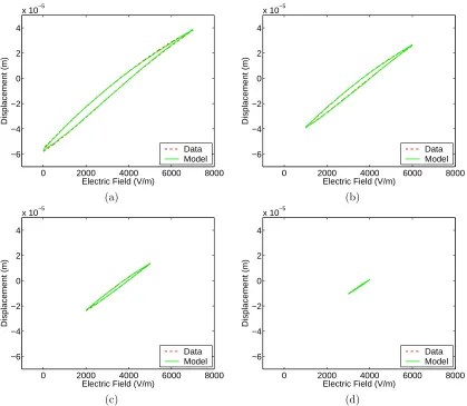
Figure 4: Characterization of AFM field-displacement behavior at 0.1 Hz.

5. Model Validation

To demonstrate the accuracy and efficiency of the hysteresis model, we consider the characterization of nested minor loops collected at 0.1 Hz as well asE-P behavior at frequencies ranging from 0.28 Hz to 27.9 Hz. In both cases, displacements were computed using the ODE model constructed using the stress relation (19) and hysteresis model (16) with general densitiesν1 andν2 identified using the techniques detailed in [10, 12].

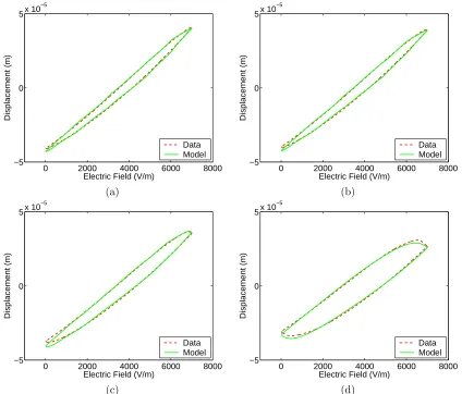
Figure 4 illustrates the capability of the model to characterize nested, biased minor loop behavior and Figure 5 demonstrates the characterization of frequency-dependent dynamics. The latter involves the quantification of both thermal relaxation and inertial effects as illustrated by the change in sign of the slope ∂P_∂E following field reversal. Further details demonstrating properties of the model for characterizing hysteresis in various PZT compounds can be found in [10, 11, 12, 15].

6. Robust Control Design

0 2000 4000 6000 8000 −5

0 5x 10

−5

Electric Field (V/m)

Displacement (m)

Data Model

0 2000 4000 6000 8000

−5 0 5x 10

−5

Electric Field (V/m)

Displacement (m)

Data Model

(a) (b)

0 2000 4000 6000 8000

−5 0 5x 10

−5

Electric Field (V/m)

Displacement (m)

Data Model

0 2000 4000 6000 8000

−5 0 5x 10

−5

Electric Field (V/m)

Displacement (m)

Data Model

(c) (d)

Figure 5: Characterization of AFM field-displacement behavior with sample rates of (a) 0.279 Hz, (b) 1.12 Hz, (c) 5.58 Hz, and (d) 27.9 Hz.

utilize the model inverse. After a discussion of the system representation, numerical examples are given to demonstrate the performance of the control designs.

The control design is analogous to that described in [5, 6, 7]. The physical control system is the AFM and the control objective is to track a reference trajectoryrwhich represents the displacement of the actuator. The system representation in shown in Figure 6. The plantP represents the ODE model for the AFM rod. The sensor noise in the measurement ofyis separated into two components,s, taken to be 60 Hz noise to simulate electromagnetic disturbances, andn, taken to be high frequency noise which can be attributed to the sensing device or external disturbances. The disturbanced represents errors in the plant input caused by either unattenuated hysteresis and constitutive nonlinearities or by discretization errors from the inverse filter. The output signalebrepresents the weighted tracking error andbuis the weighted output of the controllerK. The weighting functionsWr,We,

Wu,Wd, Ws, andWn are selected to achieve the best performance from the controller. They are chosen based

on known information about the corresponding signals.

W

_r

_We

W

W

K

u

d

r

+

−

e

u

Wn

s

W

y

u+d

_P

n

s

d

u

e

Figure 6: System representation including input disturbance dand sensor noisesandnin the transducer.

as

e = Wr[r]−(P[Wd[d] +u] +Wn[n] +Ws[s]

= Wr[r]−P[Wd[d]]−Wn−Ws[s]−P[u] b

e = We[e] b

u = Wu[u].

The transfer function matrixGfrom the inputsr,d,n,sanduto the outputse,ebandubis then specified by



We0Wr −We0P Wd −W0eWn −W0eWs −WWeuP

Wr −P Wd −Wn −Ws −P 

_. (25)

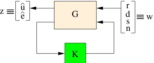
The linear fractional transformation system representation is shown in Figure 7 with details provided in [7, 17]. The choice of weighting functions is an important part of the control design. To filter the 60 Hz sensor noises, a sixth-order passband Chebyshev filter with a range of 55 Hz to 65 Hz is used forWs. The frequency response

ofWsis shown in Figure 8(a). The choice forWn is a second-order highpass Butterworth filter with a cutoff of

150 Hz which accommodates the high frequency sensor noisen. The weightWr is based on which components

of the reference signal are most important during tracking. For example, considering the 0.25 Hz sinusoidal part of the reference signal to be most important, a sixth-order passband Chebyshev filter with a range of 0.125 Hz to 0.375 Hz was employed. To determine the weighting filter Wd, the reference signal was scaled to have the

same order of magnitude as polarization. This signal was then fed into either the inverse filter or a linear filter to determine the scale from polarization and field. The result was then fed to the forward model. This process is depicted in Figure 9 for the two choices of disturbance. In both cases, the power spectrum of the outputd

had only low frequency components. Thus a second-order lowpass Butterworth filter with a cutoff of 10 Hz was used forWd. The frequency response ofWd in the case when the linear filter was used is shown in Figure 8(b).

The weighting function on the error signalewas chosen to be We=_s+γe_²e withγe= 1×101 and²e= 1×10−8.

An integrator was chosen so that the error would not achieve steady state at a nonzero value. Also, the pole was shifted slightly off zero to ensure that the controller was realizable. Finally, the weighting function on the controller output was chosen to beWu= 5×10−6.

r

s

d

n

w

z

_G

K

u

e

101 102 10−3

10−2 10−1 100

Frequency (Hz)

Magnitude

10−2 100 102 10−3

10−2 10−1 100

Frequency (Hz)

Magnitude

(a) (b)

Figure 8: (a) Frequency response of the passband filterWs(b) Frequency response ofWd for the disturbanced

due to scaled but uncompensated hysteresis and nonlinearities.

The transfer function matrix (25) gives a representation for the transducer system with weighting filters included. In order to formulate the control laws for computing the gains K, H2 and H_∞ norms of the closed loop system representationT are minimized. These are

kTk22=₂1_π Z _∞

−∞trace [T

∗_{(jω)T(jω)]dω , kTk}

∞= sup

ω∈lRσ¯[T(jω)] (26)

where σ[T(jω)] represent the maximal singular values of the closed loop map T. Details regarding this robust control formulation can be found in [7, 17].

7. Numerical Examples

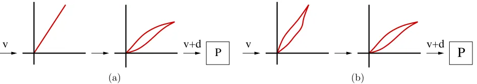
We consider the two possibilities for the disturbance depicted in Figure 9. The first, which is due to scaled but uncompensated hysteresis, yields the tracking results and errors shown in Figure 10. In the second case, the disturbance is due to errors existing in the inverse compensation procedure used to approximately linearize the transducer response. The tracking capabilities and errors for this case are shown in Figure 11.

A comparison between Figures 10 and 11 illustrates that highly accurate tracking is obtained in both cases, with errors less than 2µm maintained after the commencement of the periodic cycle. The equivalence in accuracy for the uncompensated and compensated designs is attributed to the low level of hysteresis present in this low frequency 0.25 Hz drive regime as demonstrated by the data in Figure 2. The present investigation focuses on the extension of these control designs to higher frequencies where increasing hysteresis levels necessitate inverse compensation as demonstrated for analogous magnetic model based controllers in [7].

Very similar results are obtained using theH_∞design, indicating that for this application, the construction of models and control filters may play a more important role than the choice of robust control laws for high accuracy tracking.

v+d

v

P

v

v+d

P

(a) (b)

0 5 10 15 20 0

5 10 15x 10

−5

Time

Position (m)

Reference Simulated

0 5 10 15 20

−6 −4 −2 0 2 4 6x 10

−6

Time

Error

(a) (b)

Figure 10: H₂ design with sensor noise s and the disturbance d due to inversion error. (a) Reference and simulated trajectory, and (b) tracking error.

0 5 10 15 20

0 5 10 15x 10

−5

Time

Position (m)

Reference Simulated

0 5 10 15 20

−6 −4 −2 0 2 4 6x 10

−6

Time

Error

(a) (b)

Figure 11: H₂design with sensor noisesand the disturbanceddue to uncompensated hysteresis and constitutive nonlinearities. (a) Reference and simulated trajectory, and (b) tracking error.

8. Concluding Remarks

We have summarized here the construction of macroscopic constitutive relations and models to characterize the hysteretic drive dynamics of a PZT-based AFM stage. These models extend previous formulations through the use of general density representations which provide high accuracy while maintaining implementational efficiency. The modeling framework also facilitates inversion for linear control design. The performance of initial robust control designs for high accuracy AFM drive regimes is illustrated through numerical examples.

9. Acknowledgements

References

[1] D. Croft, G. Shed and S. Devasia, “Creep, hysteresis, and vibration compensation for piezoactuators: Atomic force microscopy application,”Journal of Dynamic Systems, Measurement, and Control, 23, pp. 35-43, 2001. [2] A. Daniele, S. Salapaka, M.V. Salapaka and M. Dahleh, “Piezoelectric scanners for atomic force microscopes: Design of lateral sensors, identification and control,” Proceedings of the America Control Conference, San Diego, CA, pp. 253–257, 1999.

[3] DARPA Program on Molecular Observation, Spectroscopy and Imaging Using Cantilevers (MOSAIC), http://www.darpa.mil/dso/thrust/biosci/mosaic.htm.

[4] P.K. Hansma, V.B. Elings, O. Marti and C.E. Bracker, “Scanning tunneling microscopy and atomic force microscopy: Application to biology and technology,”Science, 242, pp. 209-242, 1988.

[5] J.M. Nealis and R.C. Smith, “H∞ Control Design for a Magnetostrictive Transducer,” Proc. 42nd IEEE Conf. Dec. and Control, Maui, HA, pp. 1801-1806, 2003.

[6] J.M. Nealis and R.C. Smith, “Robust Control of a Magnetostrictive Actuator,” Proceedings of the SPIE, Smart Structures and Materials 2003, Volume 5049, pp. 221-232, 2003.

[7] J. Nealis and R.C. Smith “Model-based robust control design for magnetostrictive transducers operating in hysteretic and nonlinear regimes,” CRSC Technical Report CRSC-TR03-25; IEEE Transactions on Auto-matic Control, submitted.

[8] D. Rugar, O. Z¨uger, S.T. Hoen, C.S. Yannoni, H.-M. Vieth and R.D. Kendrick, “Force detection of nuclear magnetic resonance,”Science, 264, pp. 1560-1563, 1994.

[9] S. Salapaka, A. Sebastian, J.P. Cleveland and M.V. Salapaka, “High bandwidth nano-positioner: A robust control approach,”Review of Scientific Instruments, 73(9), pp. 3232-3241, 2002.

[10] R.C. Smith and A. Hatch, “Parameter estimation techniques for nonlinear hysteresis models,” Proceedings of the SPIE, Smart Structures and Materials, to appear.

[11] R.C. Smith, A. Hatch and T. De, “Model Development for Piezoceramic Nanopositioners,” Proc. 42nd IEEE Conf. Dec. and Control, Maui, HA, pp. 2638-2643, 2003.

[12] R.C. Smith, A. Hatch, B. Mukherjee and S. Liu, “A homogenized energy model for hysteresis in ferroelectric materials: General density formulation,” preprint.

[13] R.C. Smith and M. Salapaka, “Model development for the positioning mechanisms in an atomic force microscope,”International Series of Numerical Mathematics, Vol 143, pp. 249-269, 2002.

[14] R.C. Smith, M.V. Salapaka, A. Hatch, J. Smith and T. De, “Model development and inverse compensator design for high speed nanopositioning,” Proceedings of the 41st IEEE Conference on Decision and Control, 2002, Las Vegas, NV.

[15] R.C. Smith, S. Seelecke, Z. Ounaies and J. Smith, “A free energy model for hysteresis in ferroelectric materials,”Journal of Intelligent Material Systems and Structures, 14(11), pp. 719–739, 2003.

[16] S.A. Wolf, D.D. Awschalom, R.A. Buhrman, J.M. Daughton, S. von Moln´ar, M.L. Chtchelkanova and D.M. Teger, “Spintronics: A spin-based electronics vision for the future,”Science, 294, pp. 1488-1495, 2001. [17] K. Zhou and J.C. Doyle,Essentials of Robust Control, Prentice Hall, New Jersey, 1998.

Note: Center for Research in Scientific Computation Technical Reports can be accessed at the web site